Article

Elevation Angle Characterization for LEO Satellites: First and Second Order Statistics

by
Juan Misael Gongora-Torres
*,†,
Cesar Vargas-Rosales
,
Alejandro Aragón-Zavala
and
Rafaela Villalpando-Hernandez
Tecnologico de Monterrey, School of Engineering and Science, Monterrey 64849, Mexico
*
Author to whom correspondence should be addressed.
These authors contributed equally to this work.
Submission received: 26 February 2023 / Revised: 18 March 2023 / Accepted: 21 March 2023 / Published: 30 March 2023
(This article belongs to the Special Issue Small Satellites Missions and Applications)

Abstract

:
The elevation angle θ is relevant for the Low Earth orbit (LEO) satellite communications since it is always changing its relative position with respect to fixed Earth stations (ES’s), and this affects the link length and received power, P R . This article provides a new methodology to compute the probability density function (PDF) and cumulative distribution function (CDF) of the elevation angle, θ , for diverse ES locations. This methodology requires as input parameters an ES latitude, ϕ , an orbit inclination value, i, and an orbit altitude, h. The elevation angle is characterized through a well known random variable, which facilitates the computation of the first and second-order statistics, and helps to determine the expected value and measures of dispersion of the angle θ for a particular ES location. The proposed methodology allows an easy and quick calculation of the elevation angle’s CDF, facilitating comparisons against CDF’s of more ES’s located at different latitudes, and longitudes, λ ; as well as the comparisons of CDF’s of the elevation angle produced by different orbits. Extensive simulation results are summarized in a small table, which allows computation of the elevation angle’s CDF and PDF for multiple ES locations without requiring of simulations and statistical fitting. Finally, the proposed methodology is validated through an extensive error analysis that show the suitability of the obtained results to characterize the elevation angle.

1. Introduction

The characterization of the elevation angle, θ is relevant for low Earth orbit (LEO) satellite communications since this parameter is directly related to the varying distance between the satellite and Earth station (ES), and affects the link total attenuation. The elevation angle description through an analytical expression is a difficult problem addressed in [1,2] which has received less attention in the literature.
Nonetheless, this parameter is directly related to the link performance and channel characterization of LEO satellites. The LEO channel characterization has also received less attention than the geostationary (GEO) satellite channel and just few models such as [3] have been specifically developed and published to consider the elevation angle variations introduced at LEO. The lack of LEO channel models accounting for the always-changing elevation angle have resulted in just a few channel models available in the literature for LEO satellites and specially for small satellites as mentioned in [4].
LEO satellites are increasing their numbers and role as an enabling technology for Internet of Things (IoT), 5G, 6G, and next generation wireless networks aimed to provide global coverage with very low latency [5]. Then it is relevant to develop methodologies to analyze and compare the link performance and channel characteristics considering the variations introduced by the always-changing elevation angle.
The always-changing elevation angle condition has been a limitation to analyze the link budget and channel of LEO satellites, and common approaches to characterize it have followed segmentation in best and worst-case of the elevation angle [6], instead of analyzing the short and long term behavior of the elevation angle as an analytical function. However, some emerging problems, such as efficient power management [7], related to LEO satellites have made evident the necessity of having a way to characterize the elevation angle as an analytical function.
The observed elevation angle, θ , is always-varying for LEO satellites and can be described as a function of time, θ ( t ) , for intervals in which a satellite is visible. The calculation of θ for a given position can be deterministically obtained with mathematical procedures developed in orbital mechanics books [8] and widely implemented in software for space dynamics simulations. However, it is important to note that even with accurate predictions of θ (accounting for contacts in several days or months), the relations between one contact and another, as well as the long term behavior of the elevation angle can be hardly described without randomness. Thus, appropriate use of probability theory becomes a great tool to analyze the behavior of the elevation angle, θ , in the long term.
The elevation angle, θ , is usually defined for an ES as the angle (above the local horizon) at which the satellite is visible, and within the interval of 0° to 90°, θ ( 0 ° , 90 ° ] , regardless of its azimuth. The minimum value of θ at which communication is possible is often called θ m i n (subject to θ m i n 0 ° ), similarly, the maximum value of θ that can be observed from the ES is called θ m a x (subject to θ m i n θ m a x 90 ° ). We can define a random variable, r.v., to take possible values of θ , such that θ ( θ m i n , θ m a x ] as Θ .
The probability density function, PDF, and cumulative distribution function, CDF, of the elevation angle, f Θ ( θ ) and F Θ ( θ ) , respectively, are useful functions to characterize the LEO channel since the elevation angle affects the received power level, P R . The reasoning behind that is that θ depends on the distance from the satellite to the ES, r S , E . Then, at greater link distances, it can be expected to have a lower received power, P R , (of the transmitted signal from the satellite) than at shorter distances.
The distance between a LEO satellite and an ES, r S , E , can vary several thousands of kilometers from a low value of θ to a high value of θ . Figure 1a shows the extreme cases for the elevation angle in a LEO satellite link. Those extreme cases are not necessarily met at every contact, but represent the best and worst length-scenarios in a long period. Path lengths between the ES and satellite, r S , E , are described in this figure using the variable r i , i { 1 , 2 , 3 } . The figure also shows that at low values of θ the path length is larger and the received power, P R is at its minimum value. This last implication between the elevation angle, θ , the received power, P R , and the link length, r S , E , assumes some constraints explained in detail in [9].
Figure 1b shows the typical-case for the elevation angle, where the value of θ is not necessarily at its minimum nor at its maximum, but it can be at any value within the range θ [ θ m i n , θ m a x ] . Since the elevation angle of a LEO satellite appears as always-varying from an ES’s, it is convenient to determine statistical indicators of its behavior, such as its expected value, E [ · ] , median, M E D [ · ] , standard deviation, S D [ · ] ; and how often does the elevation angle will be above or below a threshold, or within a region of interest, for example, using its quantiles n Q . In addition, since the elevation angle variations are directly related to the link length, the elevation angle for LEO satellites is also directly related to the variations of the received power P R at an ES, as described in [9].

1.1. Contributions

The elevation angle characterization is relevant for LEO satellites because it is an always-changing variable for those communication systems. The effects of the elevation angle variations are observable in the received power, link quality, and channel behavior; then, an accurate characterization of this variable is a topic of interest for planning and implementation of LEO satellite systems.
In this article, we have addressed the characterization of the elevation angle for LEO satellites, by obtaining its PDF and CDF, as well as the derivation of its first and second order statistics. First and second order statistics are relevant to evaluate the suitability of different LEO orbits and to determine which orbits are more convenient to provide coverage for a particular application or Earth station location.
In addition, we have developed an extensive analysis to validate our results, and we include supplementary materials containing elevation angle times series. The supplementary materials will facilitate reproducibility of our work, and will allow future research based on our proposed methodology and results.

1.1.1. Contribution 1

This document shows the feasibility of using a random variable to characterize the elevation angle behavior for LEO satellites with different orbit configurations. The suitability of using the proposed random variable is verified through an extensive error analysis with diverse orbit configurations.

1.1.2. Contribution 2

The PDF and CDF of the elevation angle can be obtained as proposed in [1,2]. Nonetheless, this document describes a methodology to obtain the PDF and CDF parameters of the elevation angle distribution for different orbit configurations and ES locations using a well-known random variable. The proposed random variable facilitates analytical manipulation as well as computation of the probabilities of occurrence of the elevation angle at specific values. A small table containing the resultant parameters to characterize multiple LEO orbits configurations as observed from multiple ES’s is included.

1.1.3. Contribution 3
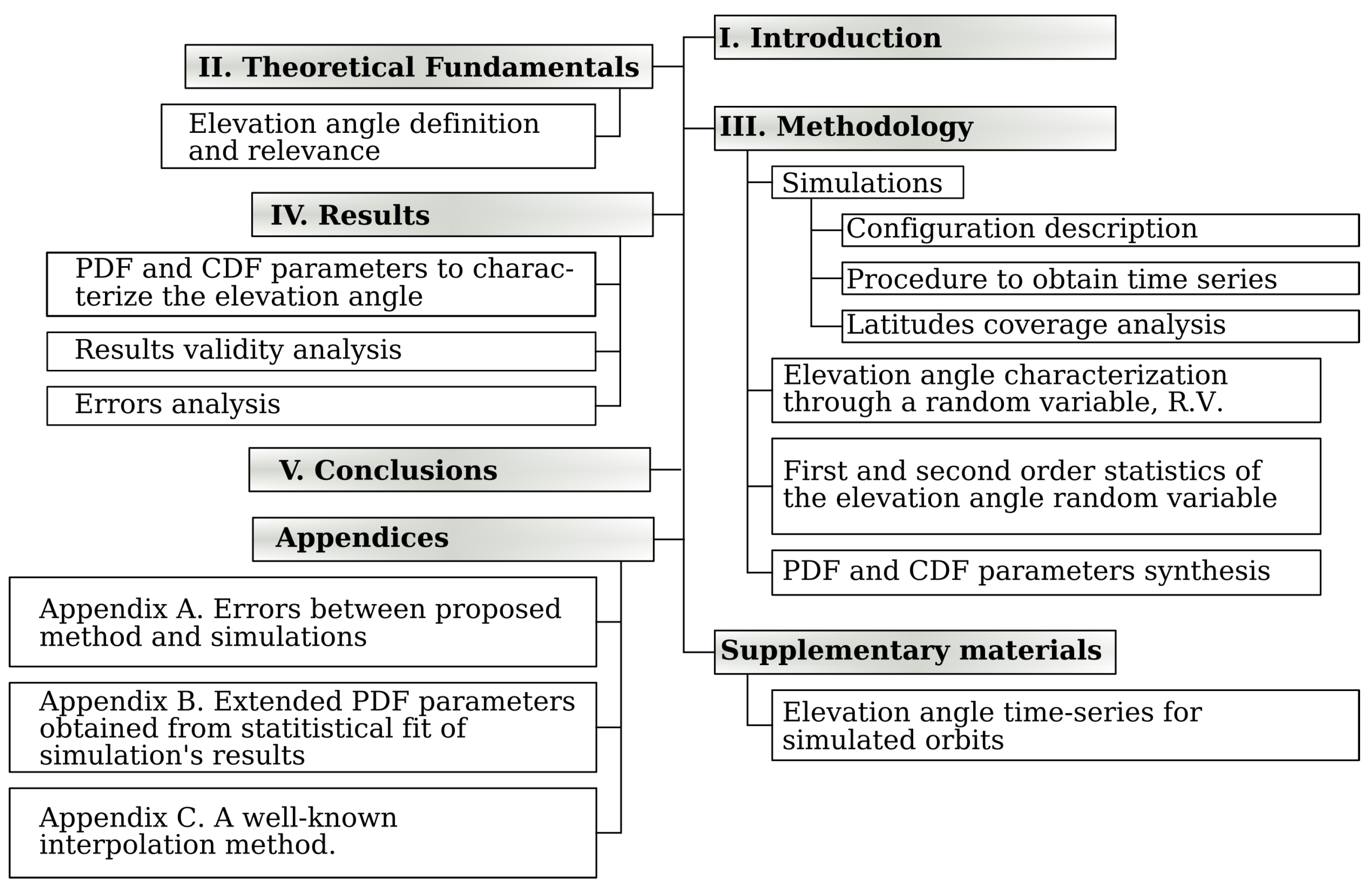
The expected value of the elevation angle and its measures of dispersion are relevant for planning and implementation of LEO satellite systems, since the received power varies according to the elevation angle. This document describes an analytical methodology to obtain the first and second order statistics of the elevation angle for different orbit configurations and ES locations, which, to the best of our knowledge are not available in the literature and were just utilized for a specific case in [9].

1.2. Outline

The remaining of the article is organized as follows: Section 2 introduces the theoretical fundamentals required to understand the subsequent sections; Section 3 describes the developed methodology to characterize the elevation angle behavior through f Θ ( θ ) and F Θ ( θ ) ; Section 4 contains the main results; and Section 5 concludes analyzing the obtained results and opportunities for future work. Figure 2 shows the main structure of the document.

2. Materials and Methods

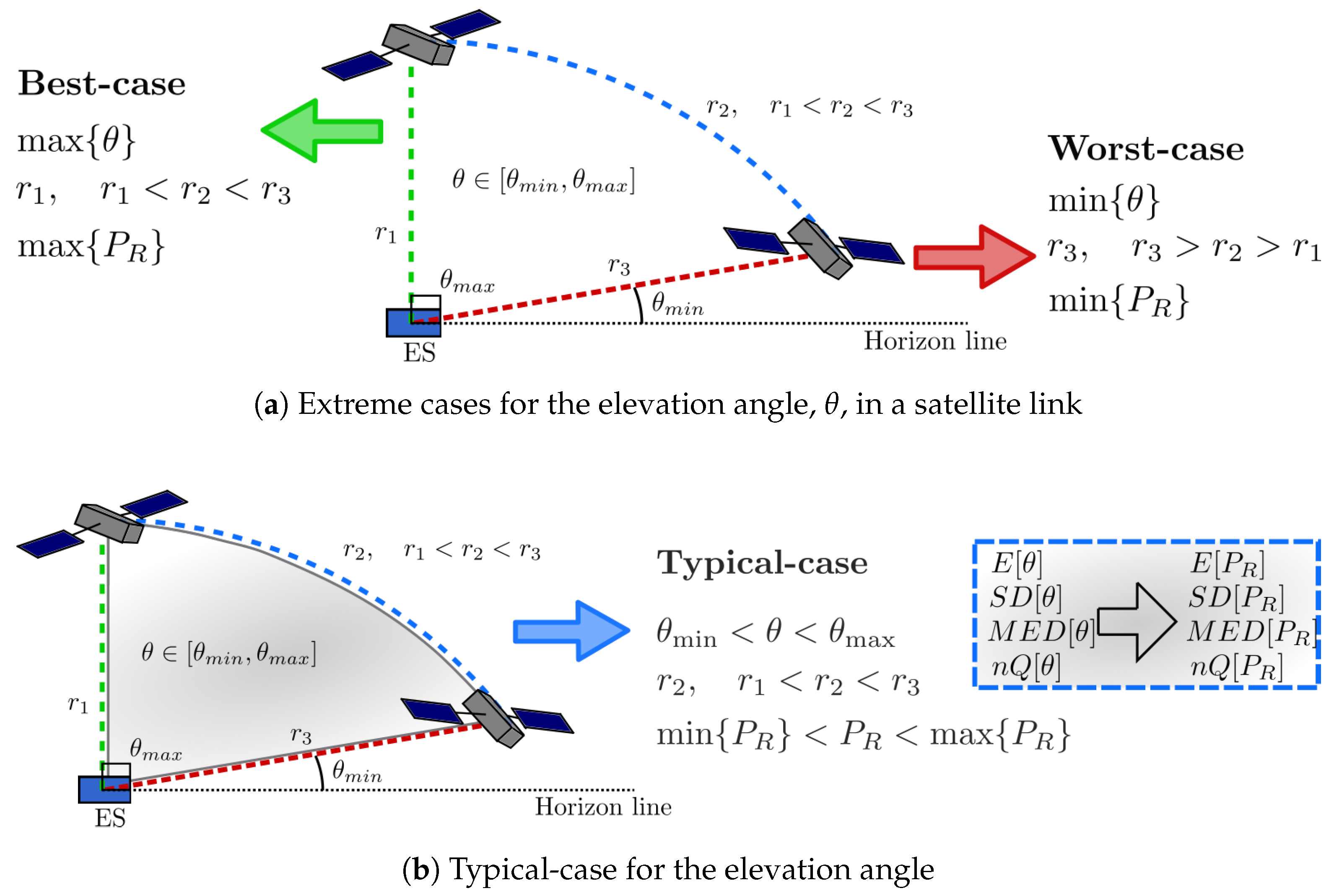
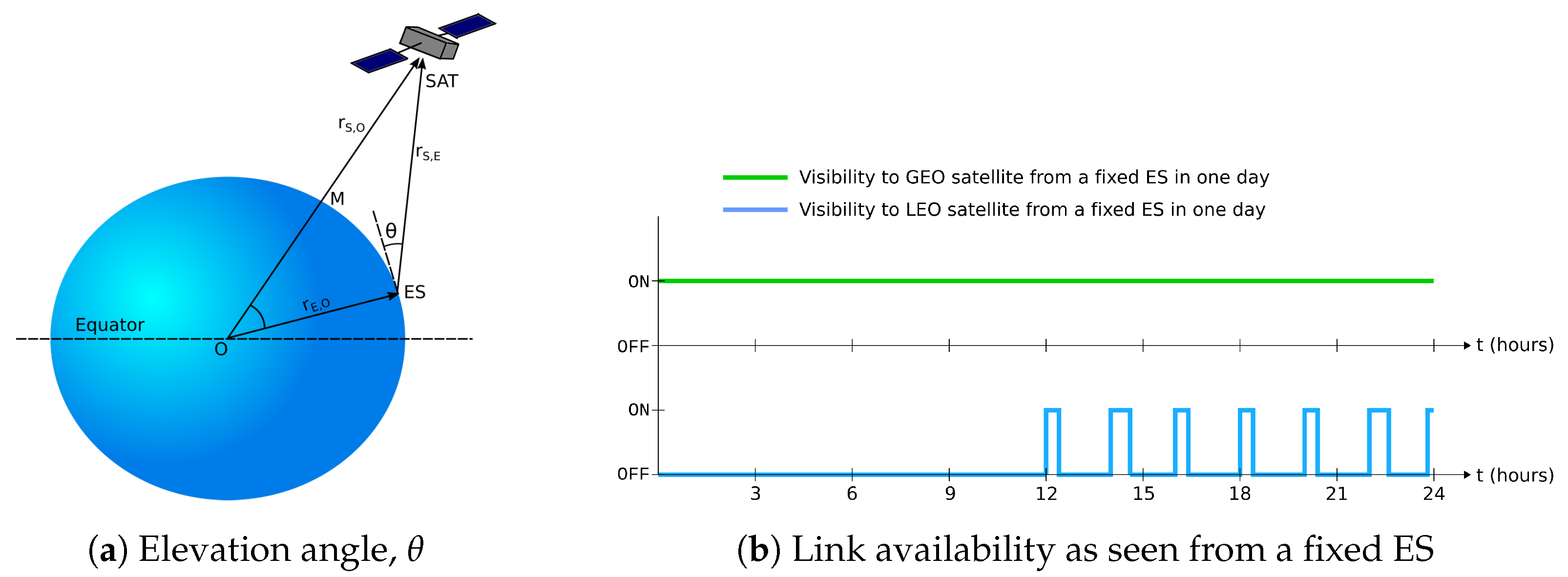
2.1. Elevation Angle Definition

The elevation angle, θ , for an ES can be defined as the angle between the local horizon and the satellite. Several sources such as [10,11,12] contain expressions to calculate θ from geometrical relations between the satellite and the ES instantaneous positions. One of those definitions is as follows
θ = arctan cos Δ cos ϕ ES ( r E , O / r S , O ) 1 cos 2 Δ cos 2 ϕ ES ,
where r E , O and r S , O are the distances from the center of the Earth, O, to the ES and the satellite, respectively; ϕ ES is the latitude at which the ES is located (in degrees); M is the subsatellite point, which corresponds to the latitude and longitude of the satellite instantaneous position; and Δ is the difference in longitude between the ES and M (in degrees). Figure 3a shows a derivation of θ based on (1).

2.2. Relevance of the Elevation Angle for the Satellite Channel

LEO satellites differ to those at GEO in its relative position as seen from a fixed ES. Whereas GEO satellites appear as fixed, those at LEO appear as always-moving points in the sky or are absent causing link unavailability. Link availability can be seen as an ON-OFF process, where the link is ON if the satellite is visible in the sky, and it is OFF if the satellite is absent. Figure 3b shows the ON-OFF process for both a LEO and GEO satellite.
In addition to the short visibility that LEO satellites have, conditions in this lapse are always varying as a consequence of the changing position of the satellite. When the satellite is first visible from an ES, it is at the largest distance supported by the link, then, the satellite starts approaching the ES until reaching the shortest distance in that particular contact. Finally, the satellite moves away after being at its minimum contact distance. It is important to note that the minimum distance from an ES to a LEO satellite, min ( r E , S ) , varies from one contact to another, as well as max ( r E , S ) does.
Differences between the Earth’s rotation rate and LEO orbiting velocities cause an always-varying link length (as seen from a fixed ES), and then, an always-varying elevation angle.
An important relation that needs to be accounted for the elevation angle, θ , and the link length, r S , E is given by the implication that when the angle is minimum, the  r S , E distance is maximum, i.e.,
θ min ( θ ) r S , E max ( r S , E ) ,
similarly
θ max ( θ ) r S , E min ( r S , E ) ;
where the maximum link length, max ( r S , E ) , occurs at some value of θ such that min ( θ ) < θ 90 ° ; and min ( r S , E ) occurs at some value of θ 0 ° lower than θ m a x . The implications in (2) indicate that when values of θ diminish, r S , E increases; similarly, in (3), when values of θ increase then r S , E decreases.
As a satellite moves away from an ES, r S , E and the free-space path loss, L F S , increases. Longer paths occur for lower values of θ , then, the atmospheric attenuation, A A t m , increases for larger paths (assuming similar atmospheric conditions for different link paths). On the other hand, when θ takes values close to 90 ° , r S , E will be at its minimum, and so does A A t m . Then, low elevation angles cause a greater L F S , and more atmospheric attenuation, A a t m (assuming that the atmospheric conditions are approximately the same for two distinct paths).
For LEO it is important to consider link interference, I, usually addressed as noise in link-budget calculations, and also dependent on the elevation angle as mentioned in [13]. Furthermore, low values of θ are also associated in practice with non-line-of-sight (NLOS) conditions, increasing ground interference [14], and increasing multipath fading in the land mobile satellite (LMS) channel [15,16,17].
There are several models available in the literature to characterize the received signal from satellite systems. Most of these works have been elaborated for the LMS channel, which describes the received signal at a land-moving ES; nonetheless, most of those works focus on GEO systems. Extensive reviews for the LMS channel can be found at [16,18,19].
Among the available channel models for LMS systems, a few of them focus on characterizations for LEO and non-GEO (NGEO) satellites; but, as noted by [4,20], those are few and there are still many challenges. Most of channels for NGEO systems have been developed based on previous models for GEO satellites, specially on well-known models, such as those by Loo [21] and Lutz [22].
Even though the Loo and Lutz models were not originally intended for LEO satellites, those were later used as a base for much of the non-geosynchronous (NGSO) channel models. The Loo channel assumes that the complex envelope of the received signal, r T , contains a LOS, r D , and a multipath component, r M , which in its phasor notation can be represented as
r T exp ( j ϕ T ) = r D exp ( j ϕ D ) + r M exp ( j ϕ M )
where ϕ T , ϕ D , and  ϕ M indicate the phase of the total received signal, of the direct or LOS component, and of the multipath component, respectively.
The channel developed by Lutz [22] models a varying received signal affected by different levels of shadowing. This channel is characterized by a Markov chain with a state corresponding to light shadowing, G, and another corresponding to deep shadowing conditions B. Figure 4 illustrates the Lutz channel.
The Loo channel [21] was adapted by Corazza and Vatalaro [3] to formulate one of the best-known channel models for LEO satellites; similarly, it was modified by Abdi et al. [23], to achieve straightforward analytical expressions for the first and second order statistics of the received signal based on the Nakagami distribution. However, current models for GEO and NGEO systems have recognized the limitations of a single distribution and a single state to describe the received signal, and mutistate models with different distributions at each state have became popular.
Channel models for LEO with multiple states as in [22] have been developed containing the same kind of distribution at each state. For example, a combination of the Lutz and Loo models was implemented for NGSO by Perez-Fontan et al. [24], focusing on time series generation. This model used a three-state Markov chain, as shown in Figure 5, to indicate different levels of shadowing; the first state, S 1 , indicates deep shadow; the second, S 2 , indicates moderate shadowing; and the third state, S 3 , indicates line-of-sight (LOS) conditions. Each state describes the received signal according to a Loo distribution with a different Loo triplet, α , ψ , M P ; and a different Markov chain for distinct elevation angle values. The so-called Loo triplet, which includes the mean of the direct signal amplitude, α , the standard deviation of the direct signal amplitude, ψ , and the multipath power, M P , is the set of parameters required by the Loo distribution.
Figure 6 shows two Loo distributions to characterize the satellite channel at two elevation angles; the CDF’s were computed assuming presence of a LOS component, and a multipath power component very close to the LOS level. The Loo distributions in Figure 6 can be understood as two of the states of Figure 5 at different elevation angles; e.g., a state transition from S 3 , θ 1 to S 3 , θ 2 .
In addition to the shadowing level at a receiver environment, which is mainly determined by natural and human made objects at the surroundings of the ES, the received signal level will be changing according to the elevation angle value. For LEO satellites, the elevation angle will change rapidly, and with a different rate at every contact.
As observed in Figure 6, the Loo CDF curves of the received signal rely on the elevation angle value since those depend on the LOS component of the received signal, α . Then, in order to predict different curves we need to know the expected value and measures of dispersion of the elevation angle.
Even though we illustrate the received signal through the well-known Loo model in Figure 6, there are more LEO channel models depending on a line-of-sight component, and thus, directly depending on the elevation angle. The, elevation angle characterization proposed in this article can be a valuable tool to determine CDF curves of the received signal, based on the first and second order order statistics of the elevation angle. For example, to determine the expected CDF of the Loo model based on the elevation angle expected value, and determine how far apart other curves will be based on the measures of dispersion of the elevation angle.

2.3. Analytical Characterization of the Elevation Angle

The elevation angle was analytically characterized in [2] through its probability density function (PDF), f Θ , which is defined as a marginal distribution from the joint PDF of Θ and the maximum value of the elevation angle, Θ m a x , as follows
f Θ ( θ ) = θ θ M f Θ , Θ m a x ( θ , θ m a x ) d θ m a x
where f Θ , Θ m a x is given by
f Θ , Θ m a x ( θ , θ m a x ) = f Θ | Θ m a x ( θ | θ m a x ) f Θ m a x ( θ m a x )
or equivalently
f Θ , Θ m a x ( θ , θ m a x ) = G ( θ ) sin γ ( θ ) cos 2 γ ( θ m a x ) cos 2 γ ( θ ) · f Θ m a x ( θ m a x ) θ m i n θ M f Θ m a x ( x ) cos 1 cos γ ( θ m i n ) cos γ ( x ) d x
The integral dividing the right hand term is a constant, say C 1 , then, (7) can be rewritten as
f Θ , Θ m a x ( θ , θ m a x ) = f Θ m a x ( θ m a x ) G ( θ ) sin γ ( θ ) C 1 cos 2 γ ( θ m a x ) cos 2 γ ( θ )
and the auxiliary functions γ ( · ) and G ( · ) require an extra parameter a defined as α = r E / r S , where r E = 6378 km is the radius of the Earth; and r S = r E + h depends on the altitude h (from the Earth’s surface) of the circular LEO orbit in kilometers. The functions γ ( · ) and G ( · ) are defined as follows
γ ( θ ) = cos 1 ( α cos θ ) θ
G ( θ ) = 1 + α 2 2 α cos γ ( θ ) 1 α cos γ ( θ )
The term f Θ m a x ( θ m a x ) is defined as follows
f Θ m a x ( θ m a x ) = G ( θ m a x ) K 2 · f Φ ( ϕ 0 γ ( θ m a x ) ) , for θ m i n θ m a x < θ c
f Θ m a x ( θ m a x ) = G ( θ m a x ) K 2 · [ f Φ ( ϕ 0 γ ( θ m a x ) + f Φ ( ϕ 0 + γ ( θ m a x ) ) ] , for θ c < θ m a x < θ M
where f Φ ( ϕ ) is defined from the orbital inclination i; and ES latitude, ϕ , as follows
f Φ ( ϕ ) = cos ϕ π sin 2 i sin 2 ϕ , for | ϕ | < i
and θ M = π / 2 , and  K 2 is given by
K 2 = 1 2 1 π sin 1 sin ( ϕ + γ ( θ m i n ) ) sin ( i )
where θ m i n is the minimum elevation angle that will be considered and is in the range 0 ° < θ m i n < 90 ° .
Although results shown in [2] are highly accurate with respect to the actual elevation angle PDF, the analytical expression f Θ is cumbersome to obtain and evaluate. Furthermore, analytical expressions for second or higher order statistics, are a missing result in the literature to the best of our knowledge.

3. Methodology for the Elevation Angle Characterization

In this section, we describe the procedure to characterize the elevation angle behavior through a random variable in a manageable analytical expression. Also, we include a procedure to obtain useful expressions of the elevation angle, such as measures of central tendency and dispersion.
The elevation angle characterization for different LEO orbit’s configuration will help to predict which orbits are more convenient for a particular ES location. In addition, the measures of central tendency and dispersion will help to choose suitable orbits based on the expected elevation angle, and to calculate the link attenuation based on the distribution of the elevation angle, and on its expected value and variance.

3.1. Simulations Configuration

Simulations were performed for a LEO satellite with characteristics mentioned in Table 1, and for circular orbit configurations listed in Table 2. The LEO region goes from a few hundred kilometers above the Earth’s surface up to 2000 km; but the performed simulations and methodology cover just the upper part of this region since orbit perturbations effects are much lower at those altitudes than at orbital heights closer to the surface, and facilitates operation for longer periods of time without a complex propulsion system.
Three initial values of orbital parameters not included in Table 2 are right ascension of the ascending node, Ω , argument of perigee, ω , and true anomaly, ν , which were all set to zero. From those simulations, ephemeris files with the satellite position and velocity in five-second steps were generated. Then, ES’s were placed (simulated) at 18 different and arbitrarily chosen locations listed in Table 3. Finally, time series of the observed elevation angle from the ES to the satellite were calculated for each ground location using the previous generated ephemeris files and geometrical relations as in (1).
The orbital mechanical equations required to calculate the position and velocity of the satellite as a function of time, were solved using an open source program developed and maintained by the NASA, GMAT [25]. The time series for the elevation angle discussed in this paper can be generated in GMAT using the data of Table 1, Table 2 and Table 3; also, these can be generated using other software, for example STK as in [2]. The time series mentioned in this paper were generated by the authors specially for this work, and are available at [26].

3.2. Elevation Angle Time Series Analysis
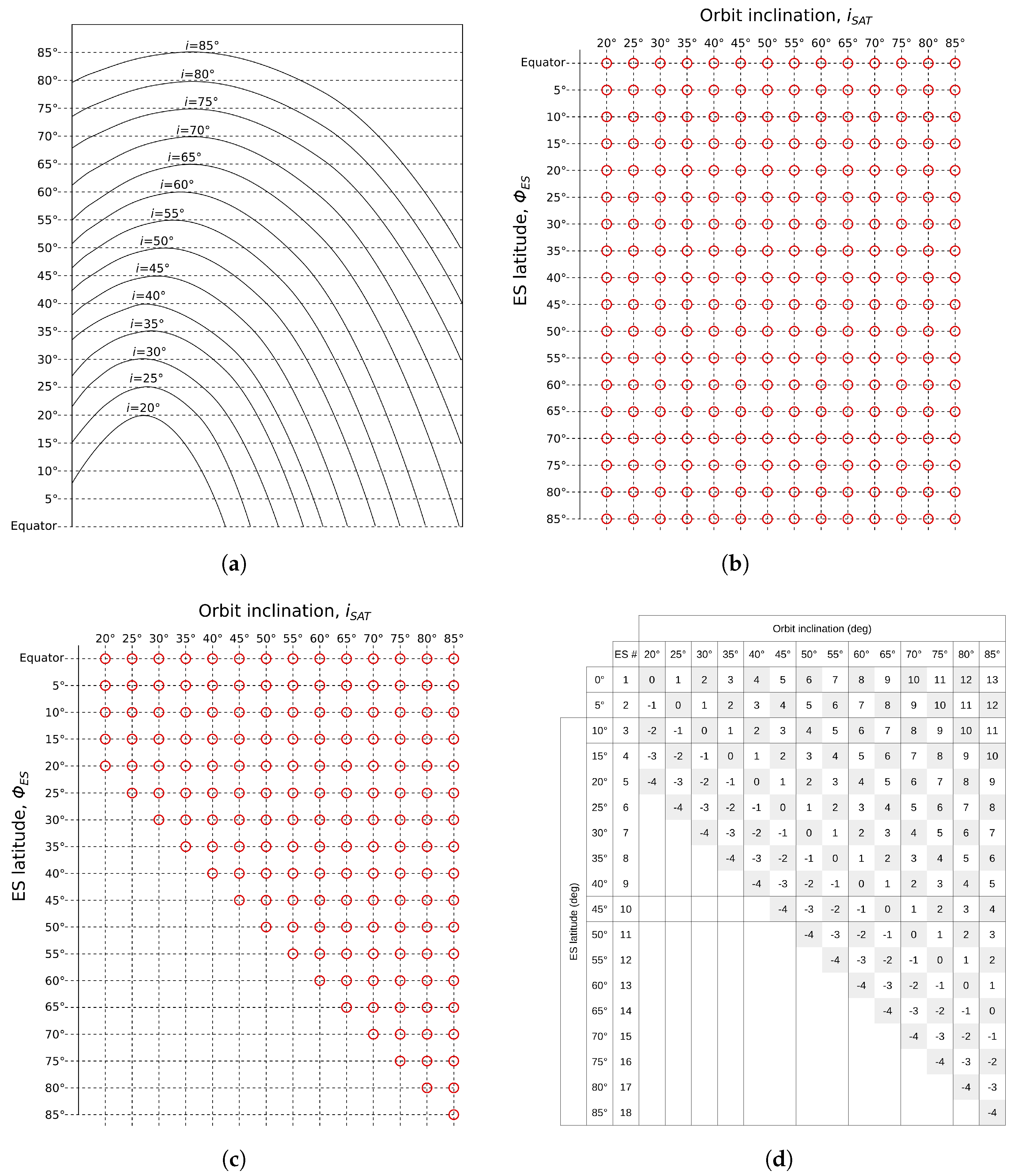
Each elevation angle data set (obtained from the simulations) was individually analyzed to observe its statistical values of interest (mean, median, standard deviation, quantiles). Those time series were fitted to several distributions using the maximum likelihood estimation method. The goodness of fit of the proposed distributions was evaluated for each elevation angle time series using the Kolmogorov-Smirnov test, and it was observed a better performance of the gamma distribution, G a m m a ( a , b ) , for most of the data sets. Other distributions that showed good fit based on the Kolmogorov-Smirnov test were the beta, B ( a , b ) , and Weibull, W e i b ( a , b ) . Figure 7 shows the values of θ as well as the PDF and CDF for one elevation angle time series, θ ( t ) using the proposed distributions. Figure 8 shows the Kolmogorov-Smirnov statistic, often indicated as D, for the time series obtained for different altitudes. The Kolmogorov-Smirnov statistic is an indicator of the maximum distance between the actual time series distribution and the proposed gamma distribution. A low value of the Kolmogorov-Smirnov is often desirable to indicate a better goodness-of-fit.
The gamma PDF, f Θ ( θ ) , and CDF, F Θ ( θ ) , are defined as follows
f Θ ( θ ) = 1 b a Γ ( a ) θ a 1 exp ( θ / b ) ,
and
F Θ ( θ ) = 1 Γ ( a ) γ a , θ b ,
respectively, where Γ ( · ) is the gamma function, γ ( · ) is the incomplete gamma function, a is the shape parameter, and b is the scale parameter. By definition both a and b are greater than zero.
The shape, a, and scale, b, parameters for the gamma distribution were obtained for each of the elevation angle time series of each ES. Those parameters were organized into several matrix arrays as shown in Table 4, which contains the shape parameter for the simulated orbits as seen from the ES 1 , and as in Table 5, which contains the scale parameter also for ES 1 .

3.3. Orbit Coverage

Figure 9a illustrates (without scale) passes of a satellite in each one of the six altitudes and for all the inclinations mentioned in Table 2. This figure also shows dashed lines indicating the ES’s latitudes mentioned in Table 3.
In Figure 9a as in Table 2 the orbit inclination parameter, i, for each altitude goes from 20 ° to 85 ° , then, this figure can be redrawn as the grid shown in Figure 9b, where the curved lines of Figure 9a are replaced by vertical lines indicating the orbit inclination. Additionally, the ES latitude lines were inverted to start with the lowest value at the top.
From Figure 9a it can be observed that satellites with certain orbit inclination i, reach (in its orbit trajectory) at most the latitude that coincide with the inclination value. For example, a satellite with i = 20 ° will not be able to pass over and ES located at ϕ = 80 ° , since the maximum reached latitude in that orbit will be ϕ i 20 ° , then, that satellite will be best suited to provide coverage at ES’s located at latitudes ϕ i or at most ϕ i . This coincides with basic knowledge of satellite coverage; whereas polar orbits can cover almost all the globe, lower inclination orbits cover smaller portions of the Earth. Then, we can redraw Figure 9b to have a coverage grid by discarding points corresponding to cases of ϕ E S > i S A T , this resultant grid is shown in Figure 9c.
From the simulation results obtained for the grid points of Figure 9c, matrices A h and B h containing the shape and scale parameters of f Θ ( θ ) and F Θ ( θ ) can be defined as follows
A h = a 1 , 1 a 1 , 2 a 1 , 3 a 1 , 14 a 2 , 1 a 2 , 2 a 2 , 3 a 2 , 14 a 3 , 1 a 3 , 2 a 3 , 3 a 4 , 1 a 4 , 2 a 4 , 3 a 5 , 1 a 5 , 2 a 5 , 3 N a N a 6 , 2 a 6 , 3 N a N N a N a 7 , 3 N a N N a N N a N a 18 , 14 18 × 14 , B h = b 1 , 1 b 1 , 2 b 1 , 3 b 1 , 14 b 2 , 1 b 2 , 2 b 2 , 3 b 2 , 14 b 3 , 1 b 3 , 2 b 3 , 3 b 4 , 1 b 4 , 2 b 4 , 3 b 5 , 1 b 5 , 2 b 5 , 3 N a N b 6 , 2 b 6 , 3 N a N N a N b 7 , 3 N a N N a N N a N b 18 , 14 18 × 14 ,
where N a N ’s are placed for the case ϕ E S > i S A T , and  h h s corresponds to the simulation altitudes set defined in Table 2 as
h s = { 1000 km , 1200 km , , 2000 km } .
Table A1, Table A2, Table A3, Table A4, Table A5 and Table A6 in Appendix B, show the shape and scale parameters obtained from simulations with configurations shown in Table 1, Table 2 and Table 3. From those values, matrices A h and B h can be constructed, and linear interpolation can be applied to those in order to obtain shape and scale parameters for different orbit inclinations, ES’s latitudes, and altitudes that were not simulated, but are in the range of h s , i s , ϕ s .

3.4. Reducing the Shape and Rate Matrices

From the grid of Figure 9c, an array as shown in Figure 9d can be created for each simulated orbit altitude. Figure 9d shows the diagonal numbers of a rectangular matrix D h defined as
D h = d 0 d 1 d 2 d 13 d 1 d 0 d 1 d 12 d 2 d 1 d 0 d 3 d 2 d 1 d 4 d 3 d 2 N a N d 4 d 3 N a N N a N d 4 N a N N a N N a N d 4 18 × 14 ,
for each altitude h h s , with  N a N ’s are placed for cases where ϕ E S > i S A T .

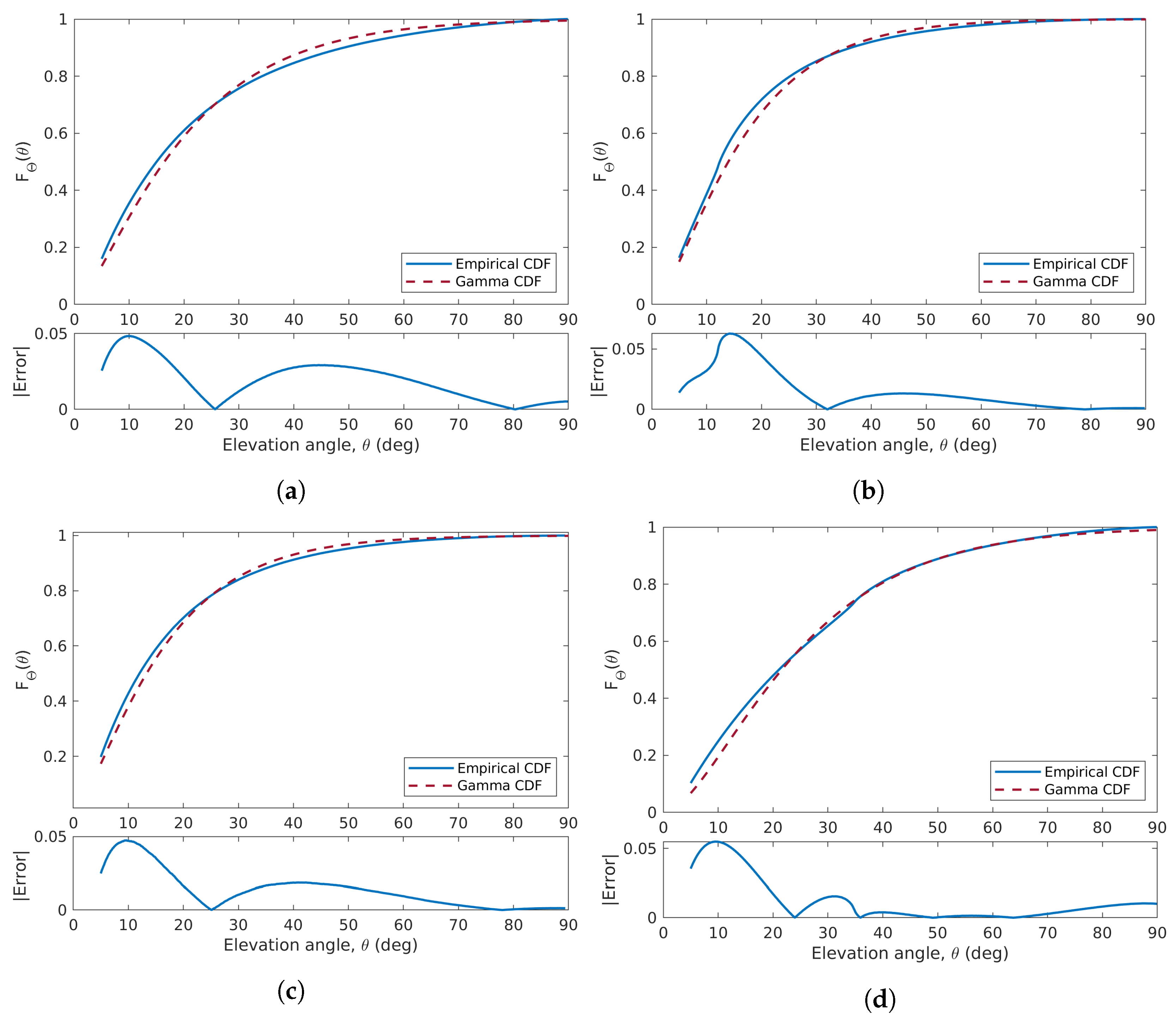
3.5. PDF and CDF of the Elevation Angle

In addition to h s , we can define two additional sets containing the orbit inclinations (as in Table 2) and ES’s latitudes (as in Table 3) at which simulations were performed, as 
i s = { 20 ° , 25 ° , , 85 ° }
and
ϕ s = { 0 ° , 5 ° , , 85 ° } ,
respectively.
Depending on the input values of ϕ k , h k , and  i k , if those are part of the previously defined sets ( i s , h s , ϕ s ) eight cases can arise as follows:
  • Case 1. i k i s and ϕ k ϕ s and h k h s
  • Case 2. i k i s and ϕ k ϕ s and h k h s
  • Case 3. i k i s and ϕ k ϕ s and h k h s
  • Case 4. i k i s and ϕ k ϕ s and h k h s
  • Case 5. i k i s and ϕ k ϕ s and h k h s
  • Case 6. i k i s and ϕ k ϕ s and h k h s
  • Case 7. i k i s and ϕ k ϕ s and h k h s
  • Case 8. i k i s and ϕ k ϕ s and h k h s
Case 1 occurs when all the input values ϕ k , i k and h k are contained in ϕ s , i s , and  h s , respectively; and Case 8 occurs when none of ϕ k , i k and h k parameters coincide with previously simulated values. Cases 2 to 7 occur when at least one of the input values (any of ϕ k , i k , and  h k ) coincides with a value within its corresponding sets ϕ s , i s and h s . Those cases illustrate all possible scenarios, ranging from not-required interpolation to interpolation inside a four-point mesh.
We can represent the ES latitude, ϕ k , orbit inclination, i k , or both (for which we want to determine their PDF) as a query point between two-known points, inside a three-point mesh, or inside a four-point mesh. Then we can use an interpolation method, such as those proposed in Appendix C, to find an appropriate value for the gamma distribution parameters at that query coordinates. In addition to those proposed in Appendix C, more interpolation methods are widely available in the literature.

3.6. First and Second Order Statistics of f Θ ( θ )

The elevation angle expected value can be calculated from (15) as
E [ Θ ] = θ θ f Θ ( θ ) d θ ,
Nonetheless, sometimes a satellite link requires to operate above a minimum value of θ , θ m i n , then, elevation angle values below θ m i n are not of interest. Recent satellite systems operating above the Ku band consider θ m i n values above some tens of degrees, e.g., the Starlink constellation considered a θ m i n = 40 ° as mentioned in [27]. We can obtain the conditional expected value for values above θ m i n using conditional probability as follows
E [ Θ | Θ θ m i n ] = θ θ f Θ ( θ | θ θ m i n ) d θ ,
which can be rewritten as in [28] as
E [ Θ | Θ θ m i n ] = θ m i n θ m a x θ f Θ ( θ ) d θ F Θ ( θ m a x ) F Θ ( θ m i n ) ,
The variance of Θ , is obtained as follows
Var [ Θ | Θ θ m i n ] = E [ Θ 2 | Θ θ m i n ] E [ Θ | Θ θ m i n ] 2 ,
And the standard deviation of Θ is then defined as
SD [ Θ | Θ θ m i n ] = Var [ Θ | Θ θ m i n ] 1 / 2

3.7. Choosing Orbits to Maximize Mean Value of θ

It is possible to choose an orbit configuration to maximize the elevation angle expected value, E [ Θ | Θ θ m i n ] , for given ranges of ϕ , h, and i. The problem can be stated as
max i , ϕ , h E [ Θ | Θ θ m i n ] s . t . i 1 i i 2 ϕ 1 ϕ ϕ 2 h 1 h h 2
where i 1 i 2 , ϕ 1 ϕ 2 , and  h 1 h 2 . This problem can be solved by optimization methods or using computational tools to perform an iterative evaluation within a for or while cycle.

Reduction of the Elements in the Diagonals

It was found that functions f Θ ( θ ) and F Θ ( θ ) were very similar for some diagonals, d shown in Figure 9d. Then, from the diagonals as shown in Figure 9d, we propose a reduction first, by obtaining the expected value E [ · ] of each diagonal, d l , (note the use of subindex l { 4 , 3 , , 13 } as an indicator of the diagonal number) as E [ d l ] . Then, (19) can be rewritten as the following row vector
E [ D h ] = [ E [ d 4 ] , E [ d 3 ] , , E [ d 13 ] ] 1 × 18
where the diagonals with just N a N ’s elements are omitted.
From observation, we find that some adjacent elements in E [ D h ] are approximately equal, then, we reduced E [ D h ] by taking the mean value of adjacent similar values according to
1 | L l | l L E [ d l ] , L > l
where l, and L are, respectively, the lower and upper diagonal numbers for the interval in which the values E [ d l ] , E [ d l + 1 ] , , E [ d L ] were observed approximately the same (with a maximum-distance criteria between the fitted curves of 5%). After this reduction E [ D h ] ends as a row vector with only four elements, and we call this vector p h for h h s . This procedure can be repeated for each altitude in h s , and after grouping all the row vectors p h for all simulated altitudes h we arrive to the matrix P given by
P = p 1000 km p 1200 km p 1400 km p 1600 km p 1800 km p 2000 km = p 1 , 1 p 1 , 2 p 1 , 3 p 1 , 4 p 2 , 1 p 2 , 2 p 2 , 3 p 2 , 4 p 3 , 1 p 3 , 2 p 3 , 3 p 3 , 4 p 4 , 1 p 4 , 2 p 4 , 3 p 4 , 4 p 5 , 1 p 5 , 2 p 5 , 3 p 5 , 4 p 6 , 1 p 6 , 2 p 6 , 3 p 6 , 4
Matrix P will be called P a if it contains the shape parameters, a, for f Θ ( θ ) , and P b if it contains the scale parameter, b, for f Θ ( θ ) .
From matrices P a and P b , it is possible to recover any of the points of A h and B h and then estimate the CDF for a query orbit altitude h k , orbit inclination, i k , and ES’s latitude, ϕ k . However, we observed that some F Θ ( θ ) curves for high latitudes were not fitting very well after the reduction from matrices A h and B h to P a and P b , then, two weight matrices were obtained through manual tuning to improve the correspondence between P a and A h , and between P b and B h . The weight matrix for the shape parameter, w a and w b , is defined as
w a = w a 1 , 1 w a 1 , 2 w a 1 , 3 w a 1 , 14 w a 2 , 1 w a 2 , 2 w a 2 , 3 w a 2 , 14 w a 3 , 1 w a 3 , 2 w a 3 , 3 w a 4 , 1 w a 4 , 2 w a 4 , 3 w a 5 , 1 w a 5 , 2 w a 5 , 3 N a N w a 6 , 2 w a 6 , 3 N a N N a N w a 7 , 3 N a N N a N N a N w a 18 , 14 18 × 14 , w b = w b 1 , 1 w b 1 , 2 w b 1 , 3 w b 1 , 14 w b 2 , 1 w b 2 , 2 w b 2 , 3 w b 2 , 14 w b 3 , 1 w b 3 , 2 w b 3 , 3 w b 4 , 1 w b 4 , 2 w b 4 , 3 w b 5 , 1 w b 5 , 2 w b 5 , 3 N a N w b 6 , 2 w b 6 , 3 N a N N a N w b 7 , 3 N a N N a N N a N w b 18 , 14 18 × 14 ,
Both w a and w b are the same for all altitudes, and their numerical values are shown in Appendix B.

4. Results

The shape, a, and rate, b, parameters for matrices P a and P b , respectively, are shown in Table 6 and Table 7 for the orbit altitudes h h s and for the diagonals as in D h , (19).
Figure 10a–c show the PDF obtained from the empirical data and the ones obtained from the parameters listed in Table 6 and Table 7. Table 8 shows the shape, a, and scale, b, parameters as well as the first and second order statistics for the f Θ ( θ ) functions of Figure 10a–d.
A case study was developed for a satellite with an altitude of 1500 km, an orbit inclination of 43 ° , and ES latitude of 22 ° . Using the numerical results of Table 6 and Table 7, a mesh as shown in Figure 11a can be created for altitudes of 1400 km and 1600 km (shape and scale values were obtained for those altitudes and are shown in Table 6 and Table 7). Then, using an interpolation method as that described in Appendix C, parameters a and b can be obtained to characterize the elevation angle curve.
The shape and scale parameters for the case study are shown in Table 9. First, parameters for the four-points (as in Figure 11b) are listed for each altitude (1400 km and 1600 km). Then, the resultant parameters obtained from interpolation were computed. Finally, the shape and scale parameters for the query altitude can be obtained using a weighted arithmetic mean were the weights can be obtained from the distance of the query altitude to the closest characterized orbit altitudes. In this case, the distances from the query altitude to the closest characterized altitudes are the same, then we obtained the shape and scale for the query altitude using the arithmetic mean of the shape and scale values at 1400 km and 1600 km.
Both the elevation angle CDF obtained with the proposed methodology and the empirical CDF are shown in Figure 11b. The distance magnitude between those two curves is also shown in Figure 11b and labeled as absolute error ( | Error | ). The distance (or error) between the gamma CDF and the empirical CDF is very small, and its maximum value is around 0.025 (2.5%).

4.1. Results Validity

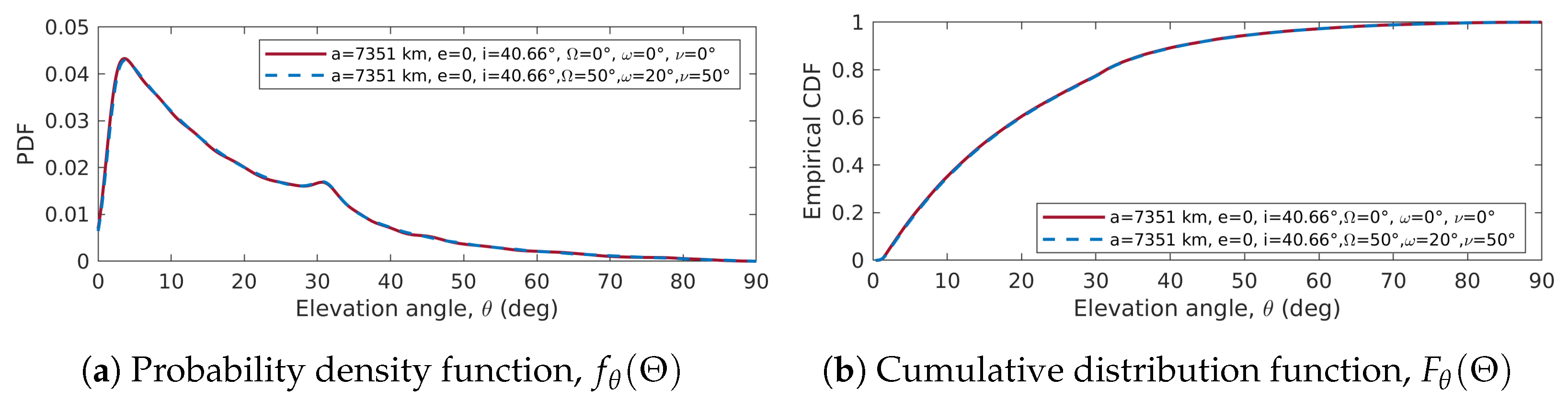
4.1.1. Effects of the Orbit Configuration in the Elevation Angle Distribution

The Kepler orbital elements were chosen to describe the orbits, those parameters include the semi-major axis, a, eccentricity, e, orbit inclination, i, right ascension of the ascending node, Ω , argument of perigee, ω , and true anomaly, ν . The values of the right ascension of the ascending node, Ω , argument of perigee, ω , and true anomaly, ν , do not affect the statistical properties of the elevation angle, then, those values are not further discussed. Figure 12a,b show the PDF and CDF elevation angle curves observed from the same location for two simulated satellites with different orbit configurations which share the same initial semi-major axis, a, eccentricity, e, and orbit inclination, i; but, differ in the initial values of the right ascension of the ascending node, Ω , argument of perigee, ω , and of the true anomaly, ν .

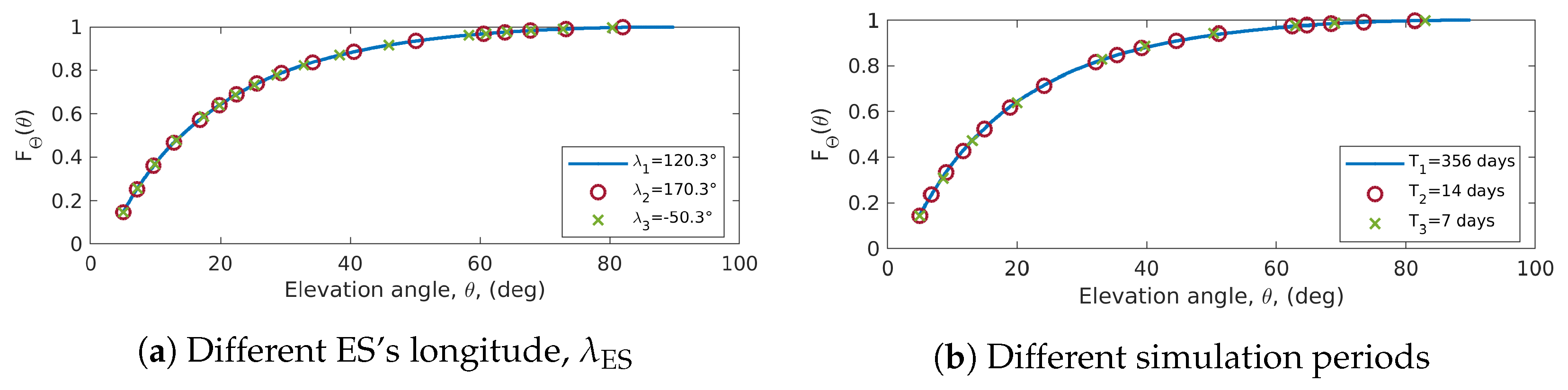
4.1.2. Elevation Angle CDF for Different Longitudes

ES’s located at different longitudes share approximately the same elevation angle distribution for the same LEO satellite configuration. The reasoning behind this fact is discussed in [2], and it is illustrated in Figure 13a, which shows the elevation angle PDF for three ES’s located at the same latitude, ϕ , but at different longitudes, λ ’s. Figure 13a shows that the elevation angle PDF is the same for ES located at different longitudes, λ ’s, when they share the same latitude, ϕ , and those are served by satellites with the same orbit configuration (semi-major axis, a, eccentricity, e, and, inclination, i). The PDF’s shown in Figure 13a were generated for a satellite with a circular orbit and an inclination of i = 60 ° , and an altitude of h = 1800 km; in addition, all ES’s were located at the same latitude ϕ = 25 ° N.

4.1.3. Long Term Validity of f Θ ( θ ) and F Θ ( θ )

From a few days f Θ ( θ ) can be observed very similar compared with the same PDF is a much greater period, e.g., one year. Figure 13b shows the functions F Θ ( θ ) for three different simulation periods ranging from one week to one year. The CDF curve is almost identical for all the simulation periods. The orbit configuration and ES’s location were choose to be the same that for Figure 13a.

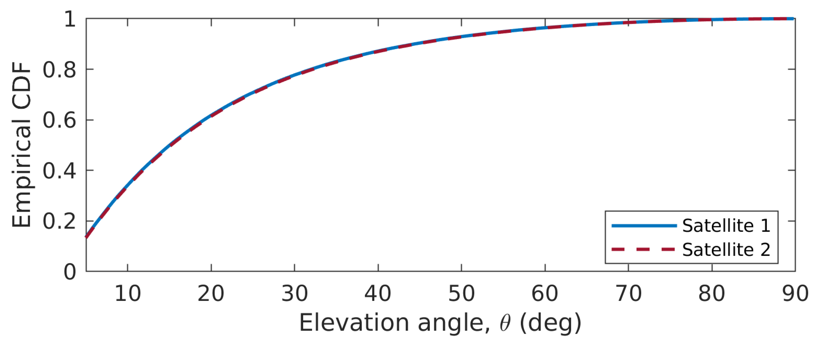
4.1.4. Elevation Angle CDF for Different Satellite Characteristics
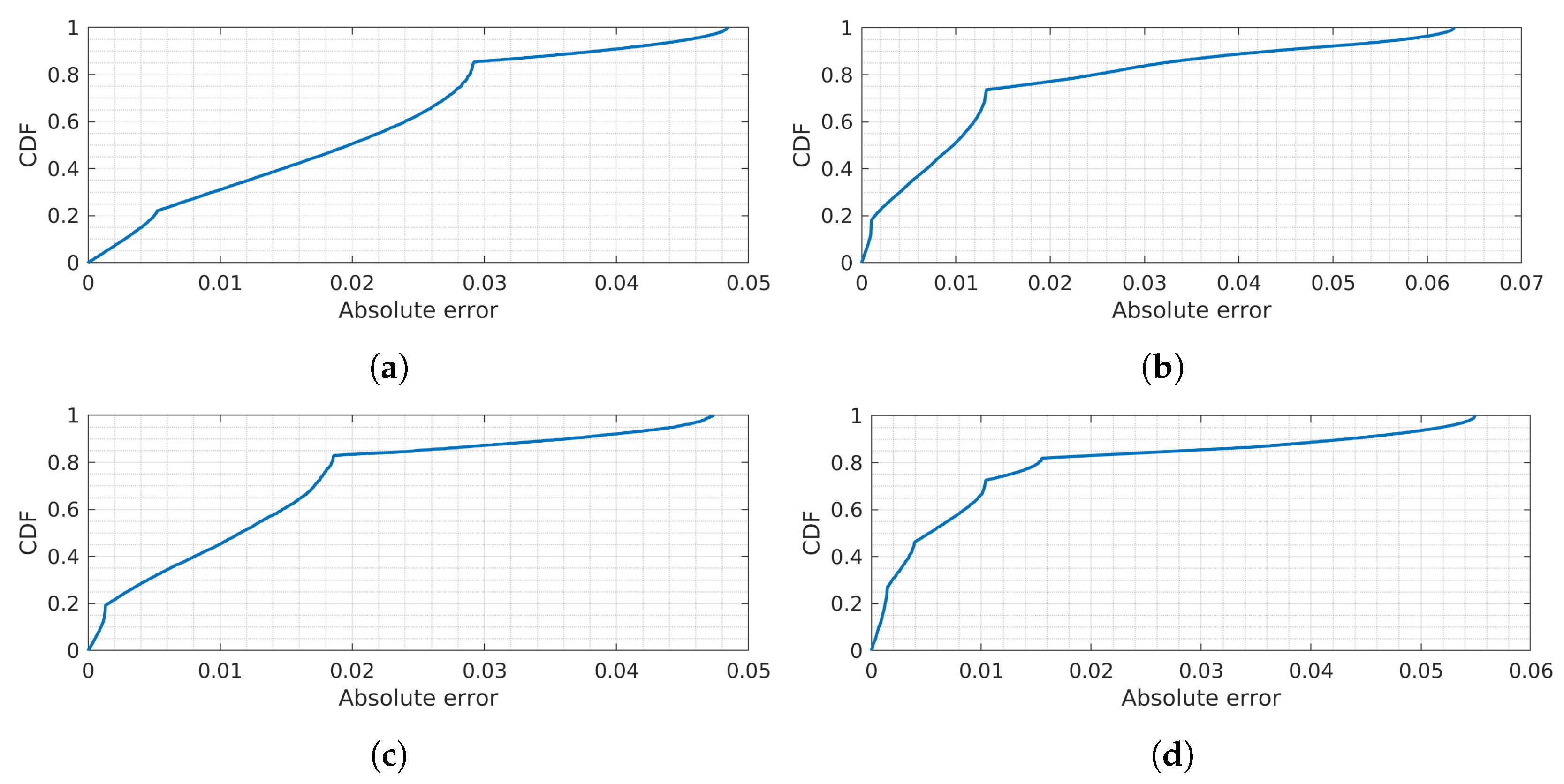
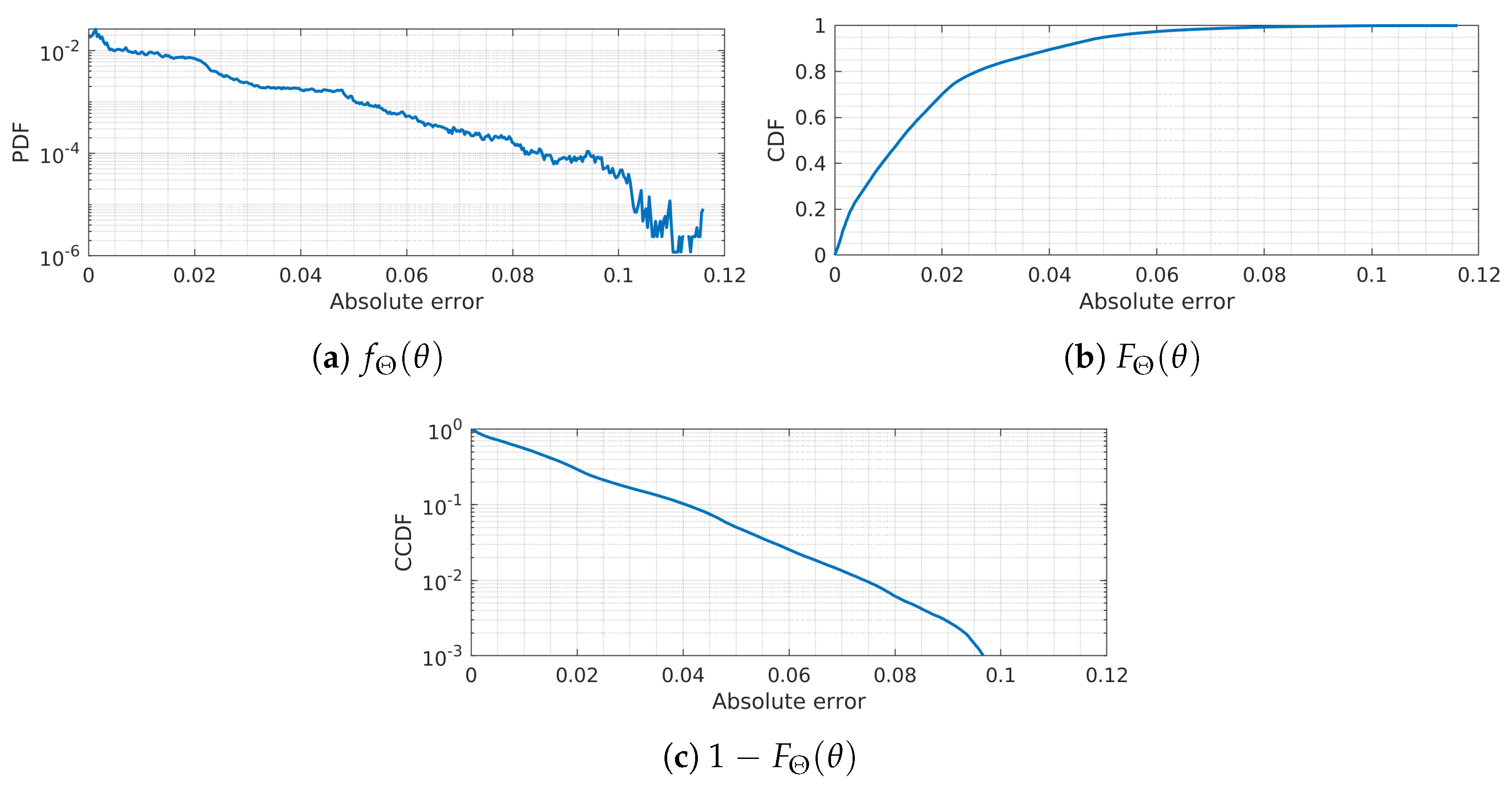
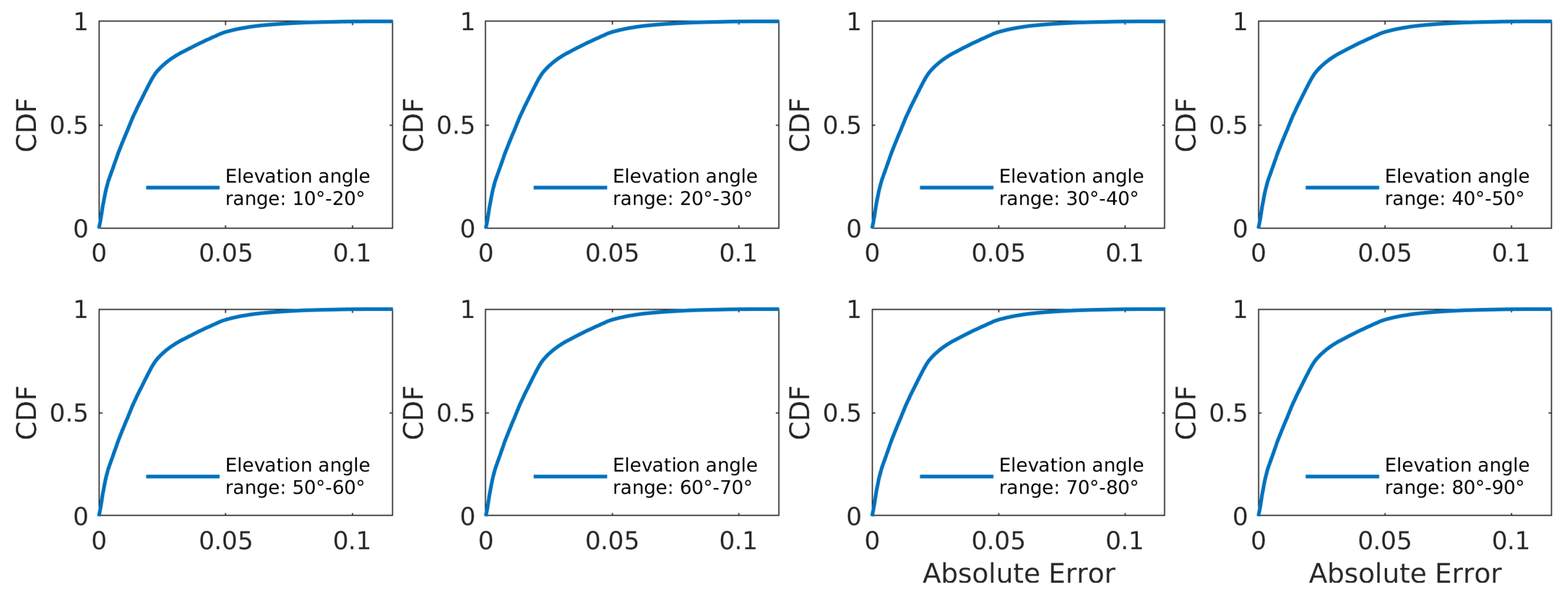
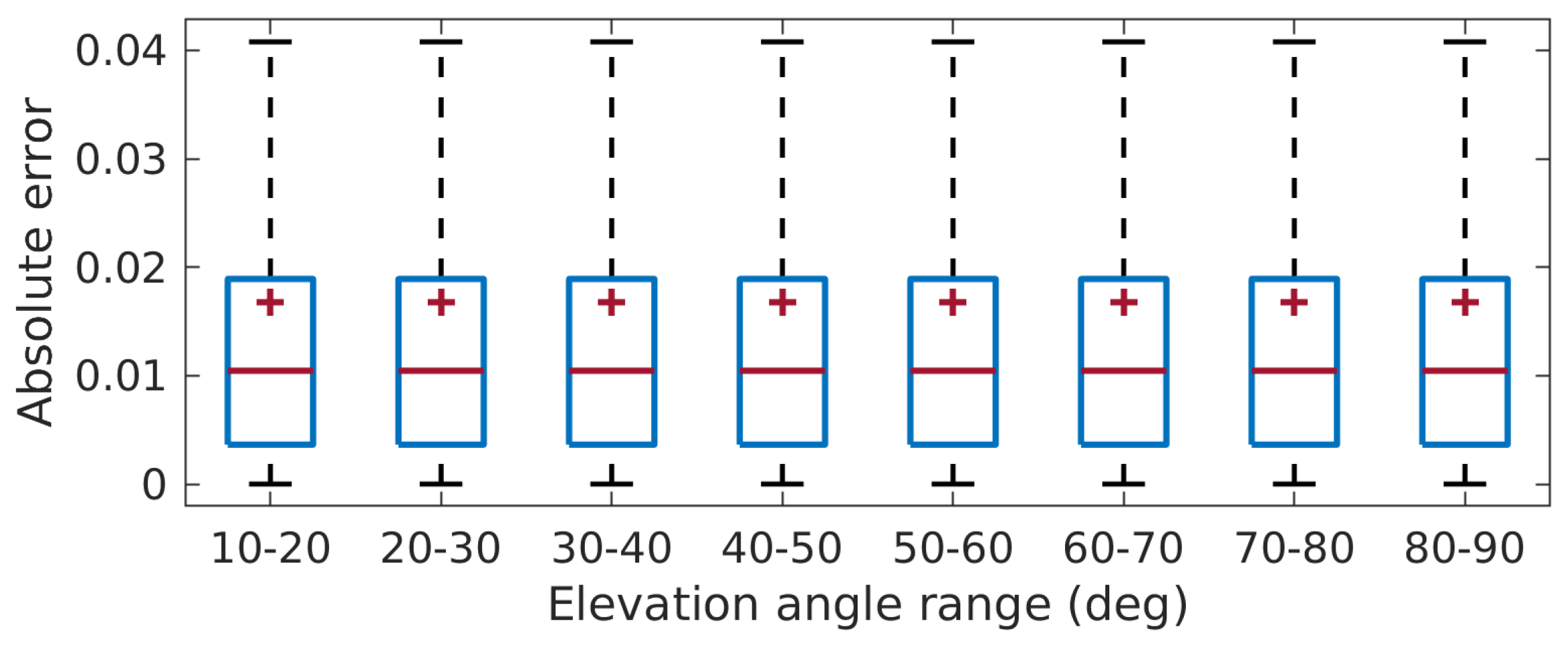
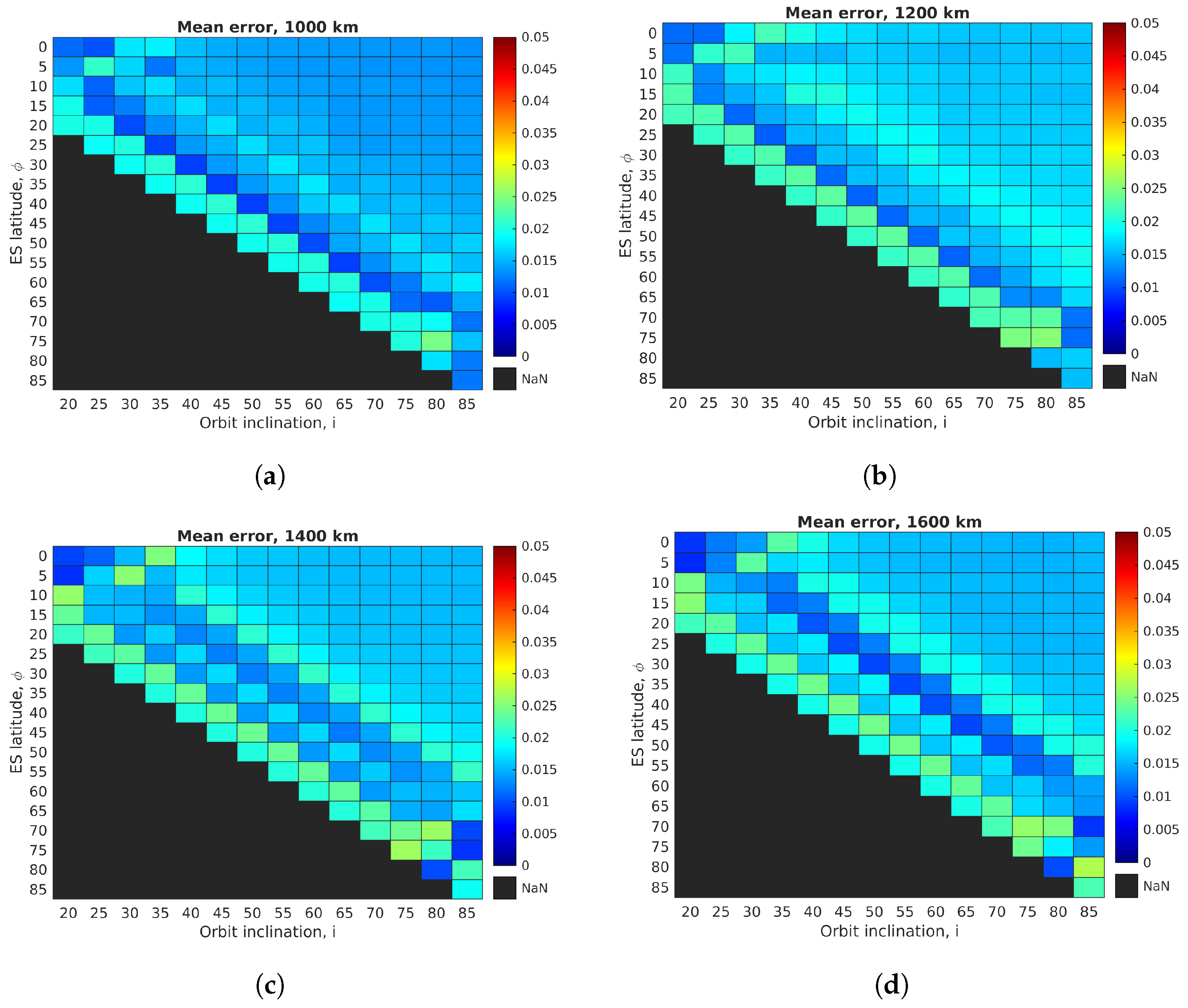
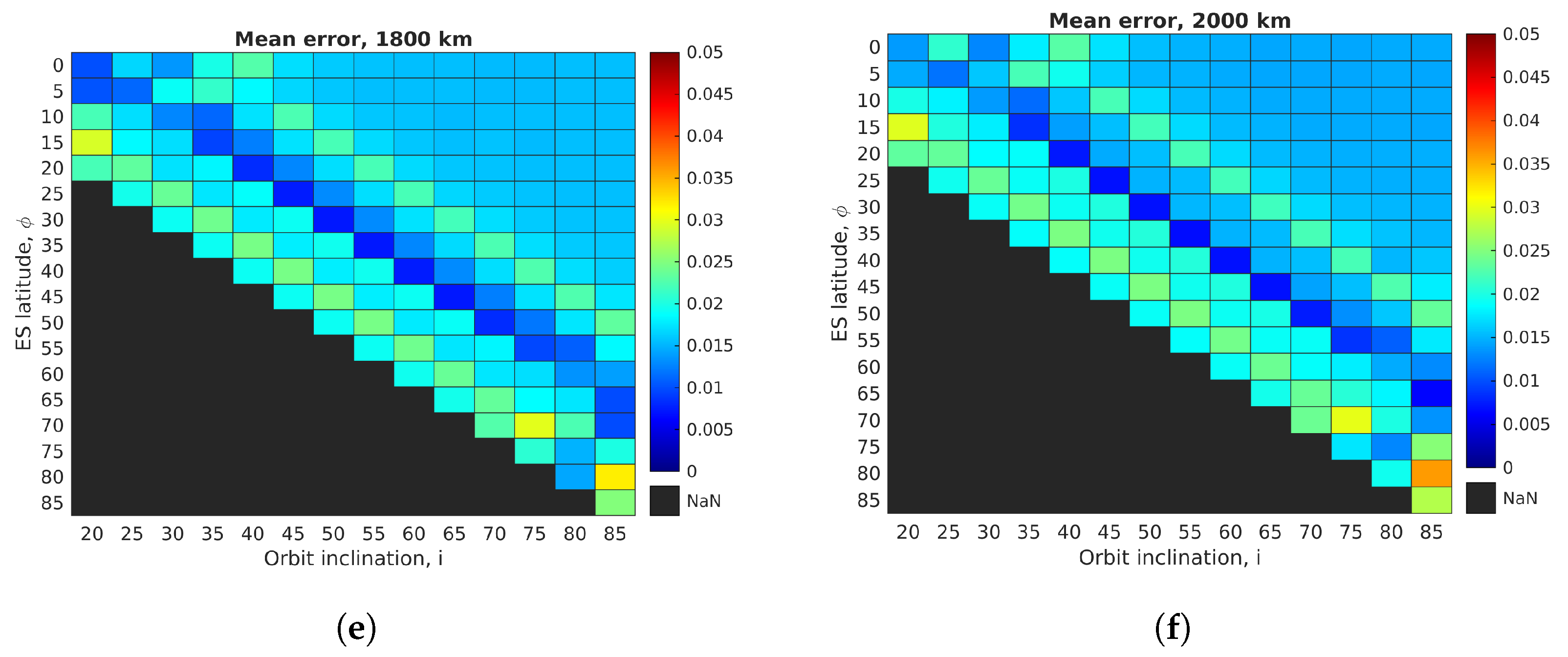
Simulations for this paper where performed for a satellite with the mass and drag areas listed in Table 1, nonetheless, satellites with different values in those characteristics will share very similar functions F Θ ( θ ) . Figure 14 shows the empirical CDF’s for two satellites with the same orbital parameters but with different mass and drag areas. For both satellites, the orbit altitude, h, was set to 1800 km and the orbit inclination, i, to 60 ° , and both ES’s were located at 25 ° N. As shown in Figure 14, variations in the satellite mass and drag area characteristics will have a very little impact in the elevation angle CDF’s. For lower altitudes the effect is greater, but not significant enough for the altitudes covered in this paper. Table 10 show the mass and areas for satellites shown in Figure 14.

4.2. Error Analysis

The error between the empirical CDF curves of the elevation angle and the ones obtained with the parameters in Table 6 and Table 7, was quantified by means of the absolute error, ϵ , and its CDF. Figure A1a–f in Appendix A show the mean absolute error, ϵ ¯ , between the empirical CDF’s for the simulated points of Figure 9c, and for the orbit altitudes h k h s .
The maximum observed mean error for the individual characterizations shown in Appendix A was about 5% ( ϵ ¯ m a x 0.05 ) for the worst case. However, the greatest error values were observed to occur at lower elevation angles (below 20 ° were the link is often unreliable since line-of-sight is harder to find) that are often not considered by satellite communication systems due to greater attenuation.
The absolute errors ϵ were also analyzed through their individual CDF’s, showing that most of the errors where below 5%. Figure 15a–d show the CDF’s of the absolute error, ϵ , corresponding to Figure 10a–d. In addition, ϵ was analyzed for all the simulated satellite orbits and according to their elevation angle range.
The PDF, CDF, and the complementary CDF (CCDF) showing the resultant absolute errors, ϵ , for all the simulations are shown in Figure 16, where it can be observed that around 95% of the values of ϵ are below 0.05. Figure 17 shows the same absolute errors as in Figure 16b, but now expanded and classified by elevation angle range; in this figure, it can be observed that most of the absolute errors are below 5% for all the elevation angle ranges, and that errors’ CDF distributions are approximately the same for all the elevation angle ranges. Figure 18 expands the 90th-percentile of the CDF’s in Figure 17, showing that in fact, most of the errors are below 2%; the 90th-percentile mean value is shown as a red cross for each boxplot.

5. Conclusions

This article demonstrated the feasibility of using a gamma random variable to characterize the elevation angle PDF and CDF. The proposed methodology allowed PDF and CDF calculations of the elevation angle for LEO satellites for altitudes between 1000 km and 2000 km. The characterization of elevation angle through a gamma random variable allowed an easy computation of first and second order statistics, which, to the best of our knowledge, have not been previously addressed in the literature.
The proposed methodology was validated with an error analysis against the empirical CDF’s. The results showed that errors are low, with a mean absolute error much below 5% in most of the cases, and with around 95% of the total errors being below 5%.
Furthermore, the proposed methodology allows an easy comparison between multiple orbits in order to determine the most suitable orbital parameters to provide coverage above a minimum elevation angle at a particular latitude.

Author Contributions

Conceptualization, J.M.G.-T. and C.V.-R.; methodology and software, J.M.G.-T.; validation, A.A.-Z. and R.V.-H.; formal analysis, A.A.-Z. and R.V.-H.; investigation, A.A.-Z. and R.V.-H.; writing—original draft preparation, J.M.G.-T.; writing—review and editing, C.V.-R., A.A.-Z. and R.V.-H.; visualization, J.M.G.-T.; supervision, J.M.G.-T., C.V.-R. and A.A.-Z.; project administration, C.V.-R. and R.V.-H. All authors have read and agreed to the published version of the manuscript.

Funding

This research received no external funding.

Institutional Review Board Statement

Not applicable.

Informed Consent Statement

Not applicable.

Data Availability Statement

Not applicable.

Acknowledgments

We would like to acknowledge the support from the Smart Digital Technologies and Infrastructure Research Group, the project “Digital Technologies to Create Adaptive Smart Cities” as part of the Challenge-Based Research Funding Program, and the School of Engineering and Sciences at Tecnologico de Monterrey for providing the means to develop this collaborative work.

Conflicts of Interest

The authors declare no conflict of interest.

Abbreviations

The following abbreviations are used in this manuscript:
CDFCumulative distribution function
CCDFComplementary cumulative distribution function
ESEarth station
GEOGeostationary Earth orbit
LEOLow Earth orbit
LMSLand mobile satellite
LOSLine-of-sight
NGEONon-Geostationary Earth orbit
NGSONon-Geosynchronous orbit
NLOSNon-line-of-sight
PDFProbability density function

Appendix A

Figure A1a–f contain the mean error for each elevation angle CDF. Those errors were obtained by comparing the proposed methodology results against the results obtained through simulations. The same format than in Figure 9c,d is applied here; only showing the ES’s located below the satellite orbit inclinations at each column.
Figure A1. Mean error obtained with the proposed methodology, as compared with the simulation results for all the simulated orbit inclinations, i S A T , ES’s latitudes, ϕ E S , and altitudes, h k . (a) Proposed methodology vs simulations results at 1000 km; (b) Proposed methodology vs simulations results at 1200 km; (c) Proposed methodology vs simulations results at 1400 km; (d) Proposed methodology vs simulations results at 1600 km; (e) Proposed methodology vs simulations results at 1800 km; (f) Proposed methodology vs simulations results at 2000 km.
Applsci 13 04405 g0a1aApplsci 13 04405 g0a1b

Appendix B

Table A1, Table A2, Table A3, Table A4, Table A5 and Table A6 contain the shape, a, and rate, b, parameters for f Θ ( θ ) at the simulated values of i and ϕ . With those results, matrices A h and B h are formed as defined in (17) and depicted in Figure 9d. Also, Table A7 contains the numerical values for w a and w b .
Table A1. Shape, a, and rate, b parameter for f Θ ( θ ) and F Θ ( θ ) for h k = 1000 km.
Shape parameter, a
Orbit inclination, i
20 ° 25 ° 30 ° 35 ° 40 ° 45 ° 50 ° 55 ° 60 ° 65 ° 70 ° 75 ° 80 ° 85 °
ES latitude, ϕ 0 ° 1.60631.58461.46591.43451.45841.47421.48171.48541.48641.49761.49811.49901.49541.5031
5 ° 1.76621.48531.41511.45481.46671.47701.48591.48981.49661.49681.49781.50151.50171.5040
10 ° 1.50361.62701.62911.46891.43031.46461.47561.47851.47791.49561.48671.49361.49351.4983
15 ° 1.39461.55701.65951.63901.46491.43401.46181.46901.47241.49381.49211.49141.48811.4920
20 ° 1.37491.42201.56881.66891.63821.46801.43071.45451.45731.48911.48481.48511.48281.4832
25 ° NaN1.39441.43321.57761.67201.64771.46761.42521.44741.48541.48921.48031.47761.4816
30 ° NaNNaN1.39251.43691.57631.67711.64281.45731.40841.47331.46771.47151.47021.4730
35 ° NaNNaNNaN1.39251.43471.58151.67561.63541.44261.44461.46081.46411.46221.4682
40 ° NaNNaNNaNNaN1.39051.43801.57861.66691.61891.48311.42731.45261.45541.4612
45 ° NaNNaNNaNNaNNaN1.39401.43561.57081.64511.66051.46631.42211.44441.4527
50 ° NaNNaNNaNNaNNaNNaN1.39101.42711.55501.68941.63671.46081.41211.4398
55 ° NaNNaNNaNNaNNaNNaNNaN1.38241.41001.58941.66251.62761.45071.4099
60 ° NaNNaNNaNNaNNaNNaNNaNNaN1.36601.44351.56371.64661.60551.4458
65 ° NaNNaNNaNNaNNaNNaNNaNNaNNaN1.40011.41731.54111.60721.5573
70 ° NaNNaNNaNNaNNaNNaNNaNNaNNaNNaN1.37341.38931.46561.5816
75 ° NaNNaNNaNNaNNaNNaNNaNNaNNaNNaNNaN1.31801.36041.6773
80 ° NaNNaNNaNNaNNaNNaNNaNNaNNaNNaNNaNNaN1.53591.6471
85 ° NaNNaNNaNNaNNaNNaNNaNNaNNaNNaNNaNNaNNaN1.6787
Rate parameter, b × 10 2
Orbit inclination, i
20 ° 25 ° 30 ° 35 ° 40 ° 45 ° 50 ° 55 ° 60 ° 65 ° 70 ° 75 ° 80 ° 85 °
ES latitude, ϕ 0 ° 9.35649.75869.50668.95698.87118.85678.83808.81938.80298.82608.81548.80868.78658.8199
5 ° 10.540310.00619.05498.95358.87638.85448.84698.83178.83548.82318.81588.82088.81558.8212
10 ° 7.76068.99779.80079.46618.88948.87418.84518.81168.78058.82448.77528.79498.78368.8062
15 ° 6.62197.76339.04289.81249.43428.89828.85598.81288.78698.83878.82028.80298.78168.7902
20 ° 6.65646.60327.74379.04799.79379.45318.88828.82378.76898.84368.80788.78848.76998.7666
25 ° NaN6.63266.58417.74029.03629.83539.45838.86488.80238.86718.84348.78748.76288.7717
30 ° NaNNaN6.58396.56807.71449.05899.82369.42448.80838.89318.80748.78328.75538.7587
35 ° NaNNaNNaN6.55676.54107.73129.05489.79859.37068.94068.85348.79898.75588.7643
40 ° NaNNaNNaNNaN6.53046.55137.72299.02679.74589.51968.88118.82828.77538.7717
45 ° NaNNaNNaNNaNNaN6.54346.54597.70168.95859.87909.45848.86958.80888.7893
50 ° NaNNaNNaNNaNNaNNaN6.54106.52957.66659.09709.79839.44118.84418.8240
55 ° NaNNaNNaNNaNNaNNaNNaN6.53066.49757.76889.02349.77349.40878.8794
60 ° NaNNaNNaNNaNNaNNaNNaNNaN6.50956.60647.72258.99479.71219.4440
65 ° NaNNaNNaNNaNNaNNaNNaNNaNNaN6.64206.58457.70798.92629.6598
70 ° NaNNaNNaNNaNNaNNaNNaNNaNNaNNaN6.65496.60897.63399.2649
75 ° NaNNaNNaNNaNNaNNaNNaNNaNNaNNaNNaN6.72006.98758.5786
80 ° NaNNaNNaNNaNNaNNaNNaNNaNNaNNaNNaNNaN7.70017.3090
85 ° NaNNaNNaNNaNNaNNaNNaNNaNNaNNaNNaNNaNNaN6.6598
Table A2. Shape, a, and rate, b parameter for f Θ ( θ ) and F Θ ( θ ) for h k = 1200 km.
Shape parameter, a
Orbit inclination, i
20 ° 25 ° 30 ° 35 ° 40 ° 45 ° 50 ° 55 ° 60 ° 65 ° 70 ° 75 ° 80 ° 85 °
ES latitude, ϕ 0 ° 1.93671.84761.78391.68681.69551.74171.74091.74921.74471.75971.75911.76011.76341.7602
5 ° 2.11771.85211.63271.70801.70981.74861.74881.75581.76081.76941.77141.76501.77161.7719
10 ° 1.69261.89591.93051.80021.67021.71411.73761.74311.74301.75891.75691.75781.75701.7563
15 ° 1.62071.78631.91541.95341.77771.64951.72121.73171.73641.75571.75621.75391.75871.7589
20 ° 1.60951.64901.81631.93461.93981.79801.65581.71631.72351.75141.74771.75071.74651.7494
25 ° NaN1.62321.66271.79971.93601.95441.79831.65581.70681.74901.74321.74791.74881.7452
30 ° NaNNaN1.62521.68721.82151.94921.95481.79311.63751.73211.73371.73921.73431.7354
35 ° NaNNaNNaN1.64471.66181.82211.95371.95121.78071.67481.71771.72721.73251.7302
40 ° NaNNaNNaNNaN1.62251.66011.82401.94601.93661.81351.65601.71601.72351.7234
45 ° NaNNaNNaNNaNNaN1.62541.66331.81641.93221.97021.79781.65281.70791.7157
50 ° NaNNaNNaNNaNNaNNaN1.62381.65431.80211.96261.94881.79521.64781.6998
55 ° NaNNaNNaNNaNNaNNaNNaN1.61631.64311.83011.93661.93941.78641.6401
60 ° NaNNaNNaNNaNNaNNaNNaNNaN1.60511.66661.80281.92301.91781.7669
65 ° NaNNaNNaNNaNNaNNaNNaNNaNNaN1.62961.64021.78101.87671.8103
70 ° NaNNaNNaNNaNNaNNaNNaNNaNNaNNaN1.60071.60941.65901.9132
75 ° NaNNaNNaNNaNNaNNaNNaNNaNNaNNaNNaN1.50391.65021.9769
80 ° NaNNaNNaNNaNNaNNaNNaNNaNNaNNaNNaNNaN1.83881.9151
85 ° NaNNaNNaNNaNNaNNaNNaNNaNNaNNaNNaNNaNNaN1.9243
Rate parameter, b × 10 2
Orbit inclination, i
20 ° 25 ° 30 ° 35 ° 40 ° 45 ° 50 ° 55 ° 60 ° 65 ° 70 ° 75 ° 80 ° 85 °
ES latitude, ϕ 0 ° 9.867810.117210.18919.52619.27939.37299.30729.30669.24769.29199.27639.26679.26739.2552
5 ° 10.949010.79769.53969.46179.47029.40779.33399.32329.31459.34249.33829.28789.31869.3206
10 ° 7.97559.307310.184810.27979.50519.34389.33309.30519.26269.29739.27739.26549.25279.2481
15 ° 7.01898.01879.251110.248710.02209.30579.35999.30839.27449.31049.30029.27069.28909.2896
20 ° 7.10706.96678.03539.365610.240910.15719.34729.34019.27729.32229.28139.27499.24389.2536
25 ° NaN7.04706.95147.91659.303410.235310.16219.35599.29979.35859.29609.28459.26569.2505
30 ° NaNNaN7.00186.96597.99539.321410.244310.14699.29109.39129.31409.28759.23999.2356
35 ° NaNNaNNaN7.03946.89848.00229.339210.228610.10829.42099.34999.29779.26959.2465
40 ° NaNNaNNaNNaN6.95216.89187.99919.317410.189510.20729.36789.34879.29349.2639
45 ° NaNNaNNaNNaNNaN6.95736.90047.98589.282710.275710.16399.35849.33289.2961
50 ° NaNNaNNaNNaNNaNNaN6.95896.88517.95379.361210.221010.15269.35839.3438
55 ° NaNNaNNaNNaNNaNNaNNaN6.95456.87288.03769.304510.198210.13799.3821
60 ° NaNNaNNaNNaNNaNNaNNaNNaN6.95386.95537.99659.295210.163410.1416
65 ° NaNNaNNaNNaNNaNNaNNaNNaNNaN7.06056.94408.00149.24149.9957
70 ° NaNNaNNaNNaNNaNNaNNaNNaNNaNNaN7.08266.98827.87429.7894
75 ° NaNNaNNaNNaNNaNNaNNaNNaNNaNNaNNaN7.12307.56698.9129
80 ° NaNNaNNaNNaNNaNNaNNaNNaNNaNNaNNaNNaN8.17807.6105
85 ° NaNNaNNaNNaNNaNNaNNaNNaNNaNNaNNaNNaNNaN6.9258
Table A3. Shape, a, and rate, b parameter for f Θ ( θ ) and F Θ ( θ ) for h k = 1400 km.
Shape parameter, a
Orbit inclination, i
20 ° 25 ° 30 ° 35 ° 40 ° 45 ° 50 ° 55 ° 60 ° 65 ° 70 ° 75 ° 80 ° 85 °
ES latitude, ϕ 0 ° 2.00321.84561.84021.67161.71001.73401.74491.75111.75431.76371.76321.76511.77021.7679
5 ° 2.16551.97541.65221.69341.72311.74091.74901.75401.75911.76141.76491.76631.76671.7666
10 ° 1.66771.89921.94351.86571.67211.71271.73531.74361.74991.75991.75881.76211.75861.7636
15 ° 1.60881.74241.91011.96361.87291.67051.71341.73231.73931.75621.75431.75681.76751.7563
20 ° 1.62031.69621.79521.92951.97411.87641.67011.70791.72691.75061.74811.75271.75481.7517
25 ° NaN1.59761.66511.80751.94021.98171.88011.66631.70241.74271.74211.74981.73271.7498
30 ° NaNNaN1.63691.66351.81081.94131.98141.87361.65731.71781.72951.74041.74021.7417
35 ° NaNNaNNaN1.64451.67151.81271.94341.97631.86651.67781.70501.73021.74231.7363
40 ° NaNNaNNaNNaN1.64561.67181.81171.93781.96731.88691.66501.70611.72061.7275
45 ° NaNNaNNaNNaNNaN1.64491.67101.80751.92791.98851.87151.66851.70481.7163
50 ° NaNNaNNaNNaNNaNNaN1.64401.66451.79681.94661.96681.87001.66891.6933
55 ° NaNNaNNaNNaNNaNNaNNaN1.63681.65381.81181.92171.95821.85821.6591
60 ° NaNNaNNaNNaNNaNNaNNaNNaN1.62651.66841.78681.90541.93261.8204
65 ° NaNNaNNaNNaNNaNNaNNaNNaNNaN1.64031.64141.76111.84771.8296
70 ° NaNNaNNaNNaNNaNNaNNaNNaNNaNNaN1.60741.59701.65741.9844
75 ° NaNNaNNaNNaNNaNNaNNaNNaNNaNNaNNaN1.53021.74002.0124
80 ° NaNNaNNaNNaNNaNNaNNaNNaNNaNNaNNaNNaN1.90511.9381
85 ° NaNNaNNaNNaNNaNNaNNaNNaNNaNNaNNaNNaNNaN1.9298
Rate parameter, b × 10 2
Orbit inclination, i
20 ° 25 ° 30 ° 35 ° 40 ° 45 ° 50 ° 55 ° 60 ° 65 ° 70 ° 75 ° 80 ° 85 °
ES latitude, ϕ 0 ° 9.48549.65879.93849.31169.07289.03178.99698.97568.95838.96618.94888.94408.95348.9475
5 ° 10.329510.65089.60709.15469.06259.03098.99898.97768.96758.95468.95158.94608.93558.9351
10 ° 7.66748.84359.66899.92369.25959.04979.00658.97478.95888.96348.94298.93968.92088.9386
15 ° 6.79327.52278.73349.67909.92239.25049.03948.99008.95628.97318.94248.93488.95868.9182
20 ° 6.94806.86147.60018.74929.68869.93829.24939.01968.97038.98738.94508.94088.93278.9139
25 ° NaN6.77566.72667.59538.75319.71309.94969.23459.00019.01678.95948.95428.87468.9231
30 ° NaNNaN6.83076.68797.57958.75579.71149.92989.20929.04798.97798.96168.92928.9203
35 ° NaNNaNNaN6.82016.68737.58028.75759.69349.91059.27429.01048.98808.97108.9328
40 ° NaNNaNNaNNaN6.80466.68377.57558.74209.67089.96759.23629.02378.96548.9487
45 ° NaNNaNNaNNaNNaN6.80136.68347.56818.71969.72699.92199.25399.02928.9823
50 ° NaNNaNNaNNaNNaNNaN6.80586.67607.55108.77279.67069.92259.26619.0351
55 ° NaNNaNNaNNaNNaNNaNNaN6.80306.66717.60178.72339.66009.89919.2876
60 ° NaNNaNNaNNaNNaNNaNNaNNaN6.80556.73067.57438.71679.62559.8749
65 ° NaNNaNNaNNaNNaNNaNNaNNaNNaN6.88986.72597.58508.66059.6210
70 ° NaNNaNNaNNaNNaNNaNNaNNaNNaNNaN6.91556.76577.63659.4222
75 ° NaNNaNNaNNaNNaNNaNNaNNaNNaNNaNNaN7.14597.52838.4633
80 ° NaNNaNNaNNaNNaNNaNNaNNaNNaNNaNNaNNaN7.94487.2608
85 ° NaNNaNNaNNaNNaNNaNNaNNaNNaNNaNNaNNaNNaN6.6159
Table A4. Shape, a, and rate, b parameter for f Θ ( θ ) and F Θ ( θ ) for h k = 1600 km.
Shape parameter, a
Orbit inclination, i
20 ° 25 ° 30 ° 35 ° 40 ° 45 ° 50 ° 55 ° 60 ° 65 ° 70 ° 75 ° 80 ° 85 °
ES latitude, ϕ 0 ° 2.05121.92351.85371.74061.68441.73331.74501.75371.75701.76181.76301.76561.76891.7680
5 ° 2.19422.06071.77171.66011.71641.73881.75081.75581.76131.76471.76771.77011.76811.7687
10 ° 1.73091.81641.94091.91051.74461.69081.73361.74641.75001.75901.75801.76201.76571.7720
15 ° 1.58531.75491.89681.97011.91551.75281.68971.73091.74021.75911.75631.76071.76041.7762
20 ° 1.62391.65321.78861.91841.97761.93041.75231.68781.72791.75221.75381.75911.75731.7647
25 ° NaN1.64891.67241.79931.92371.99101.93251.75121.68461.73951.74501.75401.75501.7582
30 ° NaNNaN1.65471.67541.79841.93301.99351.93171.74731.69701.72911.74401.74781.7502
35 ° NaNNaNNaN1.65601.67151.80621.93261.98931.92351.75781.68381.72671.73761.7407
40 ° NaNNaNNaNNaN1.65261.67891.80521.93021.98151.93651.74651.68361.72371.7222
45 ° NaNNaNNaNNaNNaN1.66061.67941.80261.92241.99431.92111.74831.68181.7154
50 ° NaNNaNNaNNaNNaNNaN1.65901.67531.79361.93161.97361.91561.74571.6728
55 ° NaNNaNNaNNaNNaNNaNNaN1.65501.66601.80101.90811.96101.90261.7332
60 ° NaNNaNNaNNaNNaNNaNNaNNaN1.64501.67301.77521.88661.92761.8312
65 ° NaNNaNNaNNaNNaNNaNNaNNaNNaN1.65091.64251.74221.79731.9083
70 ° NaNNaNNaNNaNNaNNaNNaNNaNNaNNaN1.61071.56871.72322.0355
75 ° NaNNaNNaNNaNNaNNaNNaNNaNNaNNaNNaN1.61651.80792.0373
80 ° NaNNaNNaNNaNNaNNaNNaNNaNNaNNaNNaNNaN1.94951.9564
85 ° NaNNaNNaNNaNNaNNaNNaNNaNNaNNaNNaNNaNNaN1.9366
Rate parameter, b × 10 2
Orbit inclination, i
20 ° 25 ° 30 ° 35 ° 40 ° 45 ° 50 ° 55 ° 60 ° 65 ° 70 ° 75 ° 80 ° 85 °
ES latitude, ϕ 0 ° 9.13429.51749.59449.31358.78188.78078.74268.72238.69598.68818.67418.67428.67428.6766
5 ° 9.796610.37529.78818.88428.81108.77468.74748.71928.70388.69578.69058.68678.66858.6762
10 ° 7.62748.22799.20229.63819.26928.76748.75678.72678.68958.68868.66478.66708.66928.6931
15 ° 6.60807.30628.29889.22309.62879.29058.75388.73768.69388.71738.68218.67888.66268.7096
20 ° 6.81796.59017.30078.30619.21759.66599.28478.74658.72478.73388.70248.69348.66638.6864
25 ° NaN6.75666.56957.28548.30009.24859.67239.28338.73618.75998.71288.70188.67858.6748
30 ° NaNNaN6.71366.53837.26238.31509.25369.67159.27198.77498.73198.71078.68418.6771
35 ° NaNNaNNaN6.68236.50957.27208.31009.24169.64689.30388.74088.72848.69698.6821
40 ° NaNNaNNaNNaN6.65786.52037.26618.30219.22099.68209.27268.74548.72688.6719
45 ° NaNNaNNaNNaNNaN6.67516.52347.26108.28859.25509.63939.28088.74968.7354
50 ° NaNNaNNaNNaNNaNNaN6.67816.52077.25268.31779.20609.62859.28328.7699
55 ° NaNNaNNaNNaNNaNNaNNaN6.68276.52007.28688.27739.18999.61239.3061
60 ° NaNNaNNaNNaNNaNNaNNaNNaN6.69216.56797.26258.26509.15239.5221
65 ° NaNNaNNaNNaNNaNNaNNaNNaNNaN6.76006.56197.26858.16129.4608
70 ° NaNNaNNaNNaNNaNNaNNaNNaNNaNNaN6.78136.56647.59909.0780
75 ° NaNNaNNaNNaNNaNNaNNaNNaNNaNNaNNaN7.27017.44588.0980
80 ° NaNNaNNaNNaNNaNNaNNaNNaNNaNNaNNaNNaN7.71616.9900
85 ° NaNNaNNaNNaNNaNNaNNaNNaNNaNNaNNaNNaNNaN6.3842
Table A5. Shape, a, and rate, b parameter for f Θ ( θ ) and F Θ ( θ ) for h k = 1800 km.
Shape parameter, a
Orbit inclination, i
20 ° 25 ° 30 ° 35 ° 40 ° 45 ° 50 ° 55 ° 60 ° 65 ° 70 ° 75 ° 80 ° 85 °
ES latitude, ϕ 0 ° 2.08641.98841.81691.79431.64121.72481.74381.75501.76091.76641.77141.77071.77031.7721
5 ° 2.21162.12131.87641.58971.70651.73681.75131.75991.76451.76651.77471.77421.77481.7745
10 ° 1.79231.73481.92701.93371.81421.64121.72691.74681.75391.76551.76191.76801.76761.7691
15 ° 1.52971.73561.88211.96641.95191.81801.63891.72781.74451.75761.75431.76421.76551.7646
20 ° 1.62391.65651.77791.90411.97971.95921.81911.63881.72491.74731.75101.75771.76011.7588
25 ° NaN1.65911.67671.79151.91671.99111.96491.82311.63611.73071.74621.75161.75531.7561
30 ° NaNNaN1.66761.68101.79851.92041.99361.96581.81621.64171.72181.73921.74782.1573
35 ° NaNNaNNaN1.67091.68701.80071.92381.99591.96081.82651.63291.71941.73632.6343
40 ° NaNNaNNaNNaN1.67241.68791.80111.92401.99031.96881.81551.63321.71641.7308
45 ° NaNNaNNaNNaNNaN1.67461.68761.80101.91561.99491.95411.81301.63341.7091
50 ° NaNNaNNaNNaNNaNNaN1.67311.68551.79261.92011.97431.94511.80601.6291
55 ° NaNNaNNaNNaNNaNNaNNaN1.67001.67761.79291.89431.95801.92341.7826
60 ° NaNNaNNaNNaNNaNNaNNaNNaN1.66031.67601.76821.86971.90931.7970
65 ° NaNNaNNaNNaNNaNNaNNaNNaNNaN1.65851.64421.72191.71711.9728
70 ° NaNNaNNaNNaNNaNNaNNaNNaNNaNNaN1.60971.51731.78222.0709
75 ° NaNNaNNaNNaNNaNNaNNaNNaNNaNNaNNaN1.69511.85942.0537
80 ° NaNNaNNaNNaNNaNNaNNaNNaNNaNNaNNaNNaN1.97981.9692
85 ° NaNNaNNaNNaNNaNNaNNaNNaNNaNNaNNaNNaNNaN1.9458
Rate parameter, b × 10 2
Orbit inclination, i
20 ° 25 ° 30 ° 35 ° 40 ° 45 ° 50 ° 55 ° 60 ° 65 ° 70 ° 75 ° 80 ° 85 °
ES latitude, ϕ 0 ° 8.81969.33089.18619.25028.54898.56708.52938.50908.49078.48118.48128.46608.45188.4567
5 ° 9.346810.06769.83228.64498.60848.56858.53808.51648.49668.47958.49078.47668.46778.4626
10 ° 7.57957.75978.79759.33979.23878.50898.53968.51598.48818.48858.45978.46448.44938.4529
15 ° 6.40757.05477.95088.82519.35779.23678.48808.53188.50008.49248.45778.46798.45618.4484
20 ° 6.70476.46747.05367.94928.83219.37039.23558.48318.51738.50348.47018.46548.45478.4423
25 ° NaN6.65316.43847.03897.95458.85569.38189.24548.47468.53078.50318.47488.46068.4516
30 ° NaNNaN6.61116.41007.03277.95498.85699.38229.22658.49328.51078.48378.470411.6161
35 ° NaNNaNNaN6.58576.40367.02907.95788.86019.36969.25798.47098.50678.484617.2642
40 ° NaNNaNNaNNaN6.57146.40007.02627.95778.84819.39209.22598.47778.51068.4929
45 ° NaNNaNNaNNaNNaN6.57566.39907.03007.94168.86269.35309.22318.49278.5222
50 ° NaNNaNNaNNaNNaNNaN6.57696.40427.02087.96418.81859.33739.21728.5267
55 ° NaNNaNNaNNaNNaNNaNNaN6.58726.40447.04267.92268.79919.30549.2177
60 ° NaNNaNNaNNaNNaNNaNNaNNaN6.59486.43697.02827.91288.73709.1203
65 ° NaNNaNNaNNaNNaNNaNNaNNaNNaN6.65096.43757.01667.70569.2740
70 ° NaNNaNNaNNaNNaNNaNNaNNaNNaNNaN6.67026.38107.54458.7644
75 ° NaNNaNNaNNaNNaNNaNNaNNaNNaNNaNNaN7.33757.34307.7934
80 ° NaNNaNNaNNaNNaNNaNNaNNaNNaNNaNNaNNaN7.50426.7684
85 ° NaNNaNNaNNaNNaNNaNNaNNaNNaNNaNNaNNaNNaN6.2083
Table A6. Shape, a, and rate, b parameter for f Θ ( θ ) and F Θ ( θ ) for h k = 2000 km.
Shape parameter, a
Orbit inclination, i
20 ° 25 ° 30 ° 35 ° 40 ° 45 ° 50 ° 55 ° 60 ° 65 ° 70 ° 75 ° 80 ° 85 °
ES latitude, ϕ 0 ° 2.11332.04071.86631.82771.68511.71511.74341.75431.76341.76901.77301.77571.77471.7801
5 ° 2.22362.16641.96081.66231.69101.73281.75111.76011.76791.77421.77701.77791.77681.7844
10 ° 1.84641.76341.90541.94631.86271.68811.71801.74601.75681.77111.76791.77191.77181.7758
15 ° 1.57151.71521.86641.96101.97251.87021.68731.71891.74431.75741.76291.76691.76581.7698
20 ° 1.61761.65821.77171.89391.98241.98151.87331.68621.71531.74851.75281.75881.76121.7578
25 ° NaN1.66751.68271.78601.91111.99171.98781.87821.68671.71711.74211.75181.75591.7612
30 ° NaNNaN1.67811.68741.79721.91431.99361.98951.87451.68931.71041.73791.74531.7527
35 ° NaNNaNNaN1.67991.69631.79861.91701.99781.98671.87771.68191.70811.73171.7418
40 ° NaNNaNNaNNaN1.68831.69551.79931.92111.99091.98811.86741.68071.74531.7237
45 ° NaNNaNNaNNaNNaN1.68611.69551.79961.91181.99151.97461.86271.67811.6952
50 ° NaNNaNNaNNaNNaNNaN1.68491.69421.79251.90921.97151.96231.84991.6713
55 ° NaNNaNNaNNaNNaNNaNNaN1.68421.68701.78861.88571.95121.93121.8113
60 ° NaNNaNNaNNaNNaNNaNNaNNaN1.67401.68281.76091.85231.88201.8489
65 ° NaNNaNNaNNaNNaNNaNNaNNaNNaN1.66441.64631.69791.74742.0230
70 ° NaNNaNNaNNaNNaNNaNNaNNaNNaNNaN1.60261.56201.83302.0953
75 ° NaNNaNNaNNaNNaNNaNNaNNaNNaNNaNNaN1.76231.89992.0647
80 ° NaNNaNNaNNaNNaNNaNNaNNaNNaNNaNNaNNaN2.00231.9790
85 ° NaNNaNNaNNaNNaNNaNNaNNaNNaNNaNNaNNaNNaN1.9584
Rate parameter, b × 10 2
Orbit inclination, i
20 ° 25 ° 30 ° 35 ° 40 ° 45 ° 50 ° 55 ° 60 ° 65 ° 70 ° 75 ° 80 ° 85 °
ES latitude, ϕ 0 ° 8.54329.13999.09749.12028.59648.38818.36068.33188.31598.30148.29888.29448.28268.2926
5 ° 8.96989.77359.77938.83458.43128.39428.36408.33838.32388.32198.30998.30048.28468.3080
10 ° 7.51977.67518.44539.06079.13428.55908.36118.34528.31738.32858.29298.29018.27998.2844
15 ° 6.47486.85087.66608.49859.08729.13848.54298.35188.32608.31618.29668.28948.27118.2777
20 ° 6.60236.36756.86757.67078.51959.10229.14228.53598.33338.33638.29488.28408.27218.2523
25 ° NaN6.56656.34266.84867.68058.53409.11419.15468.53548.33738.31368.29508.27918.2811
30 ° NaNNaN6.52736.30996.84777.67858.53219.11639.14328.54778.31808.30658.28348.2823
35 ° NaNNaNNaN6.49356.30746.84227.67938.54049.10729.15468.52418.31798.29988.2902
40 ° NaNNaNNaNNaN6.49556.30036.84077.68958.52309.11289.12418.52738.28348.2992
45 ° NaNNaNNaNNaNNaN6.48916.30056.84387.67098.52939.08009.11678.53608.3301
50 ° NaNNaNNaNNaNNaNNaN6.49186.30656.83977.67628.49129.05909.10038.5634
55 ° NaNNaNNaNNaNNaNNaNNaN6.50686.31066.85297.64758.46809.01329.0711
60 ° NaNNaNNaNNaNNaNNaNNaNNaN6.51646.33916.83867.62428.37269.0403
65 ° NaNNaNNaNNaNNaNNaNNaNNaNNaN6.55716.34026.80447.62739.0766
70 ° NaNNaNNaNNaNNaNNaNNaNNaNNaNNaN6.56886.45447.47898.4834
75 ° NaNNaNNaNNaNNaNNaNNaNNaNNaNNaNNaN7.35987.23667.5378
80 ° NaNNaNNaNNaNNaNNaNNaNNaNNaNNaNNaNNaN7.31626.5865
85 ° NaNNaNNaNNaNNaNNaNNaNNaNNaNNaNNaNNaNNaN6.0765
Table A7. Data for weights matrices, w a , and w b .
Weight matrix, w a
Orbit inclination, i
20 ° 25 ° 30 ° 35 ° 40 ° 45 ° 50 ° 55 ° 60 ° 65 ° 70 ° 75 ° 80 ° 85 °
ES latitude, ϕ 0 ° 11111111111111
5 ° 10.943410.92591111111111
10 ° 11111111111111
15 ° 11111111111111
20 ° 11111111111111
25 ° 11111111111111
30 ° 11111111111111
35 ° 11111111111111
40 ° 11111111111111
45 ° 11111111111111
50 ° 11111111111111
55 ° 11111111111111
60 ° 11111111111111
65 ° 11111111111110.9524
70 ° 11111111111111
75 ° 111111111110.952411
80 ° 11111111111111.1765
85 ° 11111111111111.2500
Weight matrix, w b
Orbit inclination, i
20 ° 25 ° 30 ° 35 ° 40 ° 45 ° 50 ° 55 ° 60 ° 65 ° 70 ° 75 ° 80 ° 85 °
ES latitude, ϕ 0 ° 11111111111111
5 ° 11.052610.95241111111111
10 ° 11111111111111
15 ° 11111111111111
20 ° 11111111111111
25 ° 11111111111111
30 ° 11111111111111
35 ° 11111111111111
40 ° 11111111111111
45 ° 11111111111111
50 ° 11111111111111
55 ° 11111111111111
60 ° 11111111111111
65 ° 11111111111111
70 ° 11111111111111
75 ° 11111111111111
80 ° 11111111111111
85 ° 11111111111111.1111

Appendix C

This appendix contains the well-known four-point-mesh interpolation method, which was applied in this paper to determine the shape, a, and rate, b, parameters from matrices A h and B h for a given set of coordinates ( i , ϕ ) . More interpolation methods are widely available in the literature.

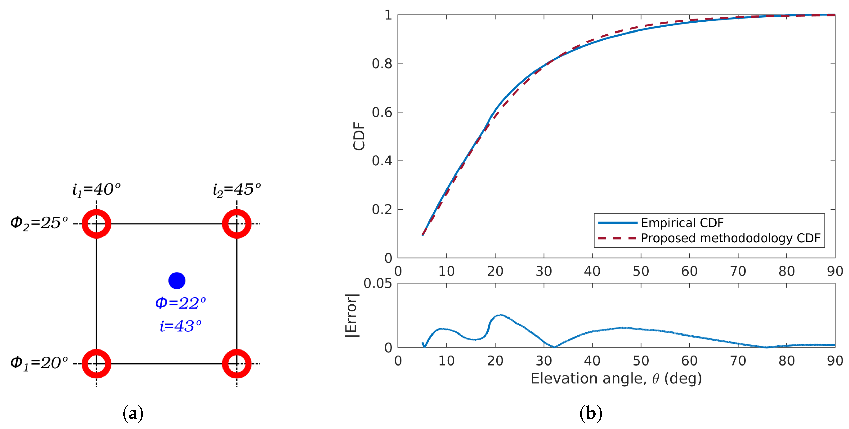
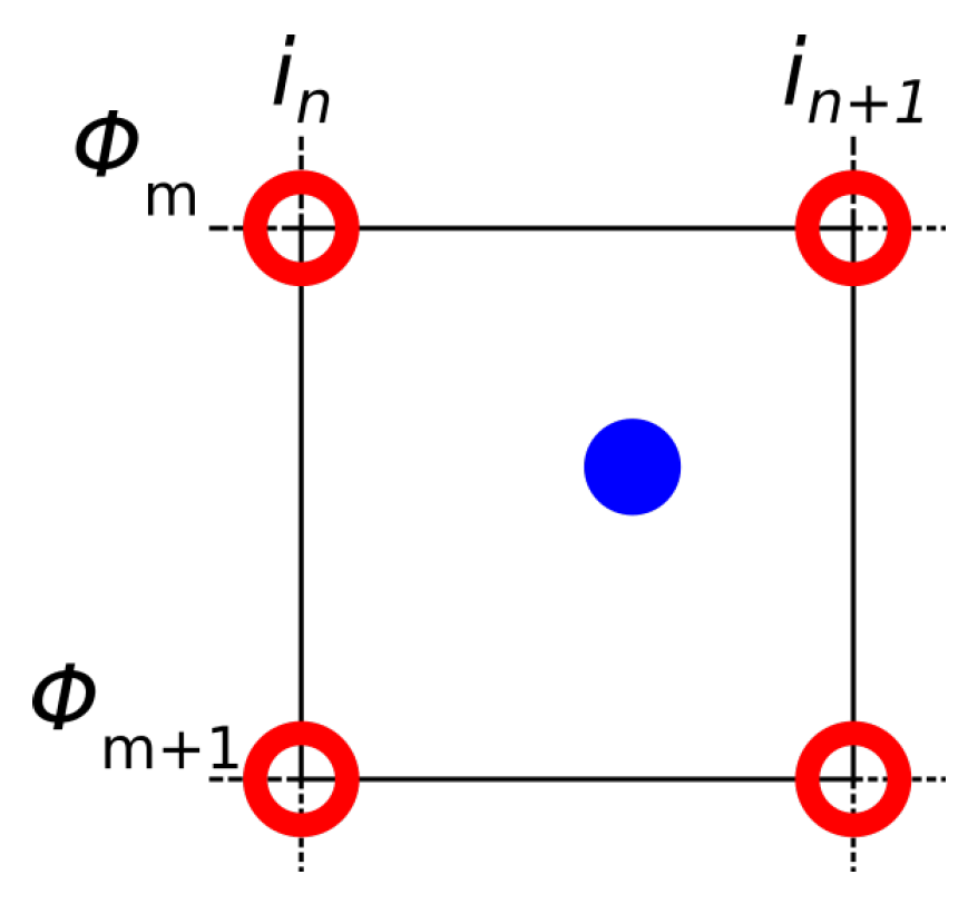
Interpolation for a Four-Point Mesh

The bilinear method is proposed as the method to find the query point inside the mesh since it is a well-known method and widely applied for interpolation.
We can obtain the values for a query point as in Figure A2 for a shape parameter value a using bilinear interpolation as follows
a ( ϕ , i ) = w 1 a ( ϕ 2 , i 1 ) + w 2 a ( ϕ 1 , i 1 ) + w 3 a ( ϕ 2 , i 2 ) + w 4 a ( ϕ 1 , i 2 ) ,
similarly, we can obtain the scale parameter, b, using bilinear interpolation as follows
b ( ϕ , i ) = w 1 b ( ϕ 2 , i 1 ) + w 2 b ( ϕ 1 , i 1 ) + w 3 b ( ϕ 2 , i 2 ) + w 4 b ( ϕ 1 , i 2 ) ,
where the wights w 1 , w 2 , w 3 and w 4 are given by
w 1 = ( i 2 i ) ( ϕ 1 ϕ ) / [ ( i 2 i 1 ) ( ϕ 1 ϕ 2 ) ]
w 2 = ( i 2 i ) ( ϕ ϕ 2 ) / [ ( i 2 i 1 ) ( ϕ 1 ϕ 2 ) ]
w 3 = ( i i 1 ) ( ϕ 1 ϕ ) / [ ( i 2 i 1 ) ( ϕ 1 ϕ 2 ) ]
w 4 = ( i i 1 ) ( ϕ 1 ϕ 2 ) / [ ( i 2 i 1 ) ( ϕ 1 ϕ 2 ) ]
where the known values for a ( i n , ϕ m ) , , a ( i n + 1 , ϕ m + 1 ) and b ( i n , ϕ m ) , , b ( i n + 1 , ϕ m + 1 ) , can be obtained from matrices A h and B h .
Figure A2. F θ ( Θ ) for two orbit configurations.
Applsci 13 04405 g0a2

References

  1. Crowe, K.; Raines, R. A model to describe the distribution of transmission path elevation angles to the Iridium and Globalstar satellite systems. IEEE Commun. Lett. 1999, 3, 242–244. [Google Scholar] [CrossRef] [Green Version]
  2. Li, S.Y.; Liu, C. An analytical model to predict the probability density function of elevation angles for LEO satellite systems. IEEE Commun. Lett. 2002, 6, 138–140. [Google Scholar] [CrossRef]
  3. Corazza, G.; Vatalaro, F. A statistical model for land mobile satellite channels and its application to nongeostationary orbit systems. IEEE Trans. Veh. Technol. 1994, 43, 738–742. [Google Scholar] [CrossRef]
  4. Davoli, F.; Kourogiorgas, C.; Marchese, M.; Panagopoulos, A.; Patrone, F. Small satellites and CubeSats: Survey of structures, architectures, and protocols. Int. J. Satell. Commun. Netw. 2019, 37, 343–359. [Google Scholar] [CrossRef]
  5. del Portillo, I.; Cameron, B.G.; Crawley, E.F. A technical comparison of three low earth orbit satellite constellation systems to provide global broadband. Acta Astronaut. 2019, 159, 123–135. [Google Scholar] [CrossRef]
  6. Popescu, O. Power Budgets for CubeSat Radios to Support Ground Communications and Inter-Satellite Links. IEEE Access 2017, 5, 12618–12625. [Google Scholar] [CrossRef]
  7. Hu, J.; Li, G.; Bian, D.; Gou, L.; Wang, C. Optimal Power Control for Cognitive LEO Constellation With Terrestrial Networks. IEEE Commun. Lett. 2020, 24, 622–625. [Google Scholar] [CrossRef]
  8. Chobotov, V.A. Orbital Mechanics, 3rd ed.; AIAA: Reston, VA, USA, 2002. [Google Scholar]
  9. Gongora-Torres, J.M.; Vargas-Rosales, C.; Aragón-Zavala, A.; Villalpando-Hernandez, R. Link Budget Analysis for LEO Satellites Based on the Statistics of the Elevation Angle. IEEE Access 2022, 10, 14518–14528. [Google Scholar] [CrossRef]
  10. Kolawole, M.O. Satellite Communication Engineering; Marcel Dekker, Inc.: New York, NY, USA, 2002; Chapter 2. [Google Scholar]
  11. Zhengsheng, C.; Qinghua, Z.; Xuerui, L.; Dashuang, S.; Hao, L.; Runtao, Z.; Jinlong, C. A reference satellite selection method based on maximal elevation angle during the observation period. In Proceedings of the 2017 Forum on Cooperative Positioning and Service, CPGPS 2017, 2017, number 2017 Forum on Cooperative Positioning and Service, CPGPS 2017, Harbin, China, 19–21 May 2017; pp. 268–272. [Google Scholar]
  12. Seyedi, Y. A Trace-Time Framework for Prediction of Elevation Angle Over Land Mobile LEO Satellites Networks. Wirel. Pers. Commun. 2012, 62, 793–804. [Google Scholar] [CrossRef]
  13. Su, Y.; Liu, Y.; Zhou, Y.; Yuan, J.; Cao, H.; Shi, J. Broadband LEO Satellite Communications: Architectures and Key Technologies. IEEE Wirel. Commun. 2019, 26, 55–61. [Google Scholar] [CrossRef]
  14. Qu, Z.; Zhang, G.; Cao, H.; Xie, J. LEO Satellite Constellation for Internet of Things. IEEE Access 2017, 5, 18391–18401. [Google Scholar] [CrossRef]
  15. Lopez-Salamanca, J.J.; Seman, L.O.; Berejuck, M.D.; Bezerra, E.A. Finite-State Markov Chains Channel Model for CubeSats Communication Uplink. IEEE Trans. Aerosp. Electron. Syst. 2020, 56, 142–154. [Google Scholar] [CrossRef]
  16. Tropea, M.; De Rango, F. A Comprehensive Review of Channel Modeling for Land Mobile Satellite Communications. Electronics 2022, 11, 820. [Google Scholar] [CrossRef]
  17. Saeed, N.; Elzanaty, A.; Almorad, H.; Dahrouj, H.; Al-Naffouri, T.Y.; Alouini, M.S. CubeSat Communications: Recent Advances and Future Challenges. IEEE Commun. Surv. Tutor. 2020, 22, 1839–1862. [Google Scholar] [CrossRef]
  18. Kodheli, O.; Lagunas, E.; Maturo, N.; Sharma, S.K.; Shankar, B.; Montoya, J.F.M.; Duncan, J.C.M.; Spano, D.; Chatzinotas, S.; Kisseleff, S.; et al. Satellite Communications in the New Space Era: A Survey and Future Challenges. IEEE Commun. Surv. Tutor. 2021, 23, 70–109. [Google Scholar] [CrossRef]
  19. Arapoglou, P.D.; Liolis, K.; Bertinelli, M.; Panagopoulos, A.; Cottis, P.; De Gaudenzi, R. MIMO over Satellite: A Review. IEEE Commun. Surv. Tutor. 2011, 13, 27–51. [Google Scholar] [CrossRef]
  20. Baeza, V.M.; Lagunas, E.; Al-Hraishawi, H.; Chatzinotas, S. An Overview of Channel Models for NGSO Satellites. In Proceedings of the 2022 IEEE 96th Vehicular Technology Conference (VTC2022-Fall), London, UK, 26–29 September 2022; pp. 1–6. [Google Scholar] [CrossRef]
  21. Loo, C. A statistical model for a land mobile satellite link. IEEE Trans. Veh. Technol. 1985, 34, 122–127. [Google Scholar] [CrossRef]
  22. Lutz, E.; Cygan, D.; Dippold, M.; Dolainsky, F.; Papke, W. The Land Mobile Satellite Communication Channel-Recording, Statistics, and Channel Model. IEEE Trans. Veh. Technol. 1991, 40, 375–386. [Google Scholar] [CrossRef]
  23. Abdi, A.; Lau, W.C.; Alouini, M.S.; Kaveh, M. A new simple model for land mobile satellite channels: First- and second-order statistics. IEEE Trans. Wirel. Commun. 2003, 2, 519–528. [Google Scholar] [CrossRef] [Green Version]
  24. Fontan, F.; Vazquez-Castro, M.; Cabado, C.; Garcia, J.; Kubista, E. Statistical modeling of the LMS channel. IEEE Trans. Veh. Technol. 2001, 50, 1549–1567. [Google Scholar] [CrossRef]
  25. National Aeronautics and Space Administration. General Mission Analysis Tool (GMAT) Version R2022a. Available online: http://sourceforge.net/projects/gmat/ (accessed on 15 March 2022).
  26. Gongora-Torres, J.M. Time Series for LEO. Available online: https://figshare.com/articles/dataset/TimeSeries_zip/22292953 (accessed on 17 March 2022).
  27. Al-Hraishawi, H.; Chougrani, H.; Kisseleff, S.; Lagunas, E.; Chatzinotas, S. A Survey on Nongeostationary Satellite Systems: The Communication Perspective. IEEE Commun. Surv. Tutor. 2022, 25, 101–132. [Google Scholar] [CrossRef]
  28. Papoulis, A. Probability, Random Variables, and Stochastic Processes; McGraw-Hill: New York, NY, USA, 1984. [Google Scholar] [CrossRef]
Figure 1. Elevation angle cases for LEO satellite systems: (a) The values of θ m i n and θ m a x are usually related to the best and worst case of the received power, P R , at an ES; nonetheless, those cases are rare and represent the extremes of θ . (b) The elevation angle of a LEO satellite system as observed from an ES is always-varying; then, it is more convenient to analyze its behavior through statistical tools.
Applsci 13 04405 g001
Figure 2. Basic structure and contents of this article.
Applsci 13 04405 g002
Figure 3. LEO characteristics: (a) Graphical representation of the always-varying elevation angle, θ , and (b) an On-Off model showing the link availability for a LEO satellite vs a GEO satellite during a random day.
Applsci 13 04405 g003
Figure 4. First order Markov chain illustrating the channel model developed by Lutz [22].
Applsci 13 04405 g004
Figure 5. Generalization of a three-state channel model as proposed by [24] considering state transitions based on elevation angle changes.
Applsci 13 04405 g005
Figure 6. Loo CDF of the received signal for two elevation angle values. The Loo triplet for θ 1 = 10 ° is α = −105 dB, ψ = 5 dB, and M P = −108 dB; and α = −95 dB, ψ = 5 dB, and M P = −98 dB for θ 2 = 90 ° .
Applsci 13 04405 g006
Figure 7. (a) Histogram and (b) theoretical densities for one of the elevation angle data sets obtained from the performed simulations.
Applsci 13 04405 g007
Figure 8. Kolmogorov-Smirnov statistic for the performed simulations at different altitudes.
Applsci 13 04405 g008
Figure 9. Simulated orbits: (a) Model without scale illustrating satellite passes at different orbit inclinations, i, over different ES’s latitudes. (b) Simulated orbit inclinations and ES’s latitudes as points in a grid. (c) Reduction of the grid showing in each column the ES’s below the simulated orbit inclinations. (d) Simulated points as diagonal elements within a matrix.
Applsci 13 04405 g009
Figure 10. Comparison and error of the empirical and Gamma elevation angle CDF’s for different ES latitudes, ϕ E S , orbit inclinations of the satellites, i S A T , and, orbit altitudes, h k . (a) CDF’s for ϕ E S = 30 ° and i S A T = 30 ° at h k = 1000 km; (b) CDF’s for ϕ E S = 45 ° and i S A T = 65 ° at h k = 1000 km; (c) CDF’s for ϕ E S = 20 ° and i S A T = 75 ° at h k = 1000 km; (d) CDF’s for ϕ E S = 85 ° and i S A T = 85 ° at h k = 1000 km.
Applsci 13 04405 g010
Figure 11. Example case results for ϕ E S = 22 ° , i S A T = 43 ° and h k = 1500 km: (a) four-point mesh to calculate the shape, a, and scale, b parameters of f θ ( θ ) and (b) empirical CDF vs. CDF obtained with the proposed methodology.
Applsci 13 04405 g011
Figure 12. PDF and CDF for two orbit configurations sharing the same altitude, eccentricity, and orbit inclination, but with the remaining orbital parameters being different.
Applsci 13 04405 g012
Figure 13. CDF F Θ ( θ ) for the same orbit configuration and ES latitude but for (a) different ES longitude and (b) different simulation period.
Applsci 13 04405 g013
Figure 14. CDF F Θ ( θ ) for different satellite mass and drag area characteristics.
Applsci 13 04405 g014
Figure 15. CDF’s for the absolute errors at different orbit configurations and ES’s as in Figure 10a–d. Absolute error CDF’s for: (a) ϕ E S = 30 ° and i S A T = 30 ° at h k = 1000 km; (b) ϕ E S = 45 ° and i S A T = 65 ° at h k = 1000 km; (c) ϕ E S = 20 ° and i S A T = 75 ° at h k = 1000 km; (d) ϕ E S = 85 ° and i S A T = 85 ° at h k = 1000 km.
Applsci 13 04405 g015
Figure 16. Distribution of the absolute errors behavior of all the performed simulations: (a) PDF, (b) CDF, and (c) CCDF.
Applsci 13 04405 g016
Figure 17. CDF’s of the absolute error by elevation angle range for all the simulated orbits and ES’s.
Applsci 13 04405 g017
Figure 18. Boxplots of the absolute error by elevation angle range. Simulation results vs proposed methodology.
Applsci 13 04405 g018
Table 1. Satellite characteristics for the ephemeris generation.
Dry MassDrag AreaSolar Radiation Pressure Area
5 kg1 m 2 1 m 2
Table 2. Orbit characteristics for the ephemeris generation.
Semi-Major Axis, aOrbit Inclinations, i
17378 km20 ° , 25 ° , , 85 °
27578 km20 ° , 25 ° , , 85 °
37778 km20 ° , 25 ° , , 85 °
47978 km20 ° , 25 ° , , 85 °
58178 km20 ° , 25 ° , , 85 °
68378 km20 ° , 25 ° , , 85 °
Table 3. ES locations for the performed simulations specified through their latitude, ϕ , and longitude, λ .
LatitudeLongitude LatitudeLongitude
ES 1 0 ° 276.7121 ° ES 10 45 ° 259.7121 °
ES 2 5 ° 276.7121 ° ES 11 50 ° 259.7121 °
ES 3 10 ° 276.7121 ° ES 12 55 ° 259.7121 °
ES 4 15 ° 267.7121 ° ES 13 60 ° 259.7121 °
ES 5 20 ° 276.7121 ° ES 14 65 ° 259.7121 °
ES 6 25 ° 261.7121 ° ES 15 70 ° 265.7121 °
ES 7 30 ° 259.7121 ° ES 16 75 ° 265.7121 °
ES 8 35 ° 259.7121 ° ES 17 80 ° 265.7121 °
ES 9 40 ° 259.7121 ° ES 18 −85 ° 259.7121 °
Table 4. Rate parameter, a, of the gamma distribution to characterize the elevation angle distribution at ES 1 , for different altitudes, h, and orbit inclinations, i.
ES 1 20 ° 25 ° 30 ° 35 ° 40 ° 45 ° 50 ° 55 ° 60 ° 65 ° 70 ° 75 ° 80 ° 85 °
7378 km1.391.501.481.311.301.341.351.351.351.371.371.361.361.37
7578 km1.621.791.801.651.561.611.621.631.631.641.641.641.641.64
7778 km1.571.771.821.731.551.611.631.641.641.651.651.661.661.66
7978 km1.631.741.831.791.621.601.631.651.651.661.661.661.661.67
8178 km1.701.661.831.821.701.551.631.651.661.671.671.671.701.67
8378 km1.751.671.821.841.751.581.631.661.671.681.681.681.681.68
Table 5. Scale parameter of the gamma distribution, b × 10 2 , to characterize the elevation angle distribution at ES 1 , for different altitudes, h, and orbit inclinations, i.
ES 1 20 ° 25 ° 30 ° 35 ° 40 ° 45 ° 50 ° 55 ° 60 ° 65 ° 70 ° 75 ° 80 ° 85 °
7378 km7.518.719.348.888.408.428.408.368.348.398.388.358.358.36
7578 km7.869.139.919.749.059.028.998.978.938.958.948.938.918.91
7778 km7.458.559.419.568.838.738.708.678.648.668.648.648.638.64
7978 km7.418.088.989.338.888.488.468.448.408.418.398.398.388.39
8178 km7.387.598.609.078.888.188.268.248.228.228.208.188.268.18
8378 km7.347.478.278.828.838.218.098.088.068.058.038.028.008.02
Table 6. Shape parameter, a, for matrix P a , using the diagonal notation as in (19), and as shown in Figure 9d.
Diagonals Range
Altitude( d 4 , d 2 )( d 1 , d 0 )( d 1 , d 2 )( d 3 , d 13 )
1000 km1.4709541.6384251.4507941.488802
1200 km1.7073231.9353211.7215721.752709
1400 km1.7129231.9515201.7462051.754760
1600 km1.7234361.9552541.7821901.757023
1800 km1.7311101.9523621.7965491.774827
2000 km1.7414501.9547941.8368331.760709
Table 7. Rate parameter, b × 10 2 , for matrix P b , using the diagonal notation as in (19), and as shown in Figure 9d.
Diagonals Range
Altitude( d 4 , d 2 )( d 1 , d 0 )( d 1 , d 2 )( d 3 , d 13 )
1000 km7.0370529.4594599.0758058.805617
1200 km7.3919639.8400109.6404369.284945
1400 km7.1305879.3194369.4124128.952740
1600 km6.9439988.8794569.2421468.693598
1800 km6.7910488.5105889.0416048.632867
2000 km6.6751828.2245038.9414248.305444
Table 8. First and second order statistics of the elevation angle for the same orbit configurations and ES’s locations that in Figure 10a–d.
Empirical ResultProposed Method’s ResultEmpirical ResultProposed Method’s ResultsEmpirical ResultProposed Method’s ResultsEmpirical ResultProposed Method’s Results
ES latitude, ϕ E S 30 ° 45 ° 20 ° 85 °
Orbit inclination, i S A T 30 ° 65 ° 75 ° 85 °
Orbit altitude, h S A T 1000 km
Shape parameter, a1.47101.63841.48881.8387
Rate Parameter, b × 10 2 7.03719.45958.80567.0371
E [ Θ > 5 ° ] 24.55 ° 23.09 ° 19.43 ° 19.74 ° 20.24 ° 19.70 ° 27.70 ° 26.66 °
SD [ Θ > 5 ° ] 18.40 ° 16.86 ° 14.19 ° 13.13 ° 14.94 ° 13.48 ° 18.12 ° 18.90 °
E [ Θ > 15 ° ] 34.77 ° 31.13 ° 29.77 ° 27.96 ° 30.55 ° 28.24 ° 35.48 ° 33.23 °
SD [ Θ > 15 ° ] 17.46 ° 16.26 ° 14.24 ° 12.45 ° 14.49 ° 12.93 ° 16.32 ° 17.96 °
E [ Θ > 25 ° ] 44.33 ° 39.66 ° 40.12 ° 37.03 ° 40.39 ° 37.38 ° 42.73 ° 40.91 °
SD [ Θ > 25 ° ] 15.93 ° 15.88 ° 13.40 ° 12.05 ° 13.50 ° 12.61 ° 14.79 ° 17.29 °
Table 9. Shape and scale parameters for the elevation angle PDF and CDF for ϕ E S = 22 ° and i S A T = 43 ° at h k = 1500 km, corresponding to the four-point mesh shown in Figure 11a.
Four-Point Mesh Setup
14001600 14001600
a ( ϕ 1 , i 1 ) 1.95151.9552 b ( ϕ 1 , i 1 ) 9.3194 × 10 2 8.8794 × 10 2
a ( ϕ 1 , i 2 ) 1.95151.9552 b ( ϕ 1 , i 2 ) 9.3194 × 10 2 8.8794 × 10 2
a ( ϕ 2 , i 1 ) 1.95151.9552 b ( ϕ 2 , i 1 ) 9.3194 × 10 2 8.8794 × 10 2
a ( ϕ 2 , i 2 ) 1.74621.7822 b ( ϕ 2 , i 2 ) 9.4112 × 10 2 9.2215 × 10 2
Obtained parameters from interpolation
a ( ϕ , i ) 1.87761.8929 b ( ϕ , i ) 9.3529 × 10 2 9.0025 × 10 2
a ( ϕ , i ) 1.8853 b ( ϕ , i ) 9.1777 × 10 2
Empirical parameters
a ( ϕ , i ) 1.9804 b ( ϕ , i ) 9.5987 × 10 2
Table 10. Satellites with different mass and drag area characteristics for additional performed simulations.
Satellite 1Satellite 2
Dry mass5 kg200 kg
Drag area1 m 2 10 m 2
Solar radiation pressure area1 m 2 10 m 2
Disclaimer/Publisher’s Note: The statements, opinions and data contained in all publications are solely those of the individual author(s) and contributor(s) and not of MDPI and/or the editor(s). MDPI and/or the editor(s) disclaim responsibility for any injury to people or property resulting from any ideas, methods, instructions or products referred to in the content.

