
Free Vibration of Rectangular Composite Cantilever Plate and Its Application in Material Degradation Assessment

Department of Mechanical Engineering, National Yang Ming Chiao Tung University, Hsinchu 30010, Taiwan
*
Author to whom correspondence should be addressed.
Appl. Sci. 2023, 13(8), 5101; https://0-doi-org.brum.beds.ac.uk/10.3390/app13085101
Submission received: 17 March 2023
/
Revised: 10 April 2023
/
Accepted: 14 April 2023
/
Published: 19 April 2023
(This article belongs to the Special Issue Structural Vibration: Analysis, Control, Experiment, and Applications II)
Abstract
:Many composite cantilever plate-like structures have found engineering applications in different industries. For attaining a meaningful assessment of the plate vibration characteristics, it is important to have efficient and effective methods for determining the natural frequencies/mode shapes of composite cantilever plates. In this paper, a method formulated on the basis of the Ritz method and a simple first-order shear deformation theory (SFSDT) is presented to analyze the free vibration of thin as well as thick rectangular composite cantilever plates for determining their natural frequencies. In the SFSDT, the total deflection is the sum of two deflection components, namely, bending and through-thickness shear-deformation-induced deflections. The successful application of the Ritz method together with the SFSDT for the free vibration analysis of thick composite plates relies on the selection of two independent sets of characteristic functions for the bending and through-thickness shear-deformation-induced deflections, respectively, to satisfy the requirements for the displacement and force conditions at the fixed edge of the plate. The novelty of the proposed method is that two independent sets of characteristic functions, namely, polynomials and trigonometric functions, which satisfy the displacement and force conditions at the fixed edge have been identified and used in the variational method to construct the eigenvalue problem for extracting the modal characteristics (natural frequencies and mode shapes) of the plate. It has been shown that the uses of the selected characteristic functions can produce excellent natural frequencies for both thin and thick composite cantilever plates. Some existing theoretical and experimental natural frequencies of thin as well as thick composite plates have been used to demonstrate the accuracy of the proposed method in predicting natural frequencies. The significant effects of through-thickness shear deformation on the natural frequencies of composite cantilever plates are studied to show the merit of the present method. Finally, for illustrating the application of the proposed method in free vibration analysis, a novel procedure established on the basis of the sensitivity analysis of natural frequencies is presented to assess the material degradation of composite cantilever plates. The numerical examples have shown that fewer than 10 iterations are required in the identification process to produce a good estimation of the current value for each material constant.
1. Introduction
Modal characteristics (natural frequency and mode shape) have found different applications in the areas of structural engineering and solid mechanics. For instance, for safety reasons, modal characteristics are important parameters to be dealt with in the design, system identification, and health monitoring of a structure. Regarding the design of a structure subject to dynamic loads, the natural frequencies of the structure must be taken into consideration to prevent resonance from occurring. Therefore, to avoid the occurrence of resonance, many papers have been devoted to the optimal design of structures with the consideration of natural frequency constraints [1,2,3,4,5]. Regarding health monitoring/assessment, the modal characteristics of a damaged structure are important information for assessing structural damage. For instance, many papers have been devoted to the use of natural frequencies/mode shapes for detecting damage in structures [6,7,8,9,10,11,12]. In the area of system identification, many researchers have used natural frequencies/mode shapes to identify the system parameters of composite structures [13,14,15,16,17,18,19,20]. For instance, Lee and Kam [17] used natural frequencies in a Ritz-based method to identify the material constants of flexibly restrained plates. In the acoustic area, modal characteristics information has been used to modify the vibration behavior of flat-panel sound radiators for enhancing their sound radiation efficiency [21,22,23]. For instance, Jiang et al. [23] used the information of modal characteristics to mitigate sound pressure level dips for smoothing the sound pressure level curves of composite panel-form speakers. Therefore, the above literature review has shown that modal characteristics are important structural parameters that have found many different engineering applications. Cantilever-plate/beam-like structural parts such as turbine blades, fighter spoilers, aircraft stabilizers, and missile fins are subject to dynamic loads which can cause them to vibrate. Furthermore, because of their importance, many research papers have been published to focus on the free vibration analysis of cantilever-plate/beam-like structural parts and different methods have been proposed to determine their modal characteristics [24,25,26,27,28,29,30,31,32,33,34,35,36,37]. Therefore, from the engineering application point of view, it is still desirable to develop more efficient and effective methods for predicting the actual vibration behavior of these types of structures. On the other hand, advanced composite materials have many attractive properties such as high strength in the fiber direction, ease of being tailored to make fibers coincide with the direction of stress flow, light weight, and super corrosion resistance capability. Recently, they have been used to fabricate vibration-susceptible composite plate structures in the wind power, aerospace, aircraft, and defense industries, among others. The wide application of composite plates in different industries has led to the development of different methods for determining the modal characteristics of composite plates [38,39,40,41,42,43,44,45,46,47,48,49]. In particular, due to its simplicity of implementation, effectiveness in producing reliable results, and computational efficiency, the Ritz method has been widely used for the free vibration analysis of plates. For instance, Kam et al. [46] used Legendre polynomials as characteristic functions in the Ritz method to study the free vibration and sound radiation of elastically restrained shear deformable stiffened composite plates. Regarding the use of the Ritz method in vibration analysis, it is noted that the appropriateness of the chosen characteristic functions can have significant effects on the accuracy of the modal characteristics. When the thickness of a plate increases, the effects of through-thickness shear deformation on the plate deflection may become too significant to be neglected. However, in the previous studies, cantilever-type composite plate structures were treated as thin plates and the classical lamination theory (CLT) was used to analyze the free vibration of such plates. The CLT does not consider the through-thickness shear deformation so it is only suitable for the analysis of thin plates. In fact, the thicknesses of many cantilever-type plate structures used in different industries are generally relatively large so the classical lamination theory becomes inappropriate for modeling the vibration behavior of such plate structures. Therefore, in order to have more realistic predictions of the vibration characteristics of relatively thick cantilever-type composite plate structures, there is a need to develop an appropriate method that can take the through-thickness shear deformation into consideration. Recently, detailed reviews on different shear deformation theories for modeling composite plate deflection have been conducted [50,51]. Among the shear deformation theories, the commonly used theory for plate analysis is the conventional first-order shear deformation theory (FSDT) [52,53]. In the conventional FSDT, five independent displacement components (three displacement components at the mid-plane and two shear rotations) are required to describe the displacement field of a thick plate. Furthermore, shear correction factors are needed to correct the effects of uniform shear stress distribution over the plate thickness on the strain energy of the plate. Several methods studying the calculation of shear correction factors for composite laminates have been reported in the literature [54,55,56,57,58]. Besides the conventional FSDT, another type of FSDT, which is termed simple first-order shear deformation theory (SFSDT), has been used for engineering applications. Contrary to the conventional FSDT, the simple first-order shear deformation theory (SFSDT) only uses four displacement components to describe the displacement field of a composite plate. Hence, with respect to computational efficiency, the SFSDT seems to be more advantageous than the conventional FSDT. Recently, a number of researchers have attempted to apply SFSDT to plate analysis [59,60,61,62,63,64,65]. For instance, Thai and his associates [59,60,61] used SFSDT-based methods to analyze various functionally graded/laminated composite/sandwich plates and beams with different boundary and loading conditions. In their studies, they adopted a shear correction factor of 5/6 to analyze very thick plates with a length-to-thickness ratio (a/h) as small as 2 in the numerical examples for illustration. Senjanović [62] developed an SFSDT-based finite element method to analyze thick plates with a/h ≥ 5 using a shear correction factor equal to 5/6 or 0.8667. Park and Choi [65] applied the SFSDT to study the bending, buckling, and free vibration of isotropic plates with the consideration of the in-plane rotation and the use of a shear correction factor of 5/6. In applying the SFSDT, some researchers have introduced warping functions to approximate the deformed shapes of the plane cross-sections after deformation and satisfy the shear stress boundary conditions on the top and bottom plate surfaces [66,67,68,69,70]. It is noted that all the above works formulated on the basis of SFSDT have derived the governing equations or equations of motion for plate analysis. The use of the above SFSDT-based methods for free vibration analysis of thick cantilever composite plates may be computationally expensive or not simple enough for engineering applications. By contrast, the incorporation of the advantages of the Ritz method and the SFSDT may produce a useful technique for plate analysis. Hence, it is worth putting effort into developing the method formulated on the basis of the Ritz method and SFSDT for the vibration analysis of composite cantilever plates with the consideration of engineering applications. On the other hand, it is desirable to have an efficient and effective tool for determining the modal characteristics of thick composite cantilever plates for solving engineering problems such as resonance mitigation, material constants identification, and damage detection. For instance, the natural frequencies of composite cantilever plates can be used to characterize the material properties of the plates. In particular, the identification of the current material constants for a plate can help assess the material degradation/structural health of the plate. As mentioned above, many methods have been proposed to identify the material constants of composite plates from natural frequencies. In general, most of the existing material constant identification methods have attempted to determine all the material constants at the same time. However, when the number of the material constants increases, many of the existing methods may face one or both of the two difficulties, i.e., it is difficult to make the solution converge and computationally expensive. For practical applications, many methods may not be efficient enough to be used in material degradation assessment. Therefore, regarding practical applications, it is still desirable to search for more efficient and effective methods for material degradation assessment. Hence, the incorporation of the proposed SFSDT-based Ritz method and a useful procedure for material degradation assessment of composite cantilever plates using natural frequencies is the aim of this paper.
In this paper, a new SFSDT-based Ritz method is presented to study the free vibration of composite cantilever plates with different length-to-thickness ratios. Appropriate characteristic functions are proposed to approximate the deflection components which lead to the total deflection of the plate. The theoretical and experimental natural frequencies obtained using different methods are used to verify the accuracy of the proposed method. The effects of plate thickness and fiber angles on the natural frequencies and mode shapes of composite cantilever plates are studied by means of several numerical examples. A novel procedure with the consideration of the information obtained from the sensitivity analysis of natural frequency is presented for material degradation assessment. The proposed procedure is able to produce a good estimation of any material constant in a few iterations in the identification process. The material degradation assessment of composite cantilever plates is performed to show one of the applications of the proposed method.
2. Vibration Analysis of Composite Cantilever Plate
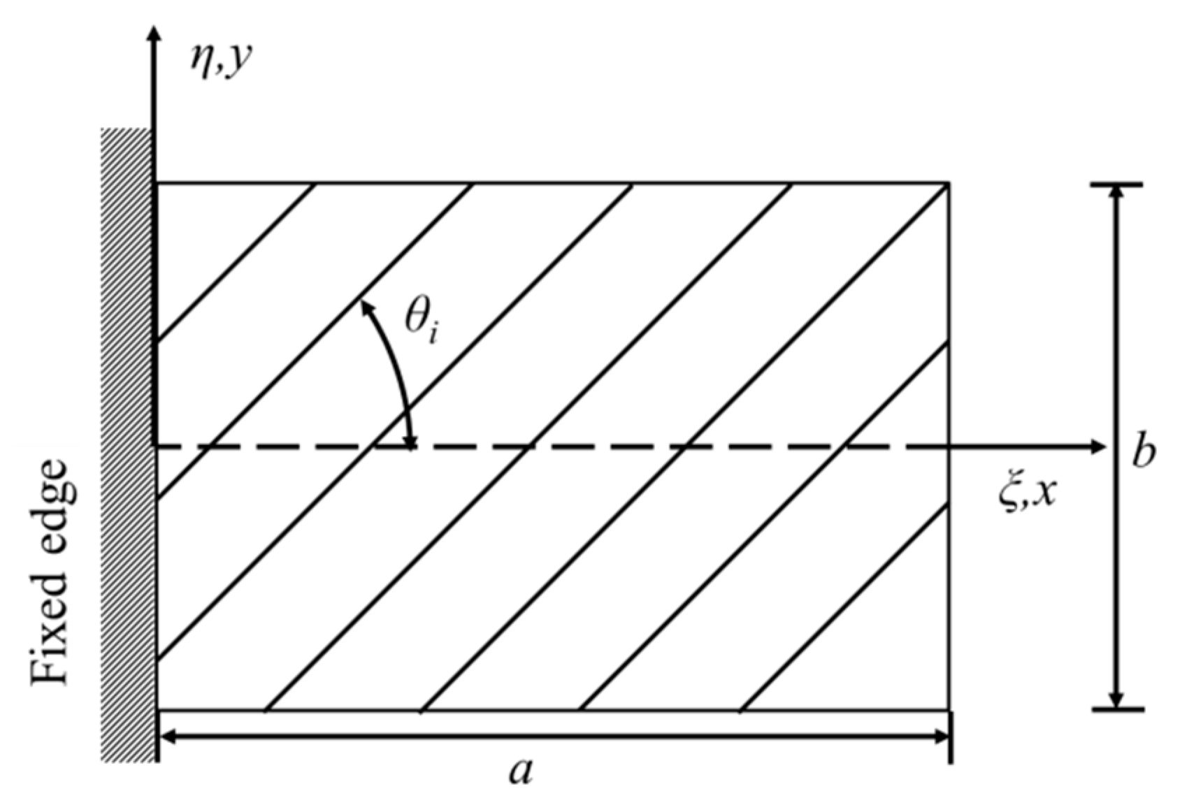
Consider the free vibration of a rectangular symmetrically laminated composite plate of size a (length) × b (width) × h (thickness) with the left end clamped as shown in Figure 1. The fiber angle of the ith layer is θi. Herein, two coordinate systems, namely, reference coordinate system x-y-z and natural coordinate system ξ-η-z are used to describe the geometry of the plate. Both x-y and ξ-η are located at the mid-plane of the plate with (0 ≤ x ≤ a, −b/2 ≤ y ≤ b/2) and (0 ≤ ξ ≤ 1, −0.5 ≤ η ≤ 0.5), respectively. The relation between the two coordinate systems is ξ = x/a and η = y/b.
In the SFSDT, the total vertical deflection is the sum of two parts, namely, the bending and through-thickness shear-deformation-induced deflections. Assuming no plate thickness change and neglecting the in-plane displacements, the displacement field of the symmetrically laminated plate under free vibration is written as
where u, v, and w are the displacement components in the x-y-z coordinate system of the plate; wb is the vertical deflection induced by bending; and ws is the vertical deflection induced by through-thickness shear deformation. It is noted that herein only two independent displacement components (wb and ws) rather than three independent displacement components (two shear rotations plus one vertical deflection) for the FSDT are required to describe the displacement field of the plate. In general, it is common practice to use the natural coordinate system to express the characteristic functions in the Ritz method. Hence, in the free vibration analysis, the vertical displacement components of the plate in the ξ-η coordinate system are expressed as
where Wb and Ws are the bending and through-thickness shear-deformation-induced deflected shapes, respectively. Referring to the ξ-η coordinate system, discarding the effect of time, the strain-displacement relations of the plate are expressed as
where ε and γ are the normal and shear strains, respectively. The stress–strain relations of a composite lamina with arbitrary fiber angle in the ξ-η-z coordinate system can be expressed in the following general form [71]:
where σ and τ are the normal and shear stresses, respectively, and is the transformed lamina stiffness coefficient, which depends on the material properties and lamina fiber angle. The relations between the transformed and untransformed lamina stiffness coefficients are expressed as
with
where Qij is the untransformed lamina stiffness constant, Ei is Young’s modulus in the ith direction, νij is Poisson’s ratio, and Gij is the in-plane shear modulus. For simplicity, the stress–strain relations in Equation (4) for the ith layer in the plate can be written in matrix form as
The strain energy U of the plate can be expressed as
In view of Equations (1), (4), and (8), the maximum strain energy Umax of the plate can be expressed as
or
with
and
where α = b/a, Kp = shear correction factor, and NL = number of layers. Regarding the determination of Kp, as mentioned above, the exact values of Kp for different composite laminates can be calculated using the methods reported in the literature. In fact, for engineering applications, a database collecting the exact values of Kp for different composite laminates can be established. Herein, for illustration purposes and also without loss of generality, Kp is assumed to be 0.8. With the consideration of the rotatory inertia effects, the kinetic energy T of the plate with density ρ and the inclusion of rotatory effects is expressed as
In view of Equations (2) and (13), the maximum kinetic energy Tmax can be written as
The Lagrangian to be used in the Ritz method for the plate is defined as
According to the Ritz method, each plate displacement can be approximated using a finite series of characteristic functions associated with equal numbers of unknown constants. If the approximated displacements are substituted into Equation (15), the Lagrangian L will be a function of the undetermined constants. The extremization of L with respect to the undetermined constants leads to the following eigenvalue problem:
where K is the stiffness matrix, M, the mass matrix, and C a vector of the undetermined constants. The solution to the above eigenvalue problem can lead to the determination of the natural frequencies and mode shapes of the plate.
3. Ritz Method
Regarding the use of the Ritz method in the above plate vibration analysis, it is noted that the choice of appropriate characteristic functions for approximating the bending and through-thickness shear-deformation-induced vertical deflection components is vital in attaining good approximations of the true modal characteristics of the plate. Two issues should be dealt with in determining the characteristic functions. The first issue is related to the independence between the two sets of characteristic functions for Wb and Ws, respectively. In view of the total deflection in Equation (1), the two sets of characteristic functions must be independent so that each deflection component can have its own contribution to the total deflection. It is worth noting that if the two sets of characteristic functions are dependent, then, after summation, only one set of characteristic functions will be left to approximate the total deflection. The consequence of the choice of dependent sets of characteristic functions is that the contribution of Ws to the total deflection will be underestimated. It has been found that the underestimation of the total deflection will lead to incorrect predictions of natural frequencies for thick plates, especially those with a/h less than 50. The second issue is related to the satisfaction of the displacement and force conditions at the fixed edge of the cantilever plate. In view of the displacement boundary conditions at the fixed edge of the cantilever plate, it is required that the vertical displacement and bending rotation at ξ = 0 equal to zero
In view of Equation (1), Equation (17) can be rewritten as
and
As indicted in Ref. [72], different displacement boundary conditions at the fixed end of a cantilever beam can be chosen to solve for the deflection of the beam under the conditions that the bending moment and shear force at the fixed end are not zero. For the cantilever plate under consideration in this study, the requirements of nonzero bending moment and shear force at the fixed edge of the plate must be observed to maintain the equilibrium/stability of the plate. It is noted that in view of Equation (3), for having nonzero shear strain/shear stress at the fixed edge of the plate, should not be zero. Here, nonzero implies the nonconformity of the zero-slope condition at the fixed edge of the plate. Therefore, both shear stress and slope at the fixed edge being zero cannot be satisfied at the same time. Nevertheless, as will be shown in the following examples, the effects of slope nonconformity on the natural frequencies of thick composite cantilever plates are negligible. Hence, in observing the requirements of the above two issues, the characteristic functions for approximating Wb and Ws in the natural coordinate system can be chosen, respectively, as
and
where Aij and Bijk are unknown constants and k is 0, 1, or 2.
It is noted that the two sets of characteristic functions given in Equations (21) and (22), respectively, are independent. Hence, Wb and Ws can have their own contributions to the total deflection. Furthermore, the polynomials used to approximate Wb in Equation (21) produce zero bending-induced deflection and slope but a nonzero bending moment at the plate fixed end. On the other hand, the trigonometric characteristic functions used to approximate Ws in Equation (22) produce zero through-thickness shear-deformation-induced deflection but nonzero shear stress at the plate fixed edge. Therefore, at the fixed edge, the sum of Wb and Ws gives zero total deflection. In formulating the eigenvalue problem of Equation (16) for determining the modal characteristics of the plate, for convenience replace Amn and Bijk by the following unknown constants Ck:
with the subscripts Rm and Rn defined, respectively, as
Hence, in the ξ-η coordinate system, Wb and Ws are expressed as
The deflection components of Equations (26) and (37) will then be used to derive Equation (16). The terms in the stiffness and mass matrices of Equation (16) are listed in Appendix A.
4. Vibration Testing of Thick Composite Cantilever Plate
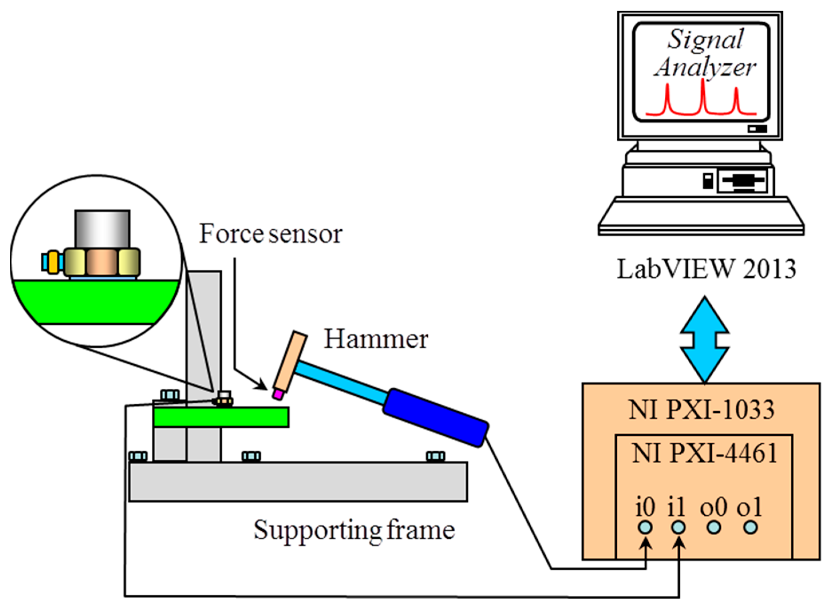
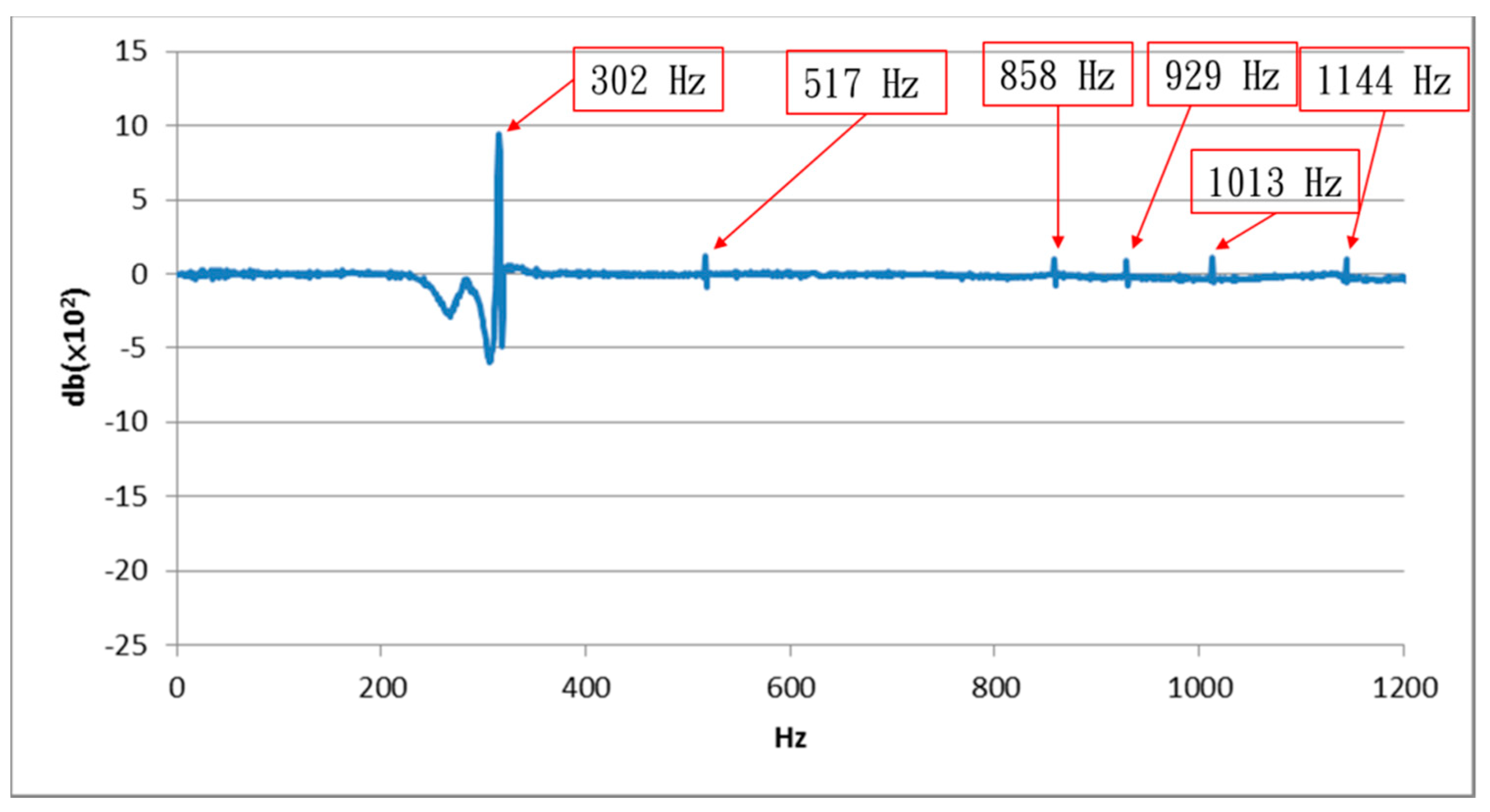
To verify the accuracy of the proposed method for the free vibration of thick composite cantilever plates, a rectangular composite plate comprising 332 layers of carbon/epoxy laminae was subjected to free vibration testing. A schematic description of the vibration test apparatus is shown in Figure 2. A detailed description of the fabrication, vibration testing, and material characterization of the plate is given in [73]. In the vibration test, one short side of the plate was clamped by a rigid fixture so that the plate could behave like a cantilever plate. The dimensions of the cantilever were a = 139.96 mm, b = 85.16 mm, and h = 27.16 mm with a/h = 5.15. During the vibration test, a hammer was used to strike the plate at different locations while a small accelerometer of 0.6 g was placed at a specific location. The vibration signals measured by the accelerometer were used to determine the frequency response spectra for the plate. The above testing procedure was repeated for several locations of the accelerometer. A typical frequency response spectrum is shown in Figure 3. The measured frequency response spectra were then used to extract the average values of the first six natural frequencies. The average values of the first six natural frequencies (fi, i = 1, …, 6) determined from all the measured frequency response spectra are given as follows: f1 = 302 Hz, f2 = 517 Hz, f3 = 858 Hz, f4 = 929 Hz, f5 = 1013 Hz, and f6 = 1144 Hz.
It is noted that the coefficients of variation of the first six natural frequencies are less than 7%.
Furthermore, the material properties of the composite lamina obtained from tests are given as E1 = 124.73 GPa, E2 = 5.43 GPa, ν12 = 0.30, G12 = 4.10 GPa, G23 = 0.67 GPa, G13 = 4.10 GPa, and ρ = 1570.47 kg/m3.
5. Results and Discussion
The proposed method is used to study the free vibration of several thin as well as thick composite cantilever plates the natural frequencies of which are available in the literature. First, a series of convergence tests were performed for thick plates with different length-to-thickness ratios to determine the appropriate number of terms, i.e., Ms and Ns, adopted in Equation (18). It is worth pointing out that Narita and Lessie used Equation (21) to study the free vibration of thin composite cantilever plates. They found that the use of Mb = Nb = 10 for approximating the thin plate deflection can make the solution converge. Hence, in this study, Mb = Nb = 10 is also used for approximating Wb. As for Ws, the square cantilever plate with zero fiber angles, a = 1 m, a/h = 5, and the following information about glass/epoxy are used to perform the convergence test:
E1 = 60.7 GPa, E2 = 24.8 GPa, ν12 = 0.23, G12 = 11.99 GPa, G23 = 11.99 GPa, G13 = 11.99 GPa, ρ = 1000 kg/m3, and E1/E2 = 2.45.
The convergence test results listed in Table 1 show that the natural frequencies of the plate converge when Mb = Nb = 10 and Ms = Ns = 5 which are also applicable to other plates with different fiber angles and length-to-thickness ratios.
The proposed method is then used to determine the natural frequencies of a thin square glass/epoxy cantilever plate with a fiber angle equal to 30° and aspect ratio a/h = 150. The predicted normalized natural frequencies are listed in Table 2 in comparison with those reported in the literature. The small differences between the normalized natural frequencies predicted using the present method and those obtained by Narita and Leissa imply that the shear deformation Ws has negligible effects on the natural frequencies of the plate. It is worth pointing out that for this case, the number of terms in Ws also has insignificant effects on the natural frequencies of the plate. For comparison purposes, the 2D Shell99 element of the commercial finite element code ANSYS [74] is also used to determine the natural frequencies of the plate. As shown in Table 2, the natural frequencies predicted using the present method are more accurate than those predicted using Shell99.
Next, the proposed method is used to determine the natural frequencies of symmetrically laminated graphite/epoxy cantilever plates with a/h = 73.2 and different fiber angles to compare with those obtained using other methods. The properties of the graphite/epoxy material are given as follows:
E1 = 112 GPa, E2 = 11 GPa, ν12 = 0.25, G12 = 4.48 GPa, G23 = 4.48 GPa, G13 = 4.48 GPa, ρ = 1500 kg/m3.
The natural frequencies of the composite cantilever plates with various lamination arrangements obtained using different methods are listed in Table 3, Table 4 and Table 5 for comparison.
The inspection of the differences between the experimental and theoretical normalized natural frequencies in Table 3, Table 4 and Table 5 shows that the present method can produce results closely matching the experimental data for all the composite plates under consideration. Furthermore, the fact that the present method can predict the first natural frequencies more accurately than the CPT reveals the significant effects of across-thickness shear deformation on the modal characteristics of the plates. It is noted that the value of E1/G13 = 25 gives the major contribution to the across-thickness shear deformation. Therefore, the through-thickness shear deformation effects on plate modal characteristics may become too significant to be neglected when the thickness of the cantilever plate or E1/G13 gets larger.
The proposed method is then used to predict the natural frequencies of thick cantilever plates. First, consider the free vibration of a thick isotropic cantilever plate with a/h = 5. The first four normalized natural frequencies of the plate are listed in Table 6 in comparison with the experimental data available in the literature. It is noted that the results obtained using the present method are acceptable. In particular, for the first mode, the percentage difference between the first theoretical and experimental normalized natural frequencies is less than 1.8% while that of the finite element method (FETM) is larger than 11.24%.
Next, the proposed method is used to determine the natural frequencies of the [0°]332 carbon/epoxy cantilever plate which has been tested. The theoretical natural frequencies predicted using the present method are compared with the experimental ones as tabulated in Table 7. It is noted that for comparison purposes, the 2D Shell99 and 3D Solid186 elements of ANSYS have also been used to determine the natural frequencies. The comparison shows that both the present method and ANSYS, no matter whether 2D or 3D elements, are able to produce acceptable results. Compared with the experimental natural frequencies, the absolute percentage differences for 3D Solid186, the present method, and 2D Shell99 are less than or equal to 5.79, 6.36, and 8.68%, respectively.
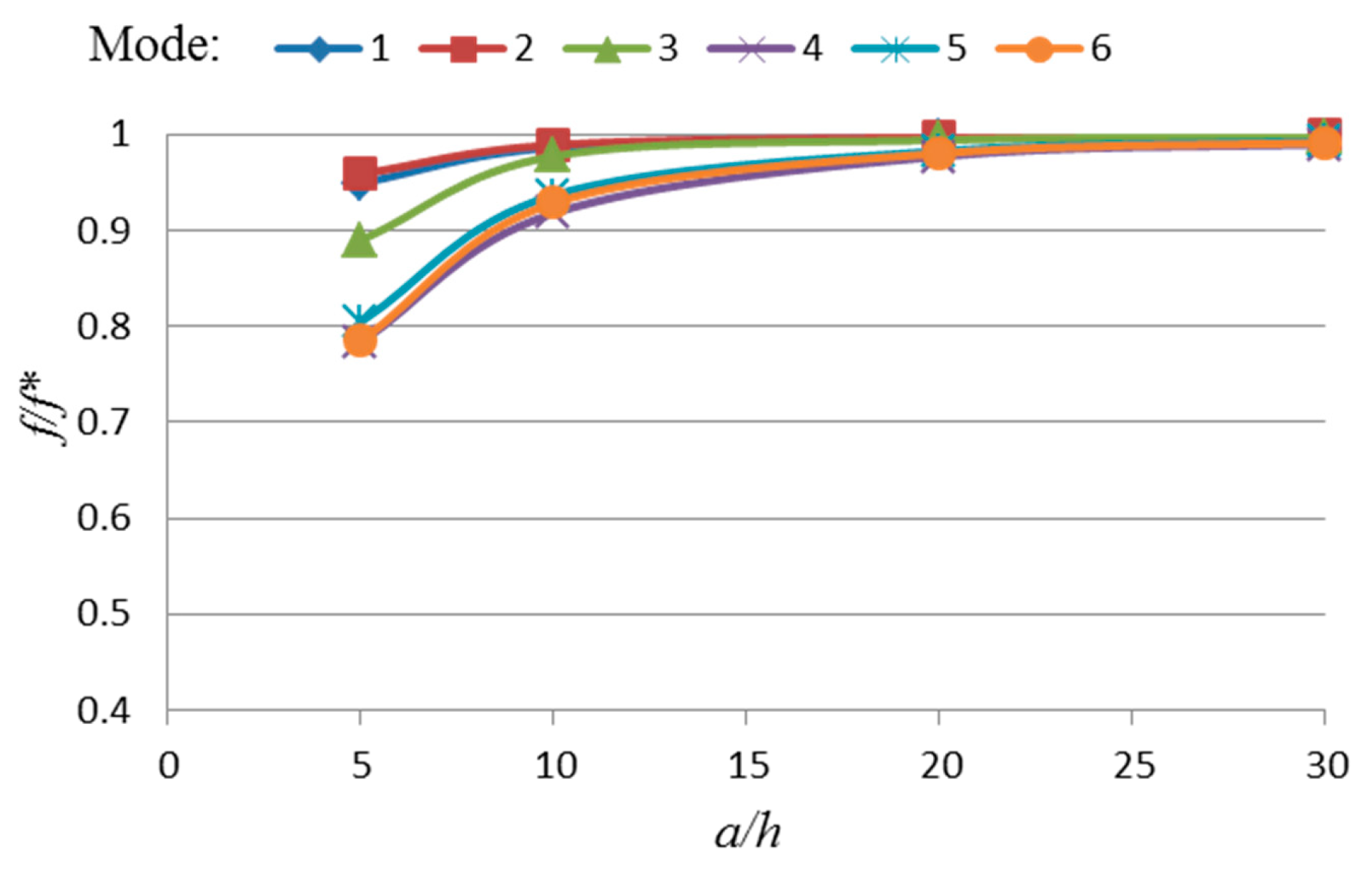
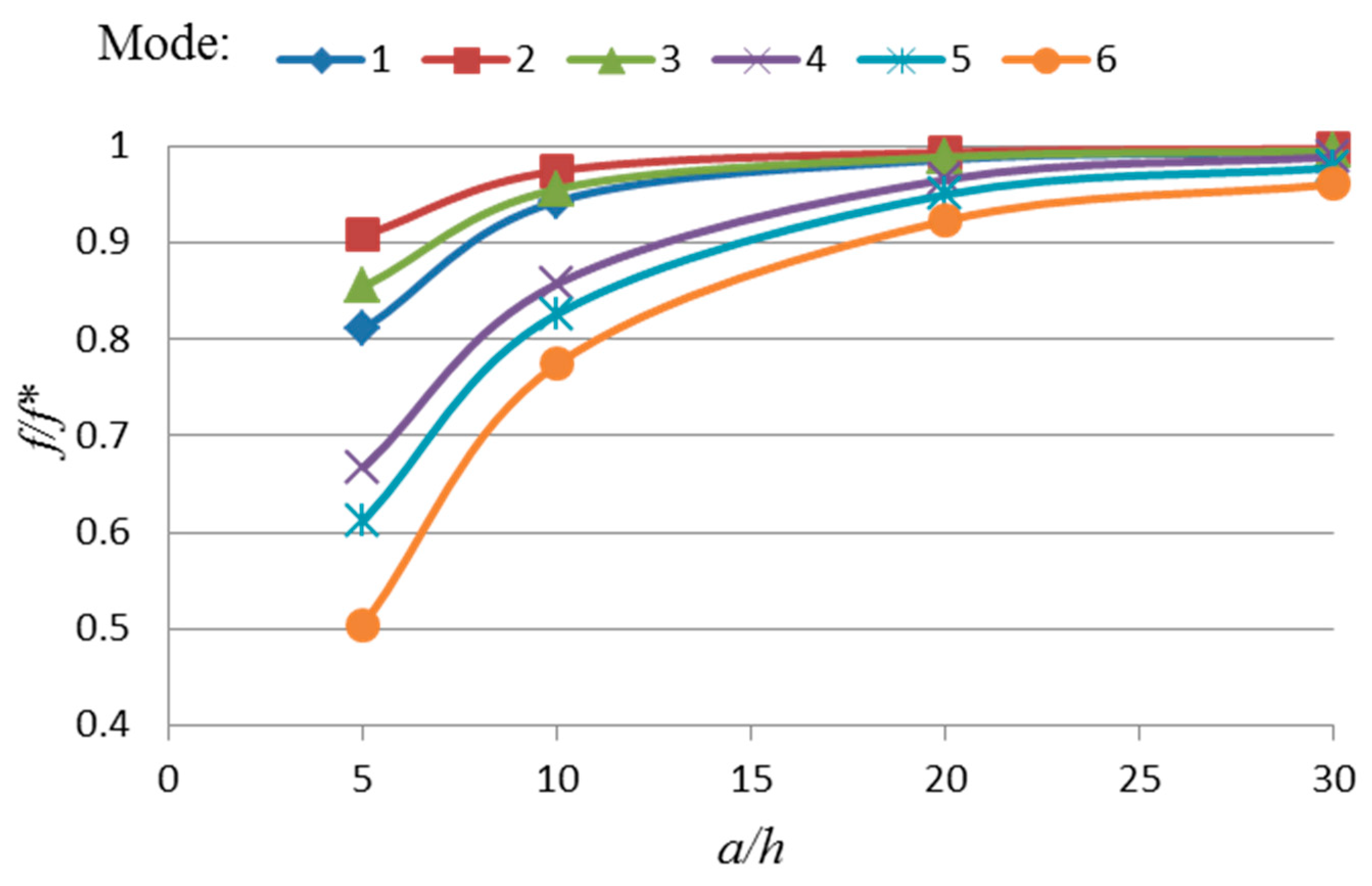
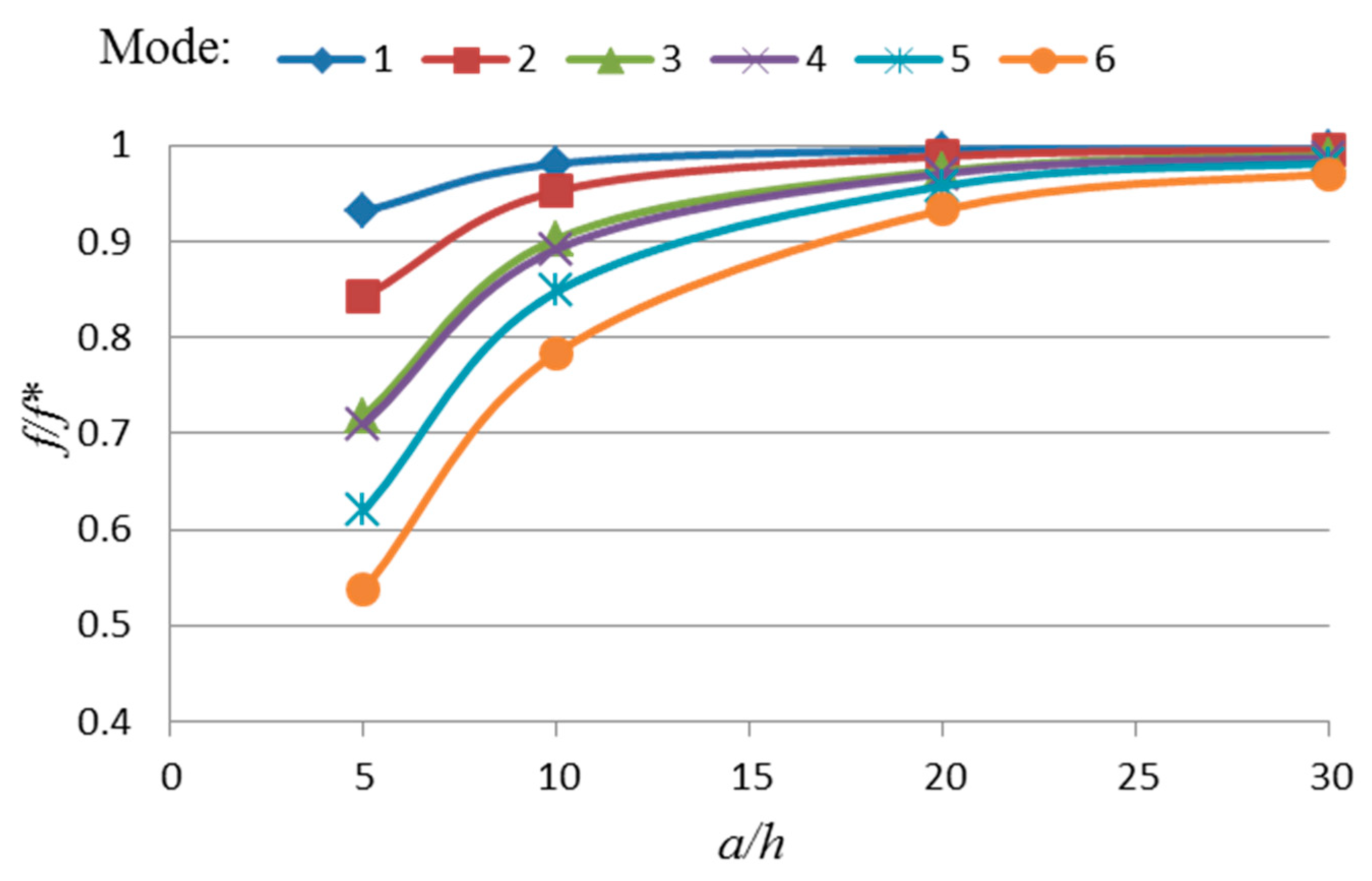
The present method is used to study the effects of length-to-thickness ratio (a/h) on the natural frequencies of carbon/epoxy plates with different fiber angles. Consider the first six natural frequencies of the composite cantilever plates with different length-to-thickness ratios and lamination arrangements. Herein, the natural frequency f determined using the present method is normalized with respect to the f* determined using the CPT. The relations between the normalized natural frequency and length-to-thickness ratio for the [0]8, [0, 902, 0]s, and [45, −452, 45]s plates are shown in Figure 4, Figure 5 and Figure 6, respectively. It is noted that the plate thickness has significant effects on the natural frequencies for all the plates. In particular, each normalized natural frequency becomes lower as the length-to-thickness gets smaller and such effects become more prominent for higher modes.
With respect to engineering applications, the natural frequencies predicted using the present method together with the natural frequencies determined experimentally can be used to identify material constants for the quality control of composite plates after fabrication or health assessment of existing cantilever composite plates. Regarding an existing cantilever plate having been operated in a severe environment for some time, the degradation of the constituent material will cause the values of the plate’s natural frequencies to decrease. In practice, the current natural frequencies of the plate can be determined via vibration testing. The deviations of the current natural frequencies from the original ones can then be used to identify the current material constants such as E1, E2, and G12 for the health assessment of the plate. It is a common practice to use several measured natural frequencies in an optimization method to identify all the material constants simultaneously. However, for some material constant identification problems, the search for the true solution in the identification process may encounter difficulties in making the solution converge, or the adopted search algorithm, in terms of computation time, is too expensive to be used for practical applications. Herein, for illustration, a procedure is presented to identify the current material constants of laminated composite cantilever plates with different length-to-thickness ratios. First, consider the sensitivity analysis of natural frequencies subject to the variation of each material constant for a graphite/epoxy [0]8 cantilever plate with a/h = 120. The percentage changes in the natural frequencies for a 20% reduction in each material constant are listed in Table 8.
It is noted that each material constant may have effects of different extents on the natural frequencies. For instance, compared with other material constants, Young’s modulus E1 has the most prominent effects on the first natural frequency of the plate while Poisson’s ratio v12 has insignificant effects on the first five natural frequencies. The information will be used in the identification procedure to estimate the current material constants E1, E2, and G12. For illustrating the idea of the proposed identification procedure, rather than testing, the current “measured” natural frequencies are determined using the present method. The first five original and “measured” natural frequencies associated with, respectively, the original and degraded material constants are assumed to be as follows:
- Natural frequency (Hz)
- Original: f1 = 11.66, f2 = 15.01, f3 = 31.86, f4 = 69.96, f5 = 72.90;
- Measured: f1* = 10.43, f2* = 13.42, f3* = 28.49, f4* = 62.58, f5* = 65.20.
- and material constants
- Original: E1 = 112.00 GPa, E2 = 11.00 GPa, ν12 = 0.2, G12 = 4.48 GPa;
- Degraded: E1 = 89.60 GPa, E2 = 8.80 GPa, ν12 = 0.2, G12 = 3.58 GPa.
For the material degradation assessment of thin plates, it is reasonable to assume v12 to be constant and G12 = G13 = G23. After reviewing the sensitivity analysis results listed in Table 9, it is possible that a chosen natural frequency can be used to estimate a particular material constant. In this case, the natural frequency f1, f2, or f4 will be used individually to estimate, respectively, material constant E1, G12, or E2 using a minimization technique. First, let the original material constants be X(1) = E1, X(2) = E2, and X(3) = G12. The updated material constant X(i)* is equal to q(i) X(i) in which the parameter q(i) satisfies the condition of (ql < q < qu) with ql = 0 and qu = 1. The updated material constants are used in the proposed method to predict the selected natural frequency f(q(i)) which depends on the chosen values of the parameters q(i). The minimization procedure for identifying the current E1 using the first natural frequency is given as follows:
- Step 1. Calculate the upper bound frequency fu using q(1) = q(2) = q(3) = 1 and lower bound frequency fl using q(1) = 0.1 and q(2) = q(3) = 1. Set qu = 1 and ql = 0.1.
- Step 2. Set q(1) = 0.5, q(2) = q(3) = 1.
- Step 3. Let X(i)* = q(i)X(i); choose f* = f1*.
- Step 4. Calculate the error function e(q(i)) = {f(q(i)) − f*}/f*. If e < 0.01, go to Step 8.
- Step 5. If e (q(i)) > 0, then let qu = q(1) and calculate the upper bound frequency fu for qu. Otherwise, if e (q(i)) < 0, then let ql = q(1) and calculate the lower bound frequency fl for ql.
- Step 6. Update q(1) = ql + (f* − fl) (qu − ql)/(fu − fl).
- Step 7. Go to Step 4.
- Step 8. Stop the iteration.
After performing the above minimization procedure, the best estimate of the current E1 has been attained with q(1) = 0.7993. Once the best estimate of E1 has been attained, the above minimization procedure can be used to find the best estimate of the current G12 by initiating q(1) = 0.7993, q(2) = 1, q(3) = 0.5, and f* = f2* in the minimization process. Similarly, once the best estimates of the current E1 and G12 are available, i.e., q(1) = 0.7993 and q(3) = 0.7957, the above minimization procedure can be used to find the best estimate of the current E2 by initiating q(1) = 0.7993, q(2) = 0.5, q(3) = 0.7957, and f* = f4* in the minimization process. It is noted that the proposed minimization procedure requires fewer than 10 iterations to identify each current material constant. The identified current material constants are listed in Table 9 in comparison with the actual ones. It is noted that the proposed material constant identification method can produce good results for a thin plate with a maximum error of less than 0.6%.
The proposed minimization procedure is then used to identify the material constants of the same [0°]8 cantilever plate but with a/h = 20. Again, consider the sensitivity analysis of natural frequencies subject to the variation of each material constant for the plate. The percentage changes in the natural frequencies for a 20% reduction in each material constant are listed in Table 10.
It is noted that each material constant may have effects of different extents on the natural frequencies. For instance, with respect to the first natural frequency, Young’s modulus E1 has the most prominent effects on the first natural frequency of the plate while the effects of the other material constants are insignificant. The sensitivity information will be used in the identification procedure to estimate the current material constants E1, E2, G12, and G23. For illustration purposes, the current “measured” natural frequencies are again determined using the present method instead of testing. The first five original and “measured” natural frequencies associated with, respectively, the original and degraded material constants are assumed to be as given below. The original and degraded material constants used in this case are the same as those of a/h = 120.
- Natural frequency (Hz):
- Original: f1 = 69.10, f2 = 89.53, f3 = 189.14, f4 = 404.19, f5 = 410.12;
- Measured: f1* = 61.77, f2* = 80.05, f3* = 169.14, f4* = 361.37, f5* = 366.89.
Herein, following the same idea of the proposed current material constant identification procedure, the first “measured” natural frequency is used to identify the current E1, the second to identify G12, the third to identify E2, and the fourth to identify G23. The best estimates of the current material constants are listed in Table 11 in comparison with the actual ones. It is noted that the present material constant identification procedure can produce acceptable results for the relatively thick plate, with a maximum error of less than 4.5%.
The above examples have shown that the information of frequency sensitivity analysis can greatly reduce the number of material constants required to be used in the minimization process so that only a few iterations, usually fewer than 10, are needed to identify any material constant. The attainment of good estimates of material constants in an efficient and effective way is the merit of the proposed material constant identification procedure. It is also worth pointing out that the proposed procedure can be applied to identify the material constants of laminated composite plates with other boundary conditions.
6. Conclusions
A new SFSDT-based Ritz method has been presented to analyze the free vibration of rectangular thick laminated composite cantilever plates. In the proposed method, the two sets of characteristic functions used to model, respectively, the two deflection components, namely, bending and through-thickness shear-deformation-induced deflections, for forming the total plate deflection, are required to be independent and satisfy the displacement and force conditions at the fixed edge of the plate. It has been shown that the selection of the polynomial type characteristic functions for modeling the bending-induced deflection, and the trigonometric type characteristic functions for the through-thickness shear-deformation-induced deflection is applicable for the free vibration of thin as well as thick composite plates. The existing theoretical and experimental results of several composite plates under free vibration have been used to verify the accuracy of the proposed method. In particular, the proposed method can predict exactly the same natural frequencies as those reported in the literature for thin symmetrically laminated composite plates. As for thick composite plates, the present method can predict the first six natural frequencies with percentage differences of less than 6.4% when compared with the experimental natural frequencies of a thick composite plate with a 0° fiber angle and length-to-thickness ratio equal to 5.15. A number of square composite cantilever plates with different length-to-thickness ratios and fiber angles have been analyzed using the proposed method to study the effects of through-thickness shear deformation on the natural frequencies of the plates. It has been shown that irrespective of fiber angles, the decrease in length-to-thickness ratio can cause significant decreases in the natural frequencies of the plates, especially for higher modes. In particular, for the sixth natural frequency of the graphite/epoxy [0, 902, 0]s square plate with a length-to-thickness ratio equal to 5, the decrease in the natural frequency is about 50%. For application illustration, the proposed method has been used in the assessment of material degradation of composite cantilever plates. A novel procedure has been presented to identify the material constants of degraded composite cantilever plates using the information obtained from the sensitivity analysis of natural frequencies subjected to any material constant variation. In the proposed procedure, the number of design variables to be determined in a minimization technique has been greatly reduced so that the convergence problems which may have been encountered in many existing material constant identification methods can be circumvented. The examples have illustrated that the proposed material constant identification procedure can produce good estimates of the true current E1, E2, and G12 with errors less than 4.5%, and in identifying each material constant, fewer than 10 iterations are needed to produce a good estimate of the true value.
Author Contributions
Conceptualization, T.Y.K.; methodology, T.Y.K.; software, C.W.L.; validation, C.W.L. and T.Y.K.; formal analysis, C.W.L.; investigation, C.W.L. and T.Y.K.; resources, T.Y.K.; data curation, C.W.L.; writing—original draft preparation, T.Y.K.; writing—review and editing, T.Y.K.; supervision, T.Y.K.; project administration, T.Y.K.; funding acquisition, T.Y.K. All authors have read and agreed to the published version of the manuscript.
Funding
This research was funded by National Science and Technology Council of the Republic of China under the grant MOST 111-2221-E-A49-109.
Institutional Review Board Statement
The study was conducted in accordance with the Declaration of Helsinki, and approved by the Institutional Review Board of National Yang Ming Chiao Tung University (protocol code: Hsin Chu 300 and date of approval: 16 April 2023).
Informed Consent Statement
No new data were created.
Data Availability Statement
No new data were created.
Conflicts of Interest
The authors declare no conflict of interest.
Appendix A
Elements of system matrices:
- 1.
- Mass matrix M
- q = 1, 2, 3, …, Rm
- r = 1, 2, 3, …, Rm
- q = Rm + qi + 2(qi − 1)Ns; qi = 1, 2, 3, …, Ms
- r = 1, 2, 3, …, Rm
- q = Rm + (qi − 1) + 2(qi − 1)Ns + 2qj; qi = 1, 2, 3, …, Ms; qj = 1, 2, 3, …, Ns
- r = 1, 2, 3, …, Rm
- q = Rm + qi + 2(qi − 1)Ns + 2qj; qi = 1, 2, 3, …, Ms; qj = 1, 2, 3, …, Ns
- r = 1, 2, 3, …, Rm
- q = 1, 2, 3, …, Rm
- r = Rm + qi + 2(qi − 1)Ns; qi = 1, 2, 3, …, Ms
- q = Rm + qi + 2(qi − 1)Ns; qi = 1, 2, 3, …, Ms
- r = Rm + qi + 2(qi − 1)Ns; qi = 1, 2, 3, …, Ms
- q = Rm + (qi − 1) + 2(qi − 1)Ns + 2qj; qi = 1, 2, 3, …, Ms; qj = 1, 2, 3, …, Ns
- r = Rm + qi + 2(qi − 1)Ns; qi = 1, 2, 3, …, Ms
- q = Rm + qi + 2(qi − 1)Ns + 2qj; qi = 1, 2, 3, …, Ms; qj = 1, 2, 3, …, Ns
- r = Rm + qi + 2(qi − 1)Ns; qi = 1, 2, 3, …, Ms
- q = 1, 2, 3, …, Rm
- r = Rm + (qi − 1) + 2(qi − 1)Ns + 2qj; qi = 1, 2, 3, …, Ms; qj = 1, 2, 3, …, Ns
- q = Rm + qi + 2(qi − 1)Ns; qi = 1, 2, 3, …, Ms
- r = Rm + (qi − 1) + 2(qi − 1)Ns + 2qj; qi = 1, 2, 3, …, Ms; qj = 1, 2, 3, …, Ns
- q = Rm + (qi − 1) + 2(qi − 1)Ns + 2qj; qi = 1, 2, 3, …, Ms; qj = 1, 2, 3, …, Ns
- r = Rm + (qi − 1) + 2(qi − 1)Ns + 2qj; qi = 1, 2, 3, …, Ms; qj = 1, 2, 3, …, Ns
- q = Rm + qi + 2(qi − 1)Ns + 2qj; qi = 1, 2, 3, …, Ms; qj = 1, 2, 3, …, Ns
- r = Rm + qi + 2(qi − 1)Ns; qi = 1, 2, 3, …, Ms
- q = 1, 2, 3, …, Rm
- r = Rm + qi + 2(qi − 1)Ns + 2qj; qi = 1, 2, 3, …, Ms; qj = 1, 2, 3, …, Ns
- q = Rm + qi + 2(qi − 1)Ns; qi = 1, 2, 3, …, Ms
- r = Rm + qi + 2(qi − 1)Ns + 2qj; qi = 1, 2, 3, …, Ms; qj = 1, 2, 3, …, Ns
- q = Rm + (qi − 1) + 2(qi − 1)Ns + 2qj; qi = 1, 2, 3, …, Ms; qj = 1, 2, 3, …, Ns
- r = Rm + qi + 2(qi − 1)Ns + 2qj; qi = 1, 2, 3, …, Ms; qj = 1, 2, 3, …, Ns
- q = Rm + qi + 2(qi − 1)Ns + 2qj; qi = 1, 2, 3, …, Ms; qj = 1, 2, 3, …, Ns
- r = Rm + qi + 2(qi − 1)Ns + 2qj; qi = 1, 2, 3, …, Ms; qj = 1, 2, 3, …, Ns
- 2.
- Stiffness matrix K
- q = 1, 2, 3, …, Rm
- r = 1, 2, 3, …, Rm
- q = Rm + qi + 2(qi − 1)Ns; qi = 1, 2, 3, …, Ms
- r = Rm + qi + 2(qi − 1)Ns; qi = 1, 2, 3, …, Ms
- q = Rm + (qi − 1) + 2(qi − 1)Ns + 2qj; qi = 1, 2, 3, …, Ms; qj = 1, 2, 3, …, Ns
- r = Rm + qi + 2(qi − 1)Ns; qi = 1, 2, 3, …, Ms
- q = Rm + qi + 2(qi − 1)Ns + 2qj; qi = 1, 2, 3, …, Ms; qj = 1, 2, 3, …, Ns
- r = Rm + qi + 2(qi − 1)Ns; qi = 1, 2, 3, …, Ms
- q = Rm + qi + 2(qi − 1)Ns; qi = 1, 2, 3, …, Ms
- r = Rm + (qi − 1) + 2(qi − 1)Ns + 2qj; qi = 1, 2, 3, …, Ms; qj = 1, 2, 3, …, Ns
- q = Rm + (qi − 1) + 2(qi − 1)Ns + 2qj; qi = 1, 2, 3, …, Ms; qj = 1, 2, 3, …, Ns
- r = Rm + (qi − 1) + 2(qi − 1)Ns + 2qj; qi = 1, 2, 3, …, Ms; qj = 1, 2, 3, …, Ns
- q = Rm + qi + 2(qi − 1)Ns + 2qj; qi = 1, 2, 3, …, Ms; qj = 1, 2, 3, …, Ns
- r = Rm + (qi − 1) + 2(qi − 1)Ns + 2qj; qi = 1, 2, 3, …, Ms; qj = 1, 2, 3, …, Ns
- q = Rm + qi + 2(qi − 1)Ns; qi = 1, 2, 3, …, Ms
- r = Rm + qi + 2(qi − 1)Ns + 2qj; qi = 1, 2, 3, …, Ms; qj = 1, 2, 3, …, Ns
- q = Rm + (qi − 1) + 2(qi − 1)Ns + 2qj; qi = 1, 2, 3, …, Ms; qj = 1, 2, 3, …, Ns
- r = Rm + qi + 2(qi − 1)Ns + 2qj; qi = 1, 2, 3, …, Ms; qj = 1, 2, 3, …, Ns
- q = Rm + qi + 2(qi − 1)Ns + 2qj; qi = 1, 2, 3, …, Ms; qj = 1, 2, 3, …, Ns
- r = Rm + qi + 2(qi − 1)Ns + 2qj; qi = 1, 2, 3, …, Ms; qj = 1, 2, 3, …, Ns
- 3.
- wherewith
References
- Kam, T.Y.; Lai, F.M. Design of laminated composite plates for optimal dynamic characteristics using a constrained global optimization technique. Comput. Methods Appl. Mech. Eng. 1995, 121, 389–402. [Google Scholar] [CrossRef]
- Cho, H.K. Design optimization of laminated composite plates with static and dynamic considerations in hygrothermal environments. Int. J. Precis. Eng. Manuf. 2013, 14, 1387–1394. [Google Scholar] [CrossRef]
- Kam, T.Y.; Chang, R.R. Optimal design of laminated composite plates with dynamic and static considerations. Comput. Struct. 1989, 32, 387–393. [Google Scholar] [CrossRef]
- Liu, Q.; Paavola, J. Lightweight design of composite laminated structures with frequency constraint. Compos. Struct. 2016, 156, 356–360. [Google Scholar] [CrossRef]
- Muc, A. Natural Frequencies of Rectangular Laminated Plates—Introduction to Optimal Design in Aeroelastic Problems. Aerospace 2018, 5, 95. [Google Scholar] [CrossRef]
- Kam, T.Y.; Lee, T.Y. Detection of Cracks from Modal Test Data. Eng. Fract. Mech. 1992, 42, 381–387. [Google Scholar] [CrossRef]
- Kam, T.Y.; Lee, T.Y. Crack Size Identification Using an Expanded Mode Method. Int. J. Solids Struct. 1994, 31, 925–940. [Google Scholar] [CrossRef]
- Xu, G.Y.; Zhu, W.D.; Emory, B.H. Experimental and Numerical Investigation of Structural Damage Detection Using Changes in Natural Frequencies. J. Vib. Acoust. 2007, 129, 686–700. [Google Scholar] [CrossRef]
- Kim, J.T.; Ryu, Y.S.; Cho, H.M.; Stubbs, N. Damage identification in beam-type structures: Frequency-based method vs mode-shape-based method. Eng. Struct. 2003, 25, 57–67. [Google Scholar] [CrossRef]
- Vestroni, F.; Capecchi, D. Damage detection in beam structures based on frequency measurements. J. Eng. Mech. 2000, 126, 761–768. [Google Scholar] [CrossRef]
- Lee, J. Identification of multiple cracks in a beam using natural frequencies. J. Sound Vib. 2009, 320, 482–490. [Google Scholar] [CrossRef]
- White, C.; Li, H.C.; Whittingham, B.; Herszberg, I.; Mouritz, A.P. Damage detection in repairs using frequency response techniques. Compos. Struct. 2009, 87, 175–181. [Google Scholar] [CrossRef]
- Hwang, S.F.; Wu, J.C.; He, R.S. Identification of effective elastic constants of composite plates based on a hybrid genetic algorithm. Compos. Struct. 2009, 90, 217–224. [Google Scholar] [CrossRef]
- Yan, A.M.; Golinval, J.C. Model updating based on frequency response functions using a general finite element code. Eur. J. Mech. Environ. Eng. 2003, 48, 149–162. [Google Scholar]
- Araujo, A.L.; Soares, C.M.M.; DeFreitas, M.J.M. Characterization of material parameters of composite plate specimens using optimization and experimental vibrational data. Compos. Part B Eng. 1996, 27, 185–191. [Google Scholar] [CrossRef]
- Lee, C.R.; Kam, T.Y. System identification of partially restrained composite plates using measured natural frequencies. J. Eng. Mech. 2006, 132, 841–850. [Google Scholar] [CrossRef]
- Lee, C.R.; Kam, T.Y. Identification of mechanical properties of elastically restrained laminated composite plates using vibration data. J. Sound Vib. 2006, 295, 999–1016. [Google Scholar] [CrossRef]
- Lee, C.R.; Kam, T.Y.; Sun, S.J. Free-vibration analysis and material constants identification of laminated composite sandwich plates. J. Eng. Mech. 2007, 133, 874–886. [Google Scholar] [CrossRef]
- Schwaar, M.; Gmur, T.; Frieden, J. Modal numerical-experimental identification method for characterising the elastic and damping properties in sandwich structures with a relatively stiff core. Compos. Struct. 2012, 94, 2227–2236. [Google Scholar] [CrossRef]
- Lauwagie, T.; Sol, H.; Heylen, W.; Roebben, G. Determination of the inplane elastic properties of the different layers of laminated plates by means of vibration testing and model updating. J. Sound Vib. 2004, 274, 529–546. [Google Scholar] [CrossRef]
- Nayan, A.; Kam, T.Y. Sound Enhancement of Orthotropic Sound Radiation Plates Using Line Loads and Considering Resonance Characteristics. Acoustics 2021, 3, 642–664. [Google Scholar] [CrossRef]
- Jiang, C.H.; Kam, T.Y.; Chang, Y.H. Sound radiation of panel-form loudspeaker using flat voice coil for excitation. Appl. Acoust. 2017, 116, 375–389. [Google Scholar] [CrossRef]
- Jiang, C.H.; Chang, Y.H.; Kam, T.Y. Optimal design of rectangular composite flat-panel sound radiators considering excitation location. Compos. Struct. 2014, 108, 65–76. [Google Scholar] [CrossRef]
- Crawley, E.F.; Dugundji, J. Frequency determination and non-dimensionalization for composite cantilever plates. J. Sound Vib. 1980, 72, 1–10. [Google Scholar] [CrossRef]
- Liu, W.H.; Huang, C.C. Free vibrations of thick cantilever laminated plates with step-change of thickness. J. Sound Vib. 1994, 169, 601–618. [Google Scholar] [CrossRef]
- Jaehwan, K.; Vasundara, V.V.; Vijay, K.V.; Xiao-Qi, B. Finite-element modeling of a smart cantilever plate and comparison with experiments. Smart Mater. Struct. 1996, 5, 165–170. [Google Scholar]
- Seok, J.; Tiersten, H.F.; Scarton, H.A. Free vibrations of rectangular cantilever plates. Part1: Out-of plane motion. J. Sound Vib. 2004, 271, 131–146. [Google Scholar] [CrossRef]
- Dokainish, M.A.; Rawtani, S. Vibration analysis of rotating cantilever plates. Int. J. Numer. Methods Eng. 1971, 3, 233–248. [Google Scholar] [CrossRef]
- Karmakar, A.; Sinha, P.K. Finite element free vibration analysis of rotating laminated composite pretwisted cantilever plates. J. Reinf. Plast. Compos. 1997, 16, 1461–1490. [Google Scholar] [CrossRef]
- Kılıc, O.; Aktas, A.; Husnu, M.D. An investigation of the effects of shear on the deflection of an orthotropic cantilever beam by the use of anisotropic elasticity theory. Compos. Sci. Technol. 2001, 61, 2055–2061. [Google Scholar] [CrossRef]
- Yoo, H.H.; Kim, S.K. Free vibration analysis of rotating cantilever plates. AIAA J. 2002, 40, 2188–2196. [Google Scholar] [CrossRef]
- Yoo, H.H.; Pierre, C. Modal characteristic of a rotating rectangular cantilever plate. J. Sound Vib. 2003, 259, 81–96. [Google Scholar] [CrossRef]
- Wang, G.; Wereley, N.M. Free Vibration Analysis of Rotating Blades with Uniform Tapers. AIAA J. 2004, 42, 1531–1541. [Google Scholar] [CrossRef]
- Hamza-Cherif, S.M. Free vibration analysis of rotating cantilever plates using the p-version of the finite element method. Struct. Eng. Mech. 2006, 22, 151–167. [Google Scholar] [CrossRef]
- Hashemi, S.H.; Farhadi, S.; Carra, S. Free vibration analysis of rotating thick plates. J. Sound Vib. 2009, 323, 366–384. [Google Scholar] [CrossRef]
- Moon, K.K.; Dong-Ho, Y. Free vibration analysis of cantilever plate partially submergedinto a fluid. J. Fluids Struct. 2013, 40, 25–41. [Google Scholar]
- Dozio, L.; Carrera, E. A variable kinematic Ritz formulation for vibration study of quadrilateral plates with arbitrary thickness. J. Sound Vib. 2011, 330, 4611–4632. [Google Scholar] [CrossRef]
- Vescovini, R.; Dozio, L.; D’Ottavio, M.; Polit, O. On the application of the Ritz method to free vibration and buckling analysis of highly anisotropic plates. Compos. Struct. 2018, 192, 460–474. [Google Scholar] [CrossRef]
- Narita, Y.; Leissa, A.W. Frequencies and mode shapes of cantilevered laminated composite plates. J. Sound Vib. 1992, 154, 161–172. [Google Scholar] [CrossRef]
- Cupial, P. Calculation of the natural frequencies of composite plates by the Rayleigh-Ritz method with orthogonal polynomials. J. Sound Vib. 1992, 201, 385–387. [Google Scholar] [CrossRef]
- Al-Obeid, A.; Cooper, J.E. A Rayleigh-Ritz approach for estimation of the dynamic properties of symmetric composite plates with general boundary conditions. Compos. Sci. Technol. 1995, 53, 289–299. [Google Scholar] [CrossRef]
- Aydogdu, M.; Filiz, S. Vibration analysis of symmetric laminated composite plates with attached mass. Mech. Adv. Mater. Struct. 2016, 23, 136–145. [Google Scholar] [CrossRef]
- Shojaee, S.N.; Valizadeh; Izadpanah, E.; Bui, T.; Van, V.T. Free vibration and buckling analysis of laminated composite plates using the NURBS-based isogeometric finite element method. Compos. Struct. 2012, 94, 1677–1693. [Google Scholar] [CrossRef]
- Basavaraj, S.B.; Kamal, M.B.; Sudhakar, A.K. Natural frequencies of a multilayer SMA laminated composite cantilever plate. Smart Mater. Struct. 2006, 15, 1021–1032. [Google Scholar]
- Quintana, M.V.; Raffo, J.L. A variational approach to vibrations of laminated composite plates with a line hinge. Eur. J. Mech. A/Solids 2019, 73, 11–21. [Google Scholar] [CrossRef]
- Kam, T.Y.; Jiang, C.H.; Lee, P.Y. Vibro-acoustic Formulation of Elastically Restrained Shear Deformable Stiffened Plate. J. Compos. Struct. 2012, 94, 3132–3141. [Google Scholar] [CrossRef]
- Malekzadeh, K.; Sayyidmousavi, A. Free Vibration Analysis of Sandwich Plates with a Uniformly Distributed Attached Mass, Flexible Core, and Different Boundary. J. Sandw. Struct. Mater. 2010, 12, 709–732. [Google Scholar] [CrossRef]
- Carrera, E.; Fazzolari, F.A.; Demasi, L. Vibration analysis of anisotropic simply supported plates by using variable kinematic and Rayleigh-Ritz method. J. Vib. Acoust. 2011, 133, 061017-1–061017-16. [Google Scholar] [CrossRef]
- Kiani, Y.; Żur, K.K. Free vibrations of graphene platelet reinforced composite skew plates resting on point supports. Thin-Walled Struct. 2022, 176, 109363. [Google Scholar] [CrossRef]
- Khandan, R.; Noroozi, S.; Sewell, P.; Vinney, J. The development of laminated composite plate theories: A review. J. Mater. Sci. 2012, 47, 5901–5910. [Google Scholar] [CrossRef]
- Ghugal, Y.M.; Shimpi, R.P. A review of refined shear deformation theories for isotropic and anisotropic laminated beams. J. Reinf. Plast. Compos. 2001, 20, 255–272. [Google Scholar] [CrossRef]
- Mindlin, R.D. Influence of Rotatory Inertia and Shear on Flexural Motions of Isotropic, Elastic Plates. J. Appl. Mech. 1951, 18, 31–38. [Google Scholar] [CrossRef]
- Reissner, E. The effect of transverse shear deformation on the bending of elastic plates. J. Appl. Mech. 1945, 12, 69–77. [Google Scholar] [CrossRef]
- Prabhu, M.R.; Davalos, J.F. Static shear correction factor for laminated rectangular beams. Compos. Part B 1996, 27B, 285–293. [Google Scholar]
- Hadavinia, H.; Gordnian, K.; Karwatzki, J.; Aboutorabi, A. Deriving Shear Correction Factor for Thick Laminated Plates Using the Energy Equivalence Method. SDHM Struct. Durab. Health Monit. 2006, 2, 197–206. [Google Scholar]
- Whitney, J.M. Shear correction factors for orthotropic laminates under static load. J. Appl. Mech. 1973, 40, 302–304. [Google Scholar] [CrossRef]
- Pai, P.G.F. A new look at shear correction factors and warping functions of anisotropic laminates. J. Solids Struct. 1995, 32, 2295–2313. [Google Scholar] [CrossRef]
- Chatterjee, S.N.; Kulkarni, S.V. Shear correction factors for laminated plates. AIAA J. 1979, 17, 498–499. [Google Scholar] [CrossRef]
- Thai, H.T.; Choi, D.H. A simple first-order shear deformation theory for the bending and free vibration analysis of functionally graded plates. Compos. Struct. 2013, 101, 332–340. [Google Scholar] [CrossRef]
- Thai, H.T.; Choi, D.H. A simple first-order shear deformation theory for laminated composite plates. Compos. Struct. 2013, 106, 754–763. [Google Scholar] [CrossRef]
- Thai, H.T.; Nguyen, T.K.; Vo, T.P.; Lee, J. Analysis of functionally graded sandwich plates using a new first-order shear deformation theory. Eur. J. Mech. A/Solids 2014, 45, 211–225. [Google Scholar] [CrossRef]
- Senjanović, I.; Nikola, V.; Cho, D.S. A new finite element formulation for vibration analysis of thick plates. Int. J. Nav. Archit. Ocean Eng. 2015, 7, 324–345. [Google Scholar] [CrossRef]
- Shimpi, R.P.; Patel, H.G.; Arya, H. New first-order shear deformation plate theories. J. Appl. Mech. ASME 2007, 74, 523–533. [Google Scholar] [CrossRef]
- Ho, C.N.; Tsai, Y.M.; Kam, T.Y. Finite element vibration analysis of composite plates based on the simple first order shear deformation theory. Proc. Asian Jt. Symp. Aerosp. Eng. 2018, 2018, 166–170. [Google Scholar]
- Park, M.W.; Choi, D.H. A two-variable first-order shear deformation theory considering in-plane rotation for bending, buckling and free vibration analyses of isotropic plates. Appl. Math. Model. 2018, 61, 49–71. [Google Scholar] [CrossRef]
- Thai, H.T.; Park, M.; Choi, D.H. A simple refined theory for bending, buckling, and vibration of thick plates resting on elastic foundation. Int. J. Mech. Sci. 2013, 73, 40–52. [Google Scholar] [CrossRef]
- Duc, D.H.; Thom, D.V.; Cong, P.H.; Minh, P.V.; Nguyen, N.X. Vibration and static buckling behavior of variable thickness flexoelectric nanoplates. Mech. Based Des. Struct. Mach. 2022, 2022, 2088558. [Google Scholar] [CrossRef]
- Adim, B.; Daouadji, T.H.; Rabahi, A. A simple higher order shear deformation theory for mechanical behavior of laminated composite plates. Int. J. Adv. Struct. Eng. 2016, 8, 103–117. [Google Scholar] [CrossRef]
- Do, V.T.; Pham, V.V.; Nguyen, H.N. On the Development of Refined Plate Theory for Static Bending Behavior of Functionally Graded Plates. Math. Probl. Eng. 2020, 2020, 2836763. [Google Scholar] [CrossRef]
- Zghal, S.; Frikha, A.; Dammak, F. Free vibration analysis of carbon nanotube-reinforced functionally graded composite shell structures. Appl. Math. Model. 2018, 53, 132–155. [Google Scholar] [CrossRef]
- Jones, R.M. Mech of Composite Material; McGraw-Hill Book Company: New York, NY, USA, 1975. [Google Scholar]
- Timoshenko, S.P.; Goodier, J.N. Theory of Elasticity; McGraw-Hill Book Company: New York, NY, USA, 1970. [Google Scholar]
- Liu, C.W.; Kam, T.Y. Fabrication and material constants determination of thick laminated composite plates. In Proceedings of the 2023 International Conference on Innovative Engineering Technologies, Los Angles, CA, USA, 13–15 June 2023. [Google Scholar]
- ANSYS Inc. Structural FEA Analysis Software; ANSYS Inc.: Canonsburg, PE, USA, 2022. [Google Scholar]
- Crawley, E.F. The natural modes of Graphite/epoxy cantilever plates and shells. J. Compos. Mater. 1979, 13, 195–205. [Google Scholar] [CrossRef]
Figure 1.
Configuration of composite cantilever plate.

Figure 2.
Vibration test apparatus.

Figure 3.
A typical frequency response function of cantilever composite plate.

Figure 4.
Relationship between normalized natural frequency and length-to-thickness ratio for the carbon/epoxy [0]8 square plate.
Figure 4.
Relationship between normalized natural frequency and length-to-thickness ratio for the carbon/epoxy [0]8 square plate.

Figure 5.
Relationship between normalized natural frequency and length-to-thickness ratio for the carbon/epoxy [0, 902, 0]s square plate.
Figure 5.
Relationship between normalized natural frequency and length-to-thickness ratio for the carbon/epoxy [0, 902, 0]s square plate.

Figure 6.
Relationship between normalized natural frequency and length-to-thickness ratio for the carbon/epoxy [45, −452, 45]s square plate.
Figure 6.
Relationship between normalized natural frequency and length-to-thickness ratio for the carbon/epoxy [45, −452, 45]s square plate.


Table 1.
Convergence test of thick glass/epoxy composite plate with zero fiber angle and a/h = 5 (Mb = Nb = 10).
Table 1.
Convergence test of thick glass/epoxy composite plate with zero fiber angle and a/h = 5 (Mb = Nb = 10).
| Ms, Ns | Natural Frequency (Hz) | ||||
|---|---|---|---|---|---|
| 1 | 2 | 3 | 4 | 5 | |
| 1 | 235.99 | 332.14 | 672.86 | 1198.49 | 1415.35 |
| 2 | 235.87 | 331.8 | 663.72 | 953.18 | 1199.73 |
| 3 | 235.84 | 331.73 | 663.51 | 911.79 | 1162.57 |
| 4 | 235.84 | 331.73 | 663.51 | 910.89 | 1160.2 |
| 5 | 235.84 | 331.73 | 663.5 | 910.88 | 1160.19 |
Table 2.
Normalized natural frequencies of thin square glass/epoxy composite cantilever plate with fiber angle equal to 30° (a/h = 150).
Table 2.
Normalized natural frequencies of thin square glass/epoxy composite cantilever plate with fiber angle equal to 30° (a/h = 150).
| Method | Normalized Natural Frequency | ||||
|---|---|---|---|---|---|
| 1 | 2 | 3 | 4 | 5 | |
| Narita and Leissa [39] | 2.95 | 7.16 | 18.14 | 20.01 | 26.45 |
| Present | 2.95 | 7.16 | 18.14 | 20.01 | 26.45 |
| * (error %) | 0.00% | 0.00% | 0.02% | 0.00% | 0.00% |
| ANSYS (Shell99) | 2.96 | 7.18 | 18.48 | 20.35 | 26.93 |
| (error %) | 0.10% | 0.18% | 1.86% | 1.72% | 1.82% |
* error % = (|Narita and Leissa − Other method|/Narita and Leissa) × 100%.
Table 3.
Natural frequencies of graphite/epoxy [02, 30, −30]s square cantilever plate (a = 76.2 mm, a/h = 73.2).
Table 3.
Natural frequencies of graphite/epoxy [02, 30, −30]s square cantilever plate (a = 76.2 mm, a/h = 73.2).
| Method | Natural Frequency (Hz) | ||||
|---|---|---|---|---|---|
| 1 | 2 | 3 | 4 | 5 | |
| Experiment [75] | 234.2 | 362 | 728.3 | 1449 | 1503 |
| CPT [75] | 261.9 | 363.5 | 761.8 | 1662 | 1709 |
| * (error %) | 11.83% | 0.41% | 4.60% | 14.70% | 13.71% |
| Present | 246.59 | 348.36 | 742.45 | 1535.96 | 1568.75 |
| (error %) | 5.29% | 3.77% | 1.94% | 6.00% | 4.37% |
* error % = (|Experimental − Theoretical|/Experimental) × 100%.
Table 4.
Natural frequencies of graphite/epoxy [0, 45, −45, 90]s square cantilever plate (a = 76.2 mm, a/h = 73.2).
Table 4.
Natural frequencies of graphite/epoxy [0, 45, −45, 90]s square cantilever plate (a = 76.2 mm, a/h = 73.2).
| Method | Natural Frequency (Hz) | ||||
|---|---|---|---|---|---|
| 1 | 2 | 3 | 4 | 5 | |
| Experiment [75] | 196.4 | 418 | 960 | 1215 | 1550 |
| CPT [75] | 224.3 | 421.8 | 1012 | 1426 | 1722 |
| * (error %) | 14.21% | 0.91% | 5.42% | 17.37% | 11.10% |
| SFSDT | 211.6 | 402.78 | 971.41 | 1328.81 | 1620.03 |
| (error %) | 7.74% | 3.64% | 1.19% | 9.37% | 4.52% |
* error % = (|Experimental − Theoretical|/Experimental) × 100%.
Table 5.
Natural frequencies of graphite/epoxy [45, −452, 45]s square cantilever plate (a = 76.2 mm, a/h = 73.2).
Table 5.
Natural frequencies of graphite/epoxy [45, −452, 45]s square cantilever plate (a = 76.2 mm, a/h = 73.2).
| Method | Natural Frequency (Hz) | ||||
|---|---|---|---|---|---|
| 1 | 2 | 3 | 4 | 5 | |
| Experiment [75] | 131.2 | 472 | 790.5 | 1168 | 1486 |
| CPT [75] | 138.9 | 499.5 | 805 | 1326 | 1648 |
| * (error %) | 5.87% | 5.83% | 1.83% | 13.53% | 10.90% |
| SFSDT | 133.17 | 475.47 | 771.32 | 1258.3 | 1559.41 |
| (error %) | 1.50% | 0.73% | 2.43% | 7.73% | 4.94% |
* error % = (|Experimental − Theoretical|/Experimental) × 100.
Table 6.
Normalized natural frequencies of an isotropic plate (a/h = 5).
| Method | Normalized Natural Frequency | |||
|---|---|---|---|---|
| 1 | 2 | 3 | 4 | |
| Experiment [25] | 0.1967 | 0.4392 | 1.0788 | 1.3086 |
| FETM [25] | 0.2188 | 0.4582 | 1.1676 | 1.383 |
| * (error %) | 11.24% | 4.33% | 8.23% | 5.69% |
| Present | 0.2002 | 0.4794 | 1.0747 | 1.35 |
| (error %) | 1.79% | 9.15% | 0.38% | 3.17% |
* error % = (|Experimental − Theoretical|/Experimental) × 100%.
Table 7.
Natural frequencies of carbon/epoxy [0°]332 composite cantilever plate (a/b = 1.88, a/h = 5.15).
Table 7.
Natural frequencies of carbon/epoxy [0°]332 composite cantilever plate (a/b = 1.88, a/h = 5.15).
| Method | Natural Frequency (Hz) | |||||
|---|---|---|---|---|---|---|
| 1 | 2 | 3 | 4 | 5 | 6 | |
| Test | 302 | 517 | 858 | 929 | 1013 | 1144 |
| ANSYS (2D) | 309.63 | 495.77 | 871.88 | 930.32 | 1017.8 | 1243.3 |
| * (error %) | 2.53% | 4.11% | 1.62% | 0.14% | 0.47% | 8.68% |
| ANSYS (3D) | 304.97 | 499.83 | 808.31 | 918.64 | 1009.53 | 1157.7 |
| (error %) | 0.98% | 3.32% | 5.79% | 1.12% | 0.34% | 1.20% |
| Present | 303.48 | 499.2 | 852.3 | 911.13 | 999.74 | 1216.75 |
| (error %) | 0.49% | 3.44% | 0.66% | 1.92% | 1.31% | 6.36% |
* error % = (|Test − Theoretical|/Test) × 100%.
Table 8.
Percentage changes in natural frequency induced by reductions in the material constants of a graphite/epoxy plate (a/h = 120).
Table 8.
Percentage changes in natural frequency induced by reductions in the material constants of a graphite/epoxy plate (a/h = 120).
| Material Constant | Natural Frequency Reduction | ||||
|---|---|---|---|---|---|
| 1 | 2 | 3 | 4 | 5 | |
| E1 | −10.50% | −6.40% | −1.66% | −6.70% | −6.09% |
| E2 | −0.05% | −0.15% | −5.54% | −8.53% | −0.05% |
| G12 | −0.01% | −3.83% | −3.12% | −1.27% | −0.06% |
| v12 | −0.09% | −0.06% | −0.04% | 0.03% | −0.09% |
Table 9.
Current material constants of graphite/epoxy [0°]8 cantilever plate (a/h = 120).
| Current Material Constant | E1 | G12 | E2 |
|---|---|---|---|
| Actual | 89.6 | 3.58 | 8.8 |
| Identified | 89.52 | 3.57 | 8.81 |
| * error (%) | 0.09 | 0.53 | 0.07 |
* error % = (|Actual − Identified|/Actual) × 100%.
Table 10.
Percentage changes in natural frequency induced by reductions in the material constants of a graphite/epoxy plate (a/h = 20).
Table 10.
Percentage changes in natural frequency induced by reductions in the material constants of a graphite/epoxy plate (a/h = 20).
| Material Constant | Natural Frequency Reduction | ||||
|---|---|---|---|---|---|
| 1 | 2 | 3 | 4 | 5 | |
| E1 | −10.29% | −6.35% | −1.64% | −2.79% | −9.18% |
| E2 | −0.05% | −0.14% | −5.49% | −1.49% | −6.98% |
| G12 | −0.30% | −3.81% | −3.09% | −1.28% | −1.77% |
| G23 | 0.00% | −0.08% | −0.12% | −0.27% | 0.00% |
Table 11.
Current material constants of graphite/epoxy [0°]8 cantilever plate (a/h = 20).
| Current Material Constant | E1 | G12 | E2 | G23 |
|---|---|---|---|---|
| Actual | 89.6 | 3.584 | 8.8 | 3.58 |
| Identified | 89.17 | 3.58 | 8.79 | 3.74 |
| * error (%) | 0.48 | 0.01 | 0.1 | 4.46 |
* error % = (|Actual − Identified|/Actual) × 100%.
Disclaimer/Publisher’s Note: The statements, opinions and data contained in all publications are solely those of the individual author(s) and contributor(s) and not of MDPI and/or the editor(s). MDPI and/or the editor(s) disclaim responsibility for any injury to people or property resulting from any ideas, methods, instructions or products referred to in the content. |
© 2023 by the authors. Licensee MDPI, Basel, Switzerland. This article is an open access article distributed under the terms and conditions of the Creative Commons Attribution (CC BY) license (https://creativecommons.org/licenses/by/4.0/).
Share and Cite
MDPI and ACS Style
Liu, C.W.; Kam, T.Y. Free Vibration of Rectangular Composite Cantilever Plate and Its Application in Material Degradation Assessment. Appl. Sci. 2023, 13, 5101. https://0-doi-org.brum.beds.ac.uk/10.3390/app13085101
AMA Style
Liu CW, Kam TY. Free Vibration of Rectangular Composite Cantilever Plate and Its Application in Material Degradation Assessment. Applied Sciences. 2023; 13(8):5101. https://0-doi-org.brum.beds.ac.uk/10.3390/app13085101
Chicago/Turabian StyleLiu, Ching Wen, and Tai Yan Kam. 2023. "Free Vibration of Rectangular Composite Cantilever Plate and Its Application in Material Degradation Assessment" Applied Sciences 13, no. 8: 5101. https://0-doi-org.brum.beds.ac.uk/10.3390/app13085101
Note that from the first issue of 2016, this journal uses article numbers instead of page numbers. See further details here.