Estimation of Relative Acoustic Impedance Perturbation from Reverse Time Migration Using a Modified Inverse Scattering Imaging Condition

Abstract

Reverse Time Migration (RTM) is a preferred depth migration method for imaging complex structures. It solves the complete wave equation and can model all types of complex wave propagation with no dip limitation. Reverse time migration using the inverse scattering imaging condition produces structural images with an amplitude approximate to the reflectivity, which is a composite effect of the impedance and velocity changes in the acoustic media with variable velocity and density. In this study, we present a modified inverse scattering imaging condition to separate the effect of the impedance and velocity perturbations from the reflectivity. The proposed imaging condition is designed to predict the relative impedance perturbation by selecting near-angle reflections during common-shot RTM. We validate our approach on synthetic models and show that the proposed method can estimate reliable impedance perturbation.

1. Introduction

Conventional migration methods aim to create structural images of subsurface. Advances in the true-amplitude migration method further generate subsurface images with an amplitude approximate to the reflectivity of the subsurface reflectors. For acoustic cases with varying velocity and density, reflectivity is caused by the velocity and impedance changes across the interfaces. Acoustic impedance of the subsurface can be used for the direct interpretation of volume information, such as lithology and pore fill, allowing for target delineation. Those inferred rock properties can provide additional information for geologic interpretation and reservoir characterization, which may not be available from conventional seismic images [1,2]. Furthermore, relating acoustic impedance derived from seismic data to formation properties could have a significant impact on defining new potential drilling locations and optimizing well placement [3].

Earlier studies on ray+Born migration/inversion [4,5,6,7] solved the forward problem based on the Born approximation using Green’s functions computed by ray theory, and implemented linearized inversion to recover the perturbed model parameters (velocity or acoustic impedance perturbation in acoustic cases; P-wave and S-wave impedance perturbations and density in elastic cases) from the observed data. However, ray-tracing based asymptotic theory is fundamentally flawed in simulating low frequency wave propagation, which is critical for an accurate estimation of media properties with blocky structures [8]. Bleistein et al. [9] extended the method by using more general Green’s functions, other than the asymptotic forms. Zhang et al. [10] further developed the amplitude-preserving RTM to predict both impedance and velocity perturbations from angle-domain common-image gathers. However, RTM angle gathers for the purpose of impedance inversion can be computationally expensive. Here, we propose a modified inverse scattering imaging condition for RTM, in order to output the relative impedance perturbation from the stacked images without explicitly computing angle gathers.

In this paper, we first give an overview of model parameters estimation (relative impedance and velocity perturbations) from the observed data using common-shot RTM, in accordance with Zhang et al. [10]. Then we derive the modified inverse scattering imaging condition for the relative impedance perturbation estimation for the acoustic case with variable velocity and density. The conventional inverse scattering imaging condition was designed to reduce RTM artifacts caused by the correlation of source and receiver wavefields propagating in the same direction [11], such as backscattered and turning wave energy. The proposed modified imaging condition employs an exponential weighting function to the conventional inverse scattering imaging condition to select near-angle reflections, from which the relative impedance perturbation can then be estimated. Finally, we validate the proposed method on synthetic examples.

2. Relative Impedance Perturbation Estimation from RTM Using a Modified Inverse Scattering Imaging Condition

We first describe the algorithm for velocity and impedance inversion using RTM, and then propose a modified inverse scattering imaging condition for the relative impedance estimation.

2.1. Theory and Algorithm

In an isotropic acoustic medium, the wave equation is as follows [8,10]:

$$\left\{\begin{array}{c}\left(\frac{1}{v_0^2}\frac{{\partial }^2}{\partial t^2}-{\rho }_0\nabla \frac{1}{{\rho }_0}·\nabla \right)p_0\left(\mathbf{x};t;{\mathbf{x}}_s\right)=\delta \left(\mathbf{x}-{\mathbf{x}}_s\right)\delta \left(t\right)\\ d\left({\mathbf{x}}_r;t;{\mathbf{x}}_s\right)=p_0\left({\mathbf{x}=\mathbf{x}}_r;t;{\mathbf{x}}_s\right)\end{array}\right.$$

(1)

where $v_0$ and ${\rho }_0$ are velocity and density, respectively; $p_0\left(\mathbf{x};t;{\mathbf{x}}_s\right)$ is the pressure wavefield at any location of $\mathbf{x}$ due to a source located at ${\mathbf{x}}_s$; and $d\left({\mathbf{x}}_r;{\mathbf{x}}_s;t\right)$ is the recorded data, i.e., the measured value of the pressure wavefield at a receiver position ${\mathbf{x}=\mathbf{x}}_r$.

For a second medium with small perturbations in velocity ($\delta v$) and density ($\delta \rho$) compared to the previous medium, the velocity and density are $v_0+\delta v$ and ${\rho }_0+\delta \rho$, respectively. The pressure wavefield in the perturbed medium $p_0+\delta p$ satisfied the same acoustic wave equation as follows:

$$\left\{\begin{array}{c}\left(\frac{1}{{\left(v_0+\delta v\right)}^2}\frac{{\partial }^2}{\partial t^2}-\left({\rho }_0+\delta \rho \right)\nabla \frac{1}{{\rho }_0+\delta \rho }·\nabla \right)\left(p_0+\delta p\right)=\delta \left(\mathbf{x}-{\mathbf{x}}_s\right)\delta \left(t\right)\\ \delta d\left({\mathbf{x}}_r;t;{\mathbf{x}}_s\right)=\delta p\left(\mathbf{x}={\mathbf{x}}_r;t;{\mathbf{x}}_s\right)\end{array}\right.$$

(2)

where $\delta p$ is the wavefield perturbation, and the observed data perturbation is represented by $\delta d$.

Based on the Born approximation, the following equation for $\delta p$ can be derived by subtracting Equation (1) from Equation (2):

$$\left(\frac{1}{v_0^2}\frac{{\partial }^2}{\partial t^2}-{\rho }_0\nabla \frac{1}{{\rho }_0}·\nabla \right)\delta p\left(\mathbf{x};t;{\mathbf{x}}_s\right)\approx \left(\frac{2\delta v}{v_0^3}\frac{{\partial }^2}{\partial t^2}-\left(\nabla \frac{\delta \rho }{{\rho }_0}\right)·\nabla \right)p_0\left(\mathbf{x};t;{\mathbf{x}}_s\right)$$

(3)

By following Zhang et al. [10] and using the asymptotic approximation, we obtained the ray-based relationship between $\delta d$, $\delta v$ and $\delta \rho$:

$$\delta d\left({\mathbf{x}}_r;\omega ;{\mathbf{x}}_s\right)=-\int \frac{2{\omega }^2}{{{\mathrm{v}}_0\left(\mathbf{x}\right)}^2}\left(\frac{\delta v\left(\mathbf{x}\right)}{v_0\left(\mathbf{x}\right)}+{\mathrm{c}\mathrm{o}\mathrm{s}}^2\theta \frac{\delta \rho \left(\mathbf{x}\right)}{{\rho }_0\left(\mathbf{x}\right)}\right)\times A\left({\mathbf{x}}_s;{\mathbf{x}}_r;\mathbf{x}\right)e^{i\omega T\left({\mathbf{x}}_s;{\mathbf{x}}_r;\mathbf{x}\right)}d\mathbf{x}$$

(4)

where $T\left({\mathbf{x}}_s;{\mathbf{x}}_r;\mathbf{x}\right)=\tau \left({\mathbf{x};\mathbf{x}}_s\right)+\tau \left({\mathbf{x}}_r;\mathbf{x}\right)$ and $A\left({\mathbf{x}}_s;{\mathbf{x}}_r;\mathbf{x}\right)=A\left(\mathbf{x};{\mathbf{x}}_s\right)A\left({\mathbf{x}}_r;\mathbf{x}\right)$ represent the travertine summation and the amplitude product of the Green’s function from the source location ${\mathbf{x}}_s$ to the image point $\mathbf{x}$ and reflected back to the receiver location ${\mathbf{x}}_r$, respectively, and $\theta$ is the subsurface reflection angle. Equation (4) represents the forward modeling formulation under a high-frequency assumption. The detailed derivations of Equations (3) and (4) can be found in [10].

Following a similar method to [5] and [8], we can invert Equation (4) for the composite model parameter perturbation, $\frac{\delta v\left(\mathbf{x}\right)}{v_0\left(\mathbf{x}\right)}+{\mathrm{c}\mathrm{o}\mathrm{s}}^2\theta \frac{\delta \rho \left(\mathbf{x}\right)}{{\rho }_0\left(\mathbf{x}\right)}$. In 2D, the composite model parameter perturbation can be described in terms of the perturbed wavefield as follows (detailed derivation is given in Appendix A):

$$\begin{array}{c}{\mathrm{s}\mathrm{i}\mathrm{n}}^2\theta \frac{\delta v}{v_0}+{\mathrm{c}\mathrm{o}\mathrm{s}}^2\theta \frac{\delta \left(\rho v\right)}{{\rho }_0{v}_0}=-\iint \iint \frac{32{\mathrm{c}\mathrm{o}\mathrm{s}}^2{\theta }^{\prime }}{\left|\mathsf{\omega }\right|}\frac{\mathrm{c}\mathrm{o}\mathrm{s}{\beta }_{\mathrm{r}}}{v\left({\mathbf{x}}_{\mathit{r}}\right)}\frac{\mathrm{c}\mathrm{o}\mathrm{s}{\beta }_{\mathrm{s}}}{v\left({\mathbf{x}}_{\mathit{s}}\right)}A\left(\mathbf{x};{\mathbf{x}}_{\mathit{s}}\right)A\left({\mathbf{x}}_{\mathit{r}};\mathbf{x}\right)\\ \times \left({\theta }^{\prime }-\theta \right)\delta d\left({\mathbf{x}}_r;\omega ;{\mathbf{x}}_s\right)e^{-i\omega T\left({\mathbf{x}}_s;{\mathbf{x}}_r;\mathbf{x}\right)}d{\mathbf{x}}_{r}d{\mathbf{x}}_{s}d\omega d{\theta }^{\prime }\end{array}$$

(5)

where ${\mathsf{\beta }}_{\mathrm{s}}$ and ${\mathsf{\beta }}_{\mathrm{r}}$ represent the takeoff angles at the source and receivers, respectively.

Within the framework of amplitude-preserving RTM, the asymptotic forms of $p_F\left(\mathbf{x};\omega ;{\mathbf{x}}_s\right)$ and $p_B\left(\mathbf{x};{\mathbf{x}}_s;\omega \right)$ for 2D acoustic case are given as follows [10,12]:

$$p_F^{\mathrm{*}}\left(\mathbf{x};\omega ;{\mathbf{x}}_s\right)=-2\frac{\cos {\beta }_s}{v\left({\mathbf{x}}_s\right)}\sqrt{\left|\omega \right|}A\left(\mathbf{x};{\mathbf{x}}_s\right)e^{-i\omega \tau \left(\mathbf{x};{\mathbf{x}}_s\right)-i\left(\frac{\pi }{4}\right)sgn\left(\omega \right)}$$

(6)

and

$$p_B\left(\mathbf{x};\omega ;{\mathbf{x}}_s\right)=2\int \frac{\cos {\beta }_r}{v\left({\mathbf{x}}_r\right)}\sqrt{\left|\omega \right|}A\left({\mathbf{x}}_r;\mathbf{x}\right)e^{-i\omega \tau \left({\mathbf{x}}_r;\mathbf{x}\right)-i\left(\frac{\pi }{4}\right)sgn\left(\omega \right)}\delta d\left({\mathbf{x}}_r;\omega ;{\mathbf{x}}_s\right)d{\mathbf{x}}_r$$

(7)

Substituting Equations (6) and (7) for the terms on the right-hand side of Equation (5), we can obtain:

$${\mathrm{s}\mathrm{i}\mathrm{n}}^2\theta \frac{\delta v}{v_0}+{\mathrm{c}\mathrm{o}\mathrm{s}}^2\theta \frac{\delta \left(\rho v\right)}{{\rho }_0{v}_0}=\iiint \frac{8{\mathrm{c}\mathrm{o}\mathrm{s}}^2{\theta }^{\prime }}{{\mathsf{\omega }}^2}\mathsf{\delta }\left({\theta }^{\prime }-\mathsf{\theta }\right)p_F^{\mathrm{*}}\left(\mathbf{x};\omega ;{\mathbf{x}}_s\right)p_B\left(\mathbf{x};\omega ;{\mathbf{x}}_s\right)\mathrm{d}\mathsf{\omega }\mathrm{d}{\mathsf{\theta }}^{\prime }\mathrm{d}{\mathrm{x}}_{\mathrm{s}}$$

(8)

The left-hand side of Equation (8) is the composite form of relative velocity perturbation and impedance perturbation. The right-hand side has the same form as RTM. This shows that the composite parameter on the left-hand side can be estimated using the RTM framework. In order to invert each individual parameter, Zhang et al. [10] pointed out that the near-angle stacked image can output impedance perturbation, $\frac{\mathsf{\delta }\left(\rho v\right)}{{\rho }_0{v}_0}$, while the far-angle stacked image can be used to estimate the velocity perturbation, $\frac{\mathsf{\delta }v}{v_0}$. They separated the effects of impedance and velocity by first generating RTM angle-domain common-image gathers, and then using stacked images within different angle sections for velocity and impedance estimations. However, it could be computationally expensive to compute RTM angle gathers, especially in 3D.

Note that the right-hand side of Equation (8) shares a similar form as the true amplitude imaging principle proposed by Kiyashchenko et al. [13], where the ${\mathrm{c}\mathrm{o}\mathrm{s}}^2\mathsf{\theta }$ term is approximated by the ray theoretical slowness vectors in the Fourier domain and computed by applying the time derivatives and spatial gradients of wavefields. The time derivatives and spatial gradients of wavefields were also utilized in the inverse scattering imaging condition proposed by Whitmore and Crawley [11]. Next, we investigated the inverse scattering imaging condition, and further proposed a modified inverse scattering imaging condition to output the near-angle stacked images without computing the angles. Our method can reduce the computational costs compared with the method using angle gathers, and still utilize the imaging capabilities of RTM for the relative impedance estimation.

The inverse scattering imaging condition proposed by Whitmore and Crawley [11]:

$$\mathrm{I}\left(\mathbf{x};{\mathbf{x}}_s\right)=I_{\nabla }\left(\mathbf{x};{\mathbf{x}}_s\right)+B\left(\mathbf{x};{\mathbf{x}}_s\right)I_{dt}\left(\mathbf{x};{\mathbf{x}}_s\right)$$

(9a)

where

$$I_{\nabla }\left(\mathbf{x};{\mathbf{x}}_s\right)=\int \nabla p_F\left(\mathbf{x};t;{\mathbf{x}}_s\right)·\nabla p_B\left(\mathbf{x};t;{\mathbf{x}}_s\right)dt$$

(9b)

and

$$I_{dt}\left(\mathbf{x};{\mathbf{x}}_s\right)=-\int \frac{1}{v^2\left(\mathbf{x}\right)}\frac{\partial p_F\left(\mathbf{x};t;{\mathbf{x}}_s\right)}{\partial t}\frac{\partial p_B\left(\mathbf{x};t;{\mathbf{x}}_s\right)}{\partial t}dt$$

(9c)

and where $B\left(\mathbf{x};{\mathbf{x}}_s\right)$ is a weighting function to attenuate backscattered energy. Note that here we used the backpropagated wavefields $p_B\left(\mathbf{x};t;{\mathbf{x}}_s\right)$ in terms of wavefield propagation time $t$ (instead of $T-t$, where $T$ is the maximum extrapolation time), and used the relationship $\frac{\partial p_B\left(\mathbf{x};T-t;{\mathbf{x}}_s\right)}{\partial t}=-\frac{\partial p_B\left(\mathbf{x};t;{\mathbf{x}}_s\right)}{\partial t}$.

The relationship between the product of the time derivatives of $p_F$ and $p_B$, and the products of their spatial gradients is given by the following equation [11,14,15]:

$$-\frac{\partial p_F}{\partial t}\frac{\partial p_B}{\partial t}\frac{\cos \left(2\theta \right)A\left(\mathbf{x}\right)}{v^2\left(\mathbf{x}\right)}=\nabla p_F·\nabla p_B\left(\mathbf{x};t;{\mathbf{x}}_s\right)$$

(10)

where $A\left(\mathbf{x}\right)$ is the parameter to compensate for far field approximation. We can ignore it by assuming far field approximation and obtain the following equations:

$$\nabla p_F\left(\mathbf{x};t;{\mathbf{x}}_s\right)·\nabla p_B\left(\mathbf{x};t;{\mathbf{x}}_s\right)\approx -\frac{\cos \left(2\theta \right)}{v^2\left(\mathbf{x}\right)}\frac{\partial p_F\left(\mathbf{x};t;{\mathbf{x}}_s\right)}{\partial t}\frac{\partial p_B\left(\mathbf{x};t;{\mathbf{x}}_s\right)}{\partial t}$$

(11a)

$$-\frac{1}{v^2\left(\mathbf{x}\right)}\frac{\partial p_F\left(\mathbf{x};t;{\mathbf{x}}_s\right)}{\partial t}\frac{\partial p_B\left(\mathbf{x};t;{\mathbf{x}}_s\right)}{\partial t}+\nabla p_F\left(\mathbf{x};t;{\mathbf{x}}_s\right)·\nabla p_B\left(\mathbf{x};t;{\mathbf{x}}_s\right)\approx -\frac{2{\mathrm{c}\mathrm{o}\mathrm{s}}^2\theta }{v^2\left(\mathbf{x}\right)}\frac{\partial p_F\left(\mathbf{x};t;{\mathbf{x}}_s\right)}{\partial t}\frac{\partial p_B\left(\mathbf{x};t;{\mathbf{x}}_s\right)}{\partial t}$$

(11b)

$$-\frac{1}{v^2\left(\mathbf{x}\right)}\frac{\partial p_F\left(\mathbf{x};t;{\mathbf{x}}_s\right)}{\partial t}\frac{\partial p_B\left(\mathbf{x};t;{\mathbf{x}}_s\right)}{\partial t}-\nabla p_F\left(\mathbf{x};t;{\mathbf{x}}_s\right)·\nabla p_B\left(\mathbf{x};t;{\mathbf{x}}_s\right)\approx -\frac{2{\mathrm{s}\mathrm{i}\mathrm{n}}^2\theta }{v^2\left(\mathbf{x}\right)}\frac{\partial p_F\left(\mathbf{x};t;{\mathbf{x}}_s\right)}{\partial t}\frac{\partial p_B\left(\mathbf{x};t;{\mathbf{x}}_s\right)}{\partial t}$$

(11c)

Choosing $\mathrm{B}\left(\mathbf{x}\right)=1$, Equation (9a) can be expressed in the frequency domain as:

$$\begin{gathered} I_{\nabla }\left(\mathbf{x};{\mathbf{x}}_s\right)+I_{dt}\left(\mathbf{x};{\mathbf{x}}_s\right) \\ =\int \left(-\frac{1}{v^2\left(\mathbf{x}\right)}\frac{\partial p_F\left(\mathbf{x};t;{\mathbf{x}}_s\right)}{\partial t}\frac{\partial p_B\left(\mathbf{x};t;{\mathbf{x}}_s\right)}{\partial t}+\nabla p_F\left(\mathbf{x};t;{\mathbf{x}}_s\right)·\nabla p_B\left(\mathbf{x};t;{\mathbf{x}}_s\right)\right)dt \\ \approx -\int \frac{2{\mathrm{c}\mathrm{o}\mathrm{s}}^2\theta }{v^2\left(\mathbf{x}\right)}\frac{\partial p_F\left(\mathbf{x};t;{\mathbf{x}}_s\right)}{\partial t}\frac{\partial p_B\left(\mathbf{x};t;{\mathbf{x}}_s\right)}{\partial t}dt \\ =-\int \frac{2{\omega }^2{\mathrm{c}\mathrm{o}\mathrm{s}}^2\mathsf{\theta }}{v^2\left(\mathbf{x}\right)}{p}_F^{\mathrm{*}}\left(\mathbf{x};\omega ;{\mathbf{x}}_s\right)p_B\left(\mathbf{x};\omega ;{\mathbf{x}}_s\right)\mathrm{d}\mathsf{\omega } \end{gathered}$$

(12)

Equation (12) is similar to the energy norm imaging condition proposed by Rocha et al. [16], which was used to attenuate reflections with opening angles close to ${180}^{°}$. Comparing Equations (8) and (12), we can see that the composite parameter of the relative impedance and velocity perturbation (${\mathrm{s}\mathrm{i}\mathrm{n}}^2\theta \frac{\delta v}{v_0}+{\mathrm{c}\mathrm{o}\mathrm{s}}^2\theta \frac{\delta \left(\rho v\right)}{{\rho }_0{v}_0}$) can be computed using the inverse scattering imaging condition (Equation (12)) after the proper preprocessing of source and receiver wavefields. To estimate the impedance perturbation, we must further separate the effects of impedance and velocity. Inspired by Rocha et al. [16], who proposed an exponential weighting function to select far-angle reflections for the purpose of tomographic inversion, we applied the following weighting function for Equation (12) to select near-angle reflections [15]:

$$\begin{gathered} I_{small angle}=\int w\left(-\frac{1}{v^2}\frac{\partial p_F}{\partial t}\frac{\partial p_B}{\partial t}+\nabla p_F·\nabla p_B\right)dt, \\ \mathrm{with} w=e^{-\frac{\alpha \left(-\frac{1}{v^2}\frac{\partial p_F}{\partial t}\frac{\partial p_B}{\partial t}-\nabla p_F·\nabla p_B\right)}{-\frac{2}{v^2}\frac{\partial p_F}{\partial t}\frac{\partial p_B}{\partial t}}}, \alpha >1 \end{gathered}$$

(13)

where the weighting term $w$ is approximate to $e^{-\alpha {sin}^2\theta }$ following Equation (11c). This weighting function equals to 1 when ${\theta =0}^{°}$, and rapidly approaches 0 when $\theta$ increases, which is designed to select small reflection angles. More details about this weighting function and the choice of $\alpha$ are presented in the later section. Equation (8) shows that small-angle reflection produces an estimate of the impedance perturbation. Therefore, from Equations (8) and (13), we derived our proposed imaging condition for the relative impedance estimation from RTM:

$$\begin{gathered} \frac{\delta \left(\rho v\right)}{{\rho }_0{v}_0}=-\iint 4v^{2}w\left(-\frac{1}{v^2}\frac{\partial p_F^{\prime }}{\partial t}\frac{\partial p_B^{\prime }}{\partial t}+\nabla p_F^{\prime }·\nabla p_B^{\prime }\right)dt\mathrm{d}{\mathrm{x}}_{\mathrm{s}}, \\ \mathrm{with} {w=e}^{-\frac{\alpha \left(-\frac{1}{v^2}\frac{\partial p_F^{\prime }}{\partial t}\frac{\partial p_B^{\prime }}{\partial t}-\nabla p_F^{\prime }·\nabla p_B^{\prime }\right)}{-\frac{2}{v^2}\frac{\partial p_F^{\prime }}{\partial t}\frac{\partial p_B^{\prime }}{\partial t}}} \end{gathered}$$

(14)

where $p_F^{\prime }$ and $p_B^{\prime }$ are forward and backward wavefields, respectively, scaled by $1/{\omega }^2$ in the frequency domain.

Figure 1 shows the workflow of our proposed method of estimating the relative impedance perturbation from RTM using the modified inverse scattering imaging condition. Compared with conventional RTM, the only difference is that we replaced the conventional cross-correlation imaging condition with our proposed imaging condition in Equation (14).

2.2. Comparison of Imaging Conditions

To illustrate how the proposed imaging condition in Equation (13) attenuates large angle reflections, we performed simple experiments on the prestack impulse response. The synthetic data were generated by a two-reflector layered model. Figure 2a shows the impulse response using $I_{dt}$ for a single trace at an offset of 4000 m, from which we can see the image of two reflection events, as well as the backscattered events. The imaging condition $I_{\mathrm{d}\mathrm{t}}+I_{\nabla }$ attenuated backscattered events, as shown in Figure 2b. By using the proposed imaging condition in Equation (13), Figure 2c only preserved the small-angle reflections. Figure 2d–f show the corresponding imaging comparison for a single trace at an offset of 0 m (one source and one receiver, both at 0 m on the surface). Using our proposed small-angle imaging condition, Figure 2f preserved all the zero-angle reflections available in Figure 2d, while attenuating the backscattered energy, which is mostly notable at location 0 m.

Figure 3 compares the imaging results of the single trace at zero offset using Equations (13) and (14). From the comparison, we can see that the factor $1/{\omega }^2$ in Equation (14) boosts the low-frequency components in Figure 3b.

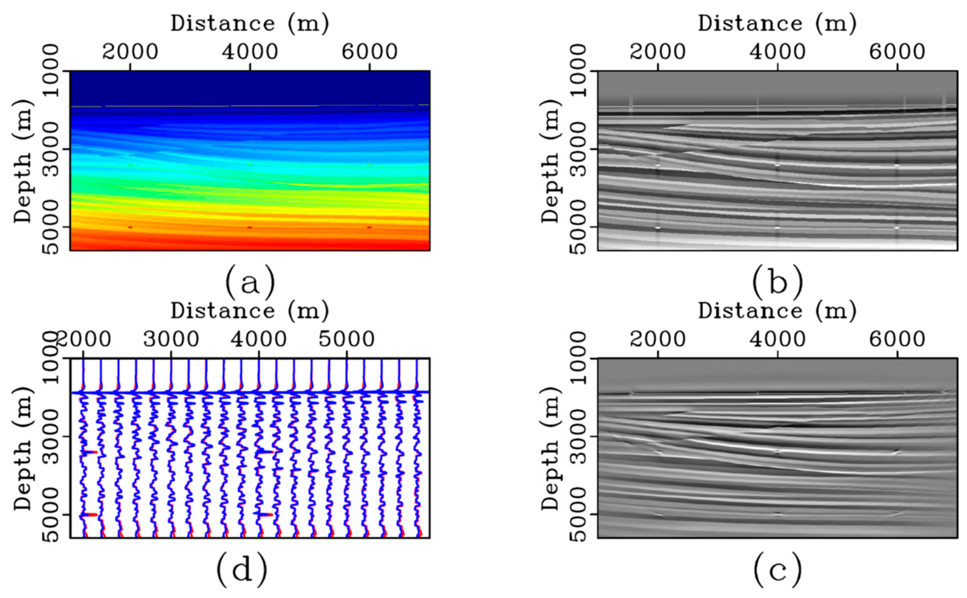
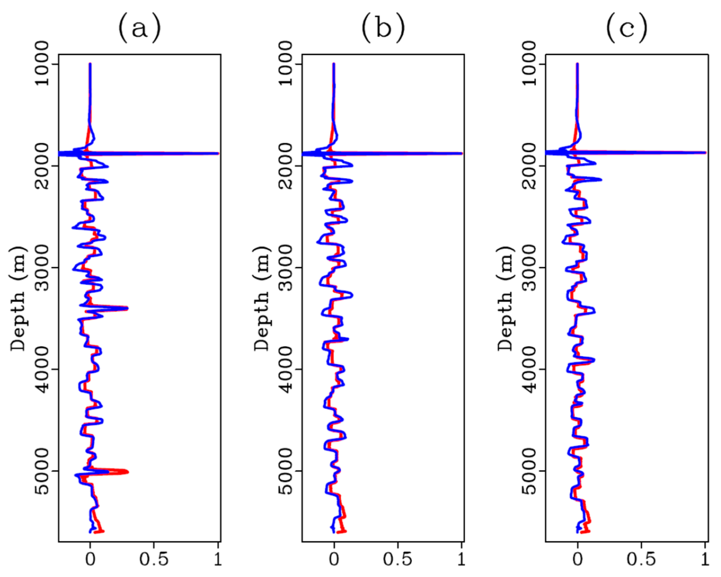
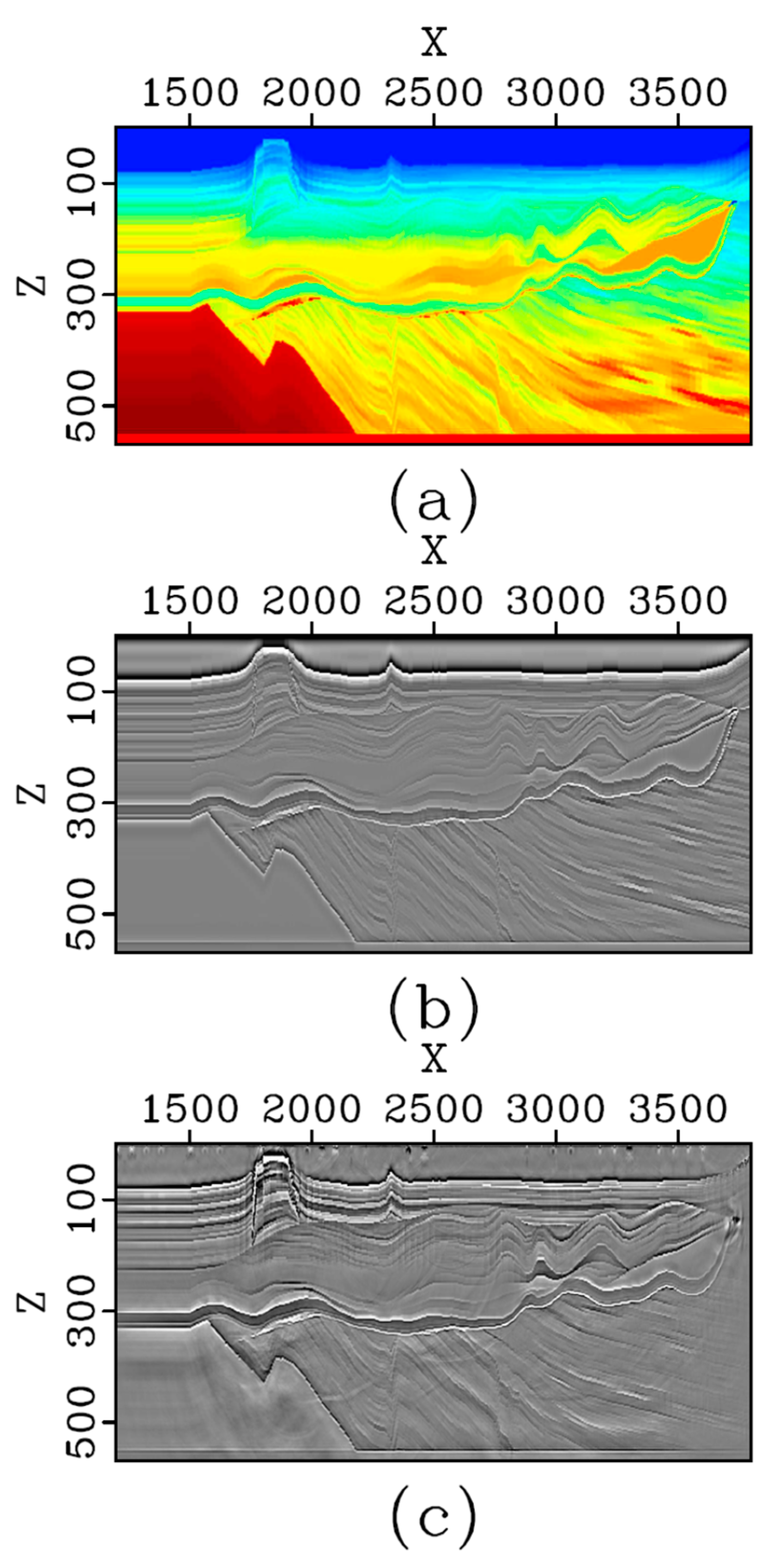
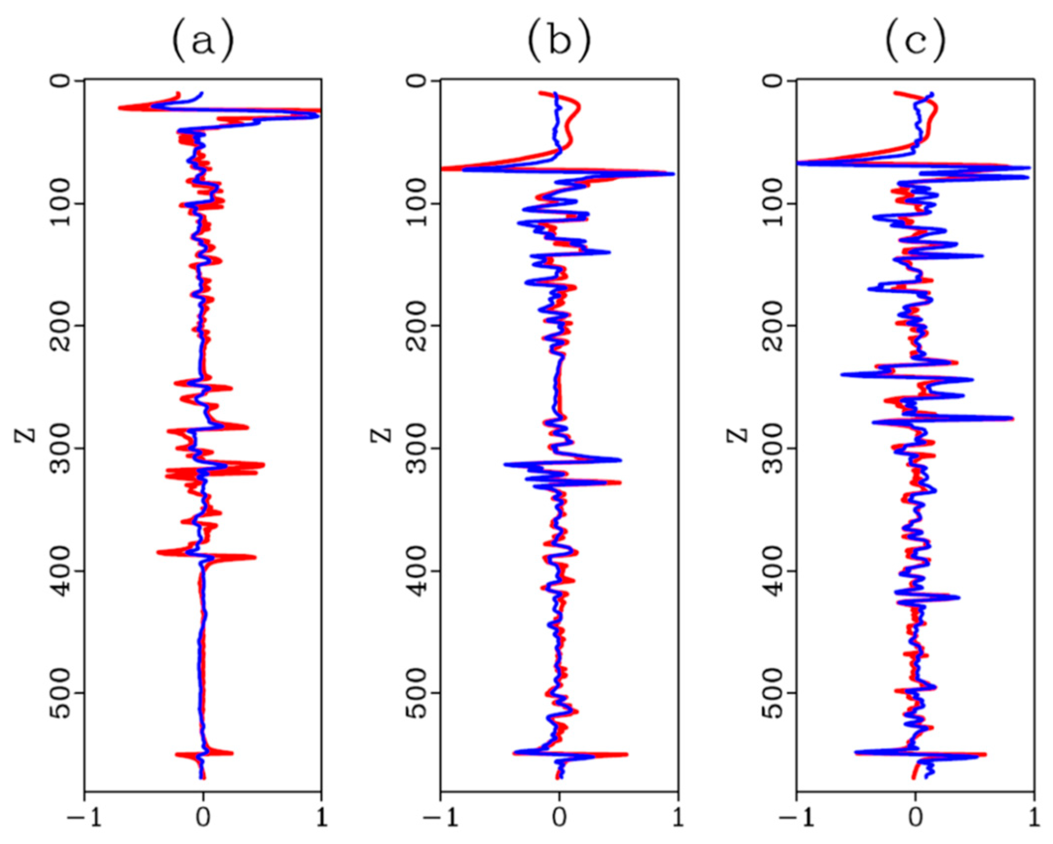
3. Numerical Examples

In this section, we demonstrate the effectiveness of the proposed imaging condition for the impedance perturbation estimation (Equation (14)) on synthetic data. The first example was designed to demonstrate the effectiveness of the proposed method on a laterally invariant model with uncorrelated velocity and density. Figure 4a and Figure 4b show the velocity and density model, respectively. Figure 4c shows the true relative impedance perturbation. We used the velocity and density in the first layer as the background velocity and density, respectively. We first subtracted the background impedance from the exact impedance and then analytically calculated the relative impedance perturbation. Figure 5a and Figure 5b show the filtered true velocity and impedance perturbation, respectively. Figure 5c illustrates the impedance perturbation estimated by our proposed method, which matches well with the true results. Note that the depth errors in the estimated acoustic impedance are due to the fact that we used a constant migration velocity.

Next, we demonstrated the acoustic impedance estimation on the Sigsbee2b model [17], and focused on the sediment areas with fine impedance structure. We performed acoustic finite difference modeling for synthetic data generation using a broadband source wavelet (${[f}_1,f_2{,f}_3{,f}_4]$= [0, 2, 56, 60] Hz). The exact velocity model is shown in Figure 6a, from which the density model was generated using a predefined relationship of the two parameters. A $V\left(z\right)$ velocity model and a constant density model were used for migration. We analytically calculated the exact impedance perturbation and applied the band-pass filtering to the exact result according to the bandwidth of input data. The filtered true impedance perturbation is shown in Figure 6b. In comparison, Figure 6c illustrates the impedance perturbation results estimated by our proposed method. Figure 6d displays the overlay of the two images (Figure 6b,c). The detailed comparison between Figure 6b,c at the three different locations are shown in Figure 7. An amplitude calibration was performed using reflections from the water bottom. In Figure 7, the filtered true impedance perturbation is shown in red and the estimated impedance perturbation is shown in blue. The numerical results demonstrate the overall good match between the estimated and the true impedance perturbation.

In the third example, we demonstrated the proposed method on a 2D transition zone model. The exact velocity model (labels show grid numbers) is illustrated in Figure 8a, and the density model had similar structural characteristics (not shown here). As in the previous example, synthetic data were generated using a broadband source wavelet. A smoothed version of the true velocity was used for migration, with the assumption of a constant density. Figure 8b shows the filtered true impedance perturbation, while Figure 8c illustrates the estimated results using the proposed method. Detailed trace comparisons between the two are shown in Figure 9 at the three different horizontal locations ($X=1900$, 2200, 3000). Figure 9b (at $X=2200$) and Figure 9c (at $X=3000$) show a slightly better match than Figure 9a ($X=1900$, inside the island) due to better illumination. The comparison shows the true and the estimated results match quite well, demonstrating the effectiveness of our method on complex models.

4. Discussion

In Equation (11b), we can see that the summation of the time derivative and the spatial gradient images had an extra term of ${\mathrm{c}\mathrm{o}\mathrm{s}}^2\theta$ compared to the time derivative image. When we designed the small-angle imaging condition in Equation (13), we mentioned that the exponential term approximated to $e^{-\alpha {\mathrm{s}\mathrm{i}\mathrm{n}}^2\theta }$. Since this exponential weighting was applied at each time step, we can consider the proposed imaging condition as the time derivative imaging condition weighted by the term ${\mathrm{c}\mathrm{o}\mathrm{s}}^2\theta e^{-\alpha {\mathrm{s}\mathrm{i}\mathrm{n}}^2\theta }$. Figure 10 shows the analysis of this term by choosing different parameter $\alpha$, compared to the term ${\mathrm{c}\mathrm{o}\mathrm{s}}^2\theta$. In the figure, we can see that a larger $\alpha$ attenuated the large reflections more rapidly than a small $\alpha$; on the other hand, the attenuation curve was smoother for a small $\alpha ,$ which generated less artifacts than a large $\alpha$. In all our examples in the previous section, we empirically chose $\alpha =5$ based on a compromise between the preservation of accuracy, and artifacts reduction. Figure 11 shows the sensitivity analysis of the inversion results using different $\alpha$ ($\alpha =0,5,10,20$) for the layered model (Figure 4). In the figure, we can see that for $\alpha =0,$ the velocity and impedance perturbation cannot be distinguished, while for a larger $\alpha$ ($\alpha =10$ and $\alpha =20$), the shallow part is problematic. In future studies, we may consider the functions of different forms to attenuate large reflections while still preserving the imaging quality.

In all our numerical examples, broadband sources were used for synthetic data generation. Broad bandwidth played an important role in seismic inversion. Increasing the bandwidth at the high-frequency end improved seismic resolution, and adding more low frequencies in the data reduced the side lobes of the seismic wavelet [18]. Figure 12 demonstrates the impact of low frequencies on the inversion result. For the Sigsbee2b model, we applied a band-pass filter ($f_1$ = 3 Hz, $f_2$ = 5 Hz, $f_3$ = 56 Hz, $f_4$ = 60 Hz) to remove low frequencies in the input data, and then estimated the impedance perturbation using our proposed method. The estimated impedance perturbations with and without low frequencies are shown in Figure 12a and Figure 12b, respectively. Figure 12a is the same as Figure 6c, and is repeated here for comparison. Figure 12c shows the trace comparison of Figure 12a,b at the horizontal location of 3500 m. The results demonstrate that low frequencies in the data affect the long-wavelength structures in the image. Low frequencies are crucial for both velocity and impedance inversions [8], and retaining low frequencies in the recorded data depends on broadband seismic acquisition and data processing.

As in conventional RTM, the proposed method assumes primaries only in the data, so de-multiple is a necessary preprocessing step in the case of strong multiples in the data. Even though our method was derived from the framework of amplitude-preserving RTM, the inversion was based on the Born approximation (Equation (4)). Therefore, transmission losses due to the overburden effects were also a challenge for our proposed method. The proposed method could be extended to finite-frequency based inversion [19] or FWI approaches [20] in the future work.

5. Conclusions

We proposed a weighted inverse scattering imaging condition for common-shot RTM, which outputs an estimation of the relative impedance perturbation. The construction of the weighting function was based on the two separate images from the conventional inverse scattering imaging condition. The proposed imaging condition was designed to select near-angle reflections during imaging, and therefore can separate the effect of impedance perturbation from velocity perturbation, for acoustic cases with variable velocities and densities. We demonstrated the effectiveness of the modified inverse scattering imaging condition using synthetic examples and showed that our method can produce reliable estimations of impedance perturbations.

References

1. Latimer, R.; Davidson, R.; van Riel, P. An interpreter’s guide to understanding and working with seismic-derived acoustic impedance data. Lead. Edge 2000, 19, 242–256. [Google Scholar] [CrossRef]
2. Routh, P.; Neelamani, R.; Lu, R.; Lazaratos, S.; Braaksma, H.; Hughes, S.; Saltzer, R.; Stewart, J.; Naidu, K.; Averill, H.; et al. Impact of high-resolution FWI in the Western Black Sea: Revealing overburden and reservoir complexity. Lead. Edge 2017, 36, 60–66. [Google Scholar] [CrossRef]
3. Barclay, F.; Bruun, A.; Rasmussen, K.B.; Alfaro, J.C.; Cooke, A.; Cooke, D.; Salter, D.; Godfrey, R.; Lowden, D.; McHugo, S.; et al. Seismic inversion: Reading between the lines. Oilfield Rev. 2008, 1, 42–63. [Google Scholar]
4. Beylkin, G. Imaging of discontinutes in the inverse scattering problem by inversion of a causal generalized Radon transform. J. Math. Phys. 1985, 26, 99–108. [Google Scholar] [CrossRef]
5. Jin, S.; Madariaga, R.; Virieux, J.; Lambaré, G. Two-dimensional asymptotic iterative elastic inversion. Geophys. J. Int. 1992, 108, 575–588. [Google Scholar] [CrossRef]
6. Forgues, E.; Lambaré, G. Parameterization study for acoustic and elastic ray+Born inversion. J. Seism. Explor. 1997, 6, 253–277. [Google Scholar]
7. Thierry, P.; Operto, S.; Lambare, B. Fast 2-d ray+born migration/inversion in complex media. Geophysics 1999, 64, 162–181. [Google Scholar] [CrossRef]
8. Bleistein, N.; Cohen, J.K.; Stockwell, J.W. Mathematics of Multidimensional Seismic Imaging, Migration, and Inversion; Springer: New York, NY, USA, 2001. [Google Scholar]
9. Bleistein, N.; Zhang, Y.; Zhang, G.; Gray, S.H. Migration inversion: Think image point coordinates, process in acquisition surface coordinates. Inverse Probl. 2005, 21, 1715–1744. [Google Scholar] [CrossRef]
10. Zhang, Y.; Ratcliffe, A.; Roberts, G.; Duan, L. Amplitude-preserving reverse time migration: From reflectivity to velocity and impedance inversion. Geophysics 2014, 79, S271–S283. [Google Scholar] [CrossRef]
11. Whitmore, N.D.; Crawley, S. Applications of RTM inverse scattering imaging conditions. In Proceedings of the 82nd Annual International Meeting, SEG, Expanded Abstracts, Las Vegas, NV, USA, 4–9 November 2012; pp. 1–6. [Google Scholar] [CrossRef]
12. Zhang, Y.; Xu, S.; Bleistein, N.; Zhang, G. True-amplitude, angle-domain, common-image gathers from one-way wave-equation migrations. Geophysics 2007, 72, S49–S58. [Google Scholar] [CrossRef]
13. Kiyashchenko, D.; Plessix, R.; Kashtan, B.; Troyan, V. A modified imaging principle for true-amplitude wave-equation migration. Geophys. J. Int. 2007, 168, 1093–1104. [Google Scholar] [CrossRef]
14. Liang, H.; Zhang, H. Wavelet-domain reverse time migration image enhancement using inversion-based imaging condition. Geophysics 2019, 84, S401–S409. [Google Scholar] [CrossRef]
15. Liang, H.; Zhang, H.; Liu, H. Reverse time migration for acoustic impedance inversion using inversion-based imaging condition. In Proceedings of the 89th Annual International Meeting, SEG, Expanded Abstracts, San Antonio, TX, USA, 15–20 September 2019; pp. 4365–4369. [Google Scholar] [CrossRef]
16. Rocha, D.; Tanushev, N.; Sava, P. Acoustic wavefield imaging using the energy norm. Geophysics 2016, 81, S151–S163. [Google Scholar] [CrossRef]
17. Paffenholz, J.; McLain, B.; Zaske, J.; Keliher, P. Subsalt multiple attenuation and imaging: Observations from the Sigsbee2B synthetic dataset. In Proceedings of the 72nd Annual International Meeting, SEG, Expanded Abstracts, Salt Lake City, UT, USA, 6–11 October 2012; pp. 2122–2125. [Google Scholar] [CrossRef]
18. Fons ten Kroode, F.; Bergler, S.; Corsten, C.; de Maag, J.W.; Strijbos, F.; Tijhof, H. Broadband seismic data—The importance of low frequencies. Geophysics 2013, 78, WA3–WA14. [Google Scholar] [CrossRef]
19. Zhang, H.; Liang, H.; Baek, H.; Zhao, Y. Computational aspects of finite-frequency traveltime inversion kernels. Geophysics 2021, 86, R109–R128. [Google Scholar] [CrossRef]
20. Qin, B.; Lambare, G. Joint inversion of velocity and density in preserved-amplitude full-waveform inversion. In Proceedings of the 86th Annual International Meeting, SEG, Expanded Abstracts, Dallas, TX, USA, 16–21 October 2016; pp. 1325–1330. [Google Scholar] [CrossRef]
21. Fomel, S.; Sava, P.; Vlad, I.; Liu, Y.; Bashkardin, V. Madagascar: Open-source software project for multidimensional data analysis and reproducible computational experiments. J. Open Res. Softw. 2013, 1, e8. [Google Scholar]
22. Bleistein, N. On the imaging of reflectors in the earth. Geophysics 1987, 52, 1426–1436. [Google Scholar] [CrossRef]
Figure 1. Workflow of the proposed method.
Applsci 13 05291 g001
Figure 2. Imaging results of a single trace (offset = 4000 m) showing (a) I d t ; (b) I d t + I ; and (c) I s m a l l   a n g l e ; Imaging results of a single trace (offset = 0 m) showing (d) I d t ; (e) I d t + I ; and (f) I s m a l l   a n g l e .
Applsci 13 05291 g002
Figure 3. Comparison of imaging results of a single trace (offset = 0 m) (a) using Equation (13) and (b) using Equation (14).
Applsci 13 05291 g003
Figure 4. (a) Velocity model; (b) density model; and (c) true relative impedance perturbation.
Applsci 13 05291 g004
Figure 5. (a) Filtered true relative velocity perturbation; (b) filtered true relative impedance perturbation; and (c) estimated relative impedance perturbation.
Applsci 13 05291 g005
Figure 6. (a) Velocity model for synthetic data generation; (b) filtered true impedance perturbation; (c) impedance perturbation estimated by the proposed method; and (d) overlay plot of the two images (red: true, blue: estimated).
Applsci 13 05291 g006
Figure 7. Comparison of filtered true impedance perturbation (red) and estimated results (blue) at three horizontal locations: 2000 m (a); 3500 m (b); and 5000 m (c).
Applsci 13 05291 g007
Figure 8. (a) A 2D transition zone velocity model; (b) true relative impedance perturbation after band-pass filtering; and (c) estimated relative impedance perturbation computed using the proposed method.
Applsci 13 05291 g008
Figure 9. Comparison of filtered true impedance perturbation (red) and estimated results (blue) at three locations: (a) X = 1900; (b) X = 2200; and (c) X = 3000.
Applsci 13 05291 g009
Figure 10. Analysis of different angle-dependent functions.
Applsci 13 05291 g010
Figure 11. Estimated relative impedance perturbation for the layered model using different α in the weighting function in Equation (14): (a) α = 0 ; (b) α = 5 ; (c) α = 10 ; and (d) α = 20 .
Applsci 13 05291 g011
Figure 12. Comparison of estimated impedance perturbation with (a) and without (b) low frequencies in input data. (c) Trace comparison of estimated impedance perturbation with (blue) and without (green) low frequencies at the horizontal location of 3500 m.
Applsci 13 05291 g012
Disclaimer/Publisher’s Note: The statements, opinions and data contained in all publications are solely those of the individual author(s) and contributor(s) and not of MDPI and/or the editor(s). MDPI and/or the editor(s) disclaim responsibility for any injury to people or property resulting from any ideas, methods, instructions or products referred to in the content.