Article

On-Orbit Magnetometer Data Calibration Using Genetic Algorithm and Interchangeability of the Calibration Parameters

Laboratory of Lean Satellite Enterprises and In-Orbit Experiments (LaSEINE), Kyushu Institute of Technology, Kitakyushu 804-8550, Japan
*
Author to whom correspondence should be addressed.
Submission received: 28 April 2023 / Revised: 25 May 2023 / Accepted: 29 May 2023 / Published: 1 June 2023
(This article belongs to the Special Issue Small Satellites Missions and Applications)

Abstract

:
Magnetometers are important sensors with applications in the attitude determination and control systems of satellites. CubeSats have certain limitations related to power, mass, and volume. Due to this, CubeSat magnetometers are not separated from other electrical circuits inside the satellite. Thus, it is important to calibrate the magnetometer, simulating operating conditions while the satellite is running before the launch. However, due to the limited facilities, not every CubeSat is able to calibrate its magnetometers properly on the ground. This study focuses on the calibration of on-orbit magnetometer data observed by BIRDS-3 CubeSats with a genetic algorithm. High oscillations in the total magnetic field were found in the on-orbit magnetic field data measured by magnetometers inside BIRDS-3 CubeSats. Nine unknowns, scaling factors, non-orthogonal angles, and offsets are identified with the genetic algorithm. This paper discusses the factors that affect the high oscillations in the measured total magnetic field data. For the calibration, we used magnetic field data similar to those of a model magnetic field, as the deviation is smaller. This paper presents the accuracy of determining unknowns using the genetic algorithm, as well as the interchangeability of the answers with additional orbit data from the same satellite. This method can be used in the future to calibrate magnetometers inside CubeSats before or after launch.

1. Introduction

The attitude determination and control system (ADCS) is a subsystem in satellites. Magnetometers are sensors commonly used in the ADCS. If the magnetometer data are not calibrated properly, using simulations of on-orbit operating conditions with the running satellite, these data can be affected by residual magnetic fields. CubeSats have limited volume, space, and power. Due to the limitations of CubeSats, their magnetometers are not separated from other electrical circuits installed inside the satellite. Incorrect magnetometer data can lead to malfunction of the attitude determination and control system. However, not every CubeSat developer has the facilities to calibrate the magnetometers precisely. Therefore, not every CubeSat is able to calibrate its magnetometers correctly before flight.
Magnetometers can provide unexpected results due to scaling factors, offsets, and non-orthogonality errors. Due to the residual magnetic field inside the satellite, the magnetometers require an additional calibration. That is, despite being calibrated by the ground test, magnetometers need to be calibrated again with on-orbit data.
Previous studies have demonstrated calibration methods to calibrate on-orbit magnetometer data. Bangert et al. [1] described the performance characteristics of the UWE-3 pico-satellite’s attitude determination and control system. According to the on-orbit results, attitude estimation was not accurate. It was found that the magnetometer data were not calibrated properly. Oscillations in total magnetic field, |B|, were identified. Bangert’s study attempted to calibrate the on-orbit magnetometer data and set the correct parameters using standard minimization algorithms. Gain, cross-axis effects, and offsets were considered in the calibration method. A study presented by Foster [2] shows an extension of the two-step estimation algorithm to calibrate solid-state strap-down magnetometers. Additionally, the authors stated that this algorithm can be applied to any two- or three-axis sensor. This method was not tested for magnetometers installed in a whole vehicle or spacecraft. Pourtakdoust et al. [3] presented the calibration of magnetometers using the hyper least square (HyperLS) method. This method was tested with a Honeywell HMC5883L magnetometer. The authors mentioned that magnetometer outputs were affected by various disturbances due to manufacturing faults and limits as well as environmental impacts, requiring calibration for meaningful application. The authors defined the errors as hard iron errors, soft iron errors, bias, scale factors, and misalignment in their study. Wang et al. presented a calibration method utilizing a back propagation (BP) neural network [4]. The trained BP neural network is able to predict the true magnetic field, referring to the observational data. This method provided an error of less than 10 nT. The authors trained the network with the Levenberg–Marquardt (LMBP) algorithm, considering the non-orthogonal error, measurement noise, and constant drift. This calibration method is verified by a simulation. Previous studies used the genetic algorithm to calibrate magnetometers. Xueliang et al. [5] presented a calibration method for a three-axis magnetometer using the genetic algorithm. In this study, three-axis non-orthogonal error, sensitivity error, and the residual magnetic effect are considered. This method was tested by numerical simulation and experimentation using a fluxgate magnetometer. The author mentioned that it is difficult to achieve high accuracy with methods such as the least square method for model parameter estimation. In our study, we used on-orbit data collected by three satellites, with the evaluation function as the error (defined as in Equation (5) shown in the methodology). Moreover, we focused on low-latitude regions where the deviation of the true magnetic field from a model magnetic field is expected to be small and applied the genetic algorithm.
Chekhov et al. [6] also presented magnetometer calibration with the genetic algorithm for industrial micro-controllers. Remotely operated underwater vehicles use attitude and heading reference systems (AHRSs). AHRSs use magnetometer and accelerometer data to determine the heading of a vehicle. For genetic algorithm calibration, bias errors, gain errors, and misalignment errors were considered. This method was verified with simulated and collected magnetometer data. It is shown that the genetic algorithm shows an improvement over the recursive least square method after testing on a mission. Most research has attempted to use two-step estimation [2], standard minimization [1], the hyper least square method, strict ellipsoid, and the three-step method [3]. However, in every case, the magnetometer calibration conditions are different. The majority of previous authors have used error models. The accuracy of calibration depends on the true magnetic field or the model used. Xuelinag and Chekhov stated that the genetic algorithm shows an improvement in magnetometer calibration.
Genetic algorithms have been applied to many areas successfully [7] (p. 3). Genetic algorithms are suitable for solving problems unable to be solved easily using classical methods such as least square methods [6,7,8]. Genetic algorithms are known as effective candidates for parameter selection for non-linear, non-continuous problems wherein a large number of unknown parameters must be found while local maxima can exist in the search domain. In order to observe the performance, we used the genetic algorithm for magnetometer calibration.
The purpose of the paper is to use a genetic algorithm to calibrate the on-orbit magnetometer data collected by CubeSats. Our study focuses on calibrating on-orbit magnetometer data using the genetic algorithm. This method is tested with magnetometer data observed by BIRDS-3 CubeSats. This study discusses the accuracy and interchangeability of the answers found using the genetic algorithm for selected regions. Even though there remain limitations, this study demonstrates the level of calibration accuracy that can be achieved using the genetic algorithm for magnetometers installed in CubeSats.
The novelty of the present work concerns applying the genetic algorithm to low-latitude regions (where the true magnetic field is expected to be similar to a model magnetic field) of on-orbit magnetometer data and checking the interchangeability of the parameters with other on-orbit data measured from the same satellite. Moreover, this work considers the reasons for the high oscillations seen in the total magnetic field measured on orbit.
The present work can contribute to calibrating the on-orbit magnetometer data collected by CubeSats, aiding CubeSat developers in overcoming limitations when calibrating magnetometers.
This paper consists of six sections. Section 1 is the introduction; Section 2 describes the materials; Section 3 describes the methodology used in this study; Section 4 describes the results obtained using the aforementioned methodology; Section 5 is the discussion; and Section 6 is the conclusion.

2. Materials

BIRDS-3 is the third project of the BIRDS program [9]. BIRDS-3 is a constellation of three CubeSats deployed to orbit on 17 June 2019 [10]. 
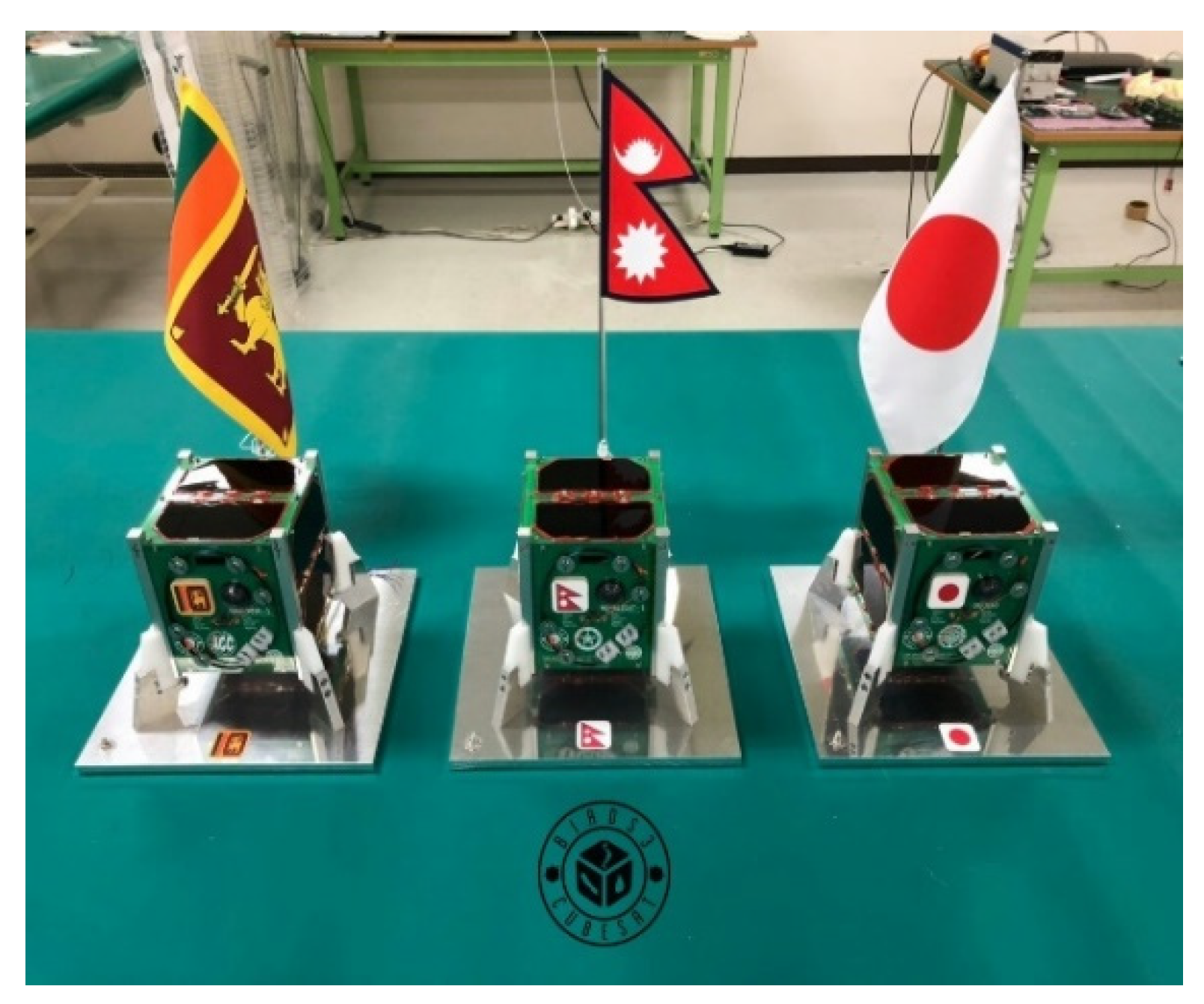
Figure 1 shows the BIRDS-3 flight models. The external dimensions and weight of each BIRDS-3 CubeSat are 113.5 mm × 100 mm × 100 mm and 1.05 kg, respectively. All three satellites re-entered the atmosphere on October 2021.
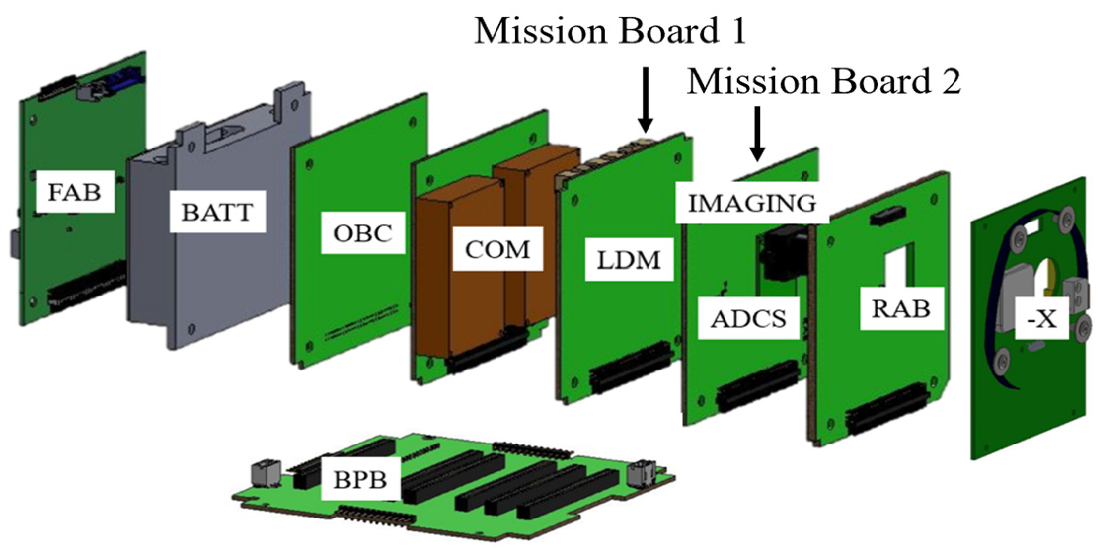
The BIRDS-3 CubeSats had four missions, namely the Imaging Mission (CAM), the LoRa Demonstration Mission (LDM), the Attitude Determination and Control System (ADCS), and the Software Configurable Backplane Mission (BPB):BIRDS-3 FM CPLD. The BIRDS-3 CubeSats had two mission boards named Mission Board 1 and Mission Board 2. ADCS and CAM were installed on Mission Board 2. BIRDS-3 satellites have three-axis magnetic torquers for ADCS and were implemented in printed circuit boards in order to save space. The magnetometer was installed in Mission Board 2 in the ADCS section. 
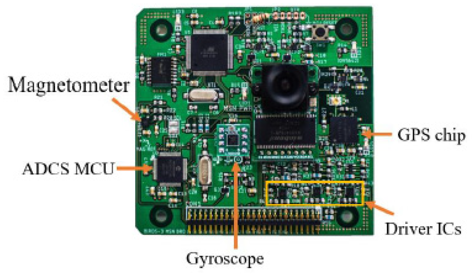
Figure 2 shows the location of Mission Board 2 (ADCS mission board), and Figure 3 shows the location of the magnetometer. The MMC5883MA magnetometer was used in BIRDS-3 CubeSats.
On-orbit magnetometer data were used as part of the BIRDS-3 attitude stabilization system. B-dot control was used to stabilize the CubeSats. The B-dot algorithm [11] is a simple algorithm used to reduce the angular velocity of satellites. It requires the rate of changes in magnetic field flux density, measured by magnetometers. Magnetometer data were the key input of the B-dot algorithm. The attitude stabilization system of BIRDS-3 failed in orbit. It was found that the on-orbit magnetic field data observed by all three magnetometers were different from the expected results when compared to magnetic field models such as the World Magnetic Model (WMM) [12]. Before the flight, a magnetometer calibration test using a Helmholtz coil was conducted on the ground utilizing an engineering model of the magnetometer. This calibration test was performed only for the magnetometer. The whole satellite was not used to calibrate the magnetometer. Moreover, the gain and non-orthogonality angles were not estimated before the flight. 
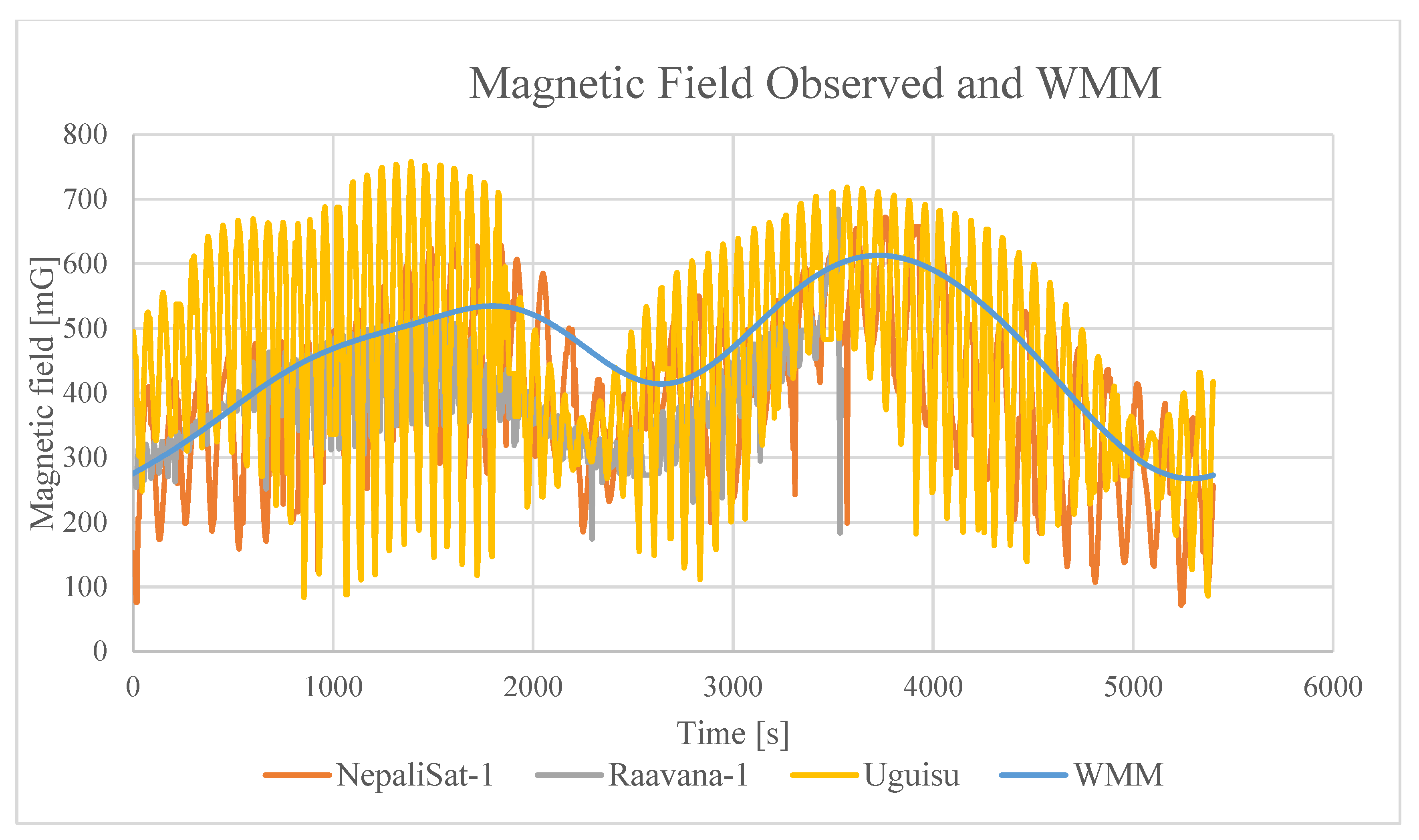
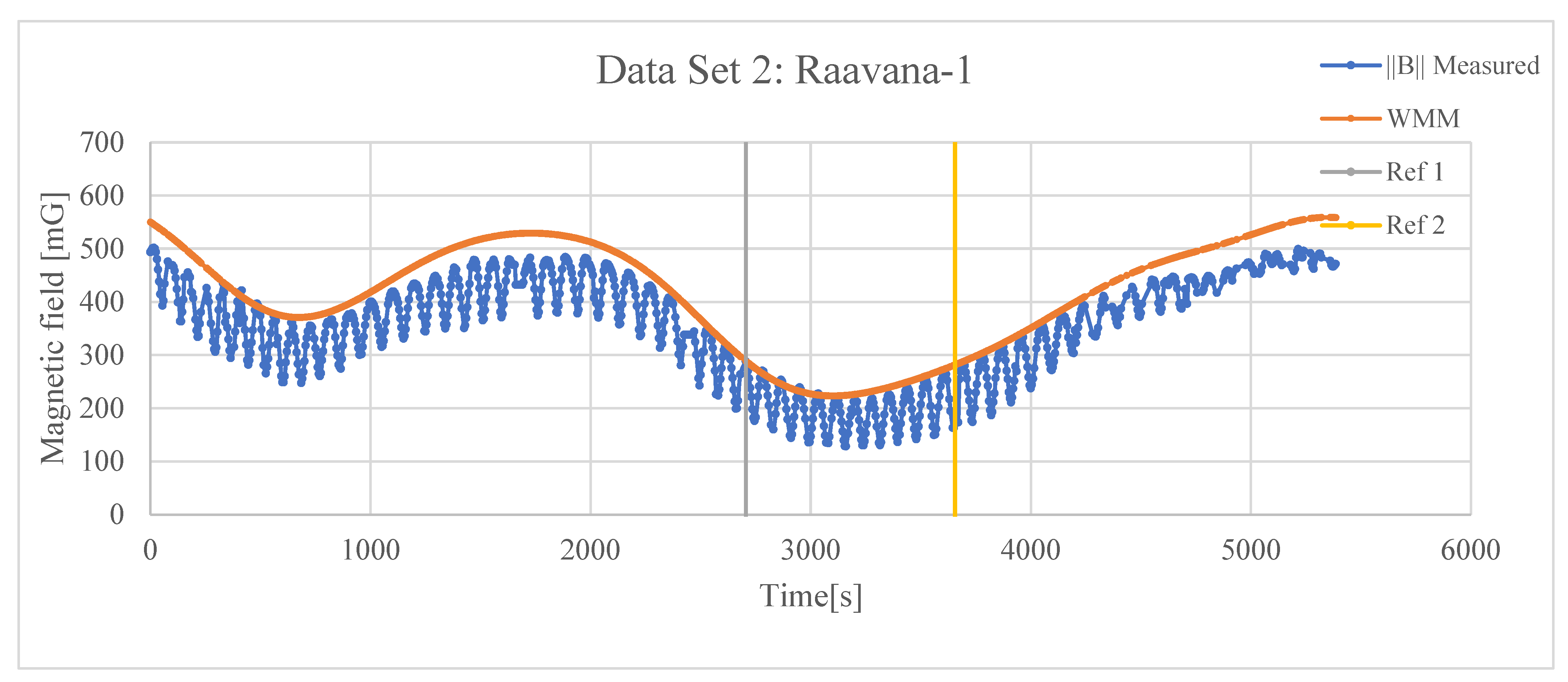
Figure 4 shows the on-orbit magnetometer data observed by BIRDS-3 CubeSats after their deployment from the International Space Station. The BIRDS-3 CubeSats were deployed into orbit at 7:15 p.m. (JST) on 17 June 2019. The data were collected after 16 s of deployment. The zero in the time axis corresponds to the 16 s after the deployment. Latitude at deployment was approximately 1.433 degrees north, and longitude was −57.903 degrees.
In Figure 4, the magnetometer data are compared with the WMM. The orange line indicates the magnetometer data of NepaliSat-1, the gray line indicates the magnetometer data of Raavana-1, the yellow line indicates the magnetometer data of Uguisu, and the blue line indicates the WMM. Figure 4 shows the difference between observed and WMM magnetic fields. There are heavy variations in the observed total magnetic field measured in all three satellites due to the offsets, gains, and non-orthogonal angles in the magnetometers. These errors in the magnetometer data must be corrected.

3. Methodology

3.1. Ground Testing

Before launch, the residual magnetic field of the satellite was not tested. As the magnetic field measured by the magnetometers had high oscillations during orbit, we decided to measure the residual magnetic field of the satellite. This test was conducted within the magnetic shield chamber belonging to ISAS/JAXA (Institute of Space and Astronautical Science/Japan Aerospace Exploration Agency) located in Sagamihara, Japan. It is challenging to perform this experiment in a normal environment, due to the Earth’s magnetic field as well as disturbance magnetic fields. Therefore, the experiment was conducted in the magnetic shield room. Figure 5 shows the test setup.
Different operation modes were provided as input to the Birds-3 FM (Flight Model) backup, and magnetometer readings inside the CubeSats were checked, the difference between the FM and the FM backup being that no solar cells were attached to the FM backup. Normal sampling (NS), high sampling (HS), and ADCS modes were executed. The normal-sampling mode was the nominal mode of the CubeSats. In high-sampling mode, the sensor data were collected every 5 s. The residual magnetic field after deducting the ambient magnetic field in the shield room was as follows: X: 16,570.8 nT (165.70 mG), Y: 1070.8 nT (10.70 mG), and Z: 2283.3 nT (22.83 mG).
We have mentioned three calibration parameters, namely offsets, non-orthogonality errors, and gains. Offsets are affected by residual magnetic fields. Non-orthogonal errors are due to manufacturing errors. Gains are treated as the sensitivity of the magnetometer. Among the parameters, only the offset values are affected due to the residual magnetic field inside the satellite.
Figure 6 shows the experimental results. Blue indicates the X-axis of the magnetometer; orange indicates the Y-axis of the magnetometer; and gray indicates the Z-axis of the magnetometer.

3.2. Calibration Method

The genetic algorithm (GA) has been proven to be better in complex finding problems [7]. The genetic algorithm is an algorithm based on natural selection and reproduction [13]. Genetic algorithms can be used to find the best solution to a given problem. The main processes of the genetic algorithm are selection, crossover, and mutation. An initial population was defined in order to find solutions from the genetic algorithm.
The nine unknowns to be found in this study were the three offsets of x, y, and z, gains of a, b, and c, and non-orthogonality angles of λ, ρ, and ϕ. The unknowns are shown in Figure 7. Definitions of the angles are shown in Figure 8 [14]. The unknowns were defined as chromosomes or genes, as shown in Figure 7. One gene was represented by 12 bits.
The genetic algorithm requires a fitness function to find the best match for unknowns. The difference between the observed magnetic field and the model magnetic field was defined as the fitness function. The non-orthogonality angles of ρ, λ, and ϕ are shown in Figure 8. BreX, BreY, and BreZ axes are considered perfect orthogonal axes taken as calibrated values in Equations (1)–(3). Bx, By, and Bz are the non-orthogonal axes of the magnetometer sensors considered as measured values in Equations (1)–(3). ρ is the angle from the nominal Y axis to the X–Y plane. λ and ϕ are the angles from the nominal Z-axis to the X–Z and Z–Y planes, respectively. Equations (1)–(3) show the relationship between the calibrated magnetic field in each axis, the measured values, gain, and offsets, and the non-orthogonal angles.
B r e X = B x x / a
BreY = By - y - BreX   × sin ρ × b cos ρ × b
B r e Z = B z z B r e X × sin λ × c B r e Y × sin ϕ × cos λ × c c × cos ϕ × cos λ
B t 2 = B reX 2 + B reY 2 + B reZ 2
The genetic algorithm attempts to minimize the error between the total calibrated magnetic field and the WMM, which is considered to be the true solution. The RMS (root mean square) difference between track line data and the WMM was less than 200 nT [15] (p. 60). Thus, we believed this accuracy to be sufficient for us to use the WMM as the true solution. The calibrated total magnetic field Bt is shown in Equation (4). The error “e” is defined as Equation (5). Bwmm stands for the values taken from the WMM. In this equation, N denotes the number of data available.
e = Σ B w m m B t 2 B w m m N
The values used for the parameters in the genetic algorithm are shown in Table 1. The initial population was a set of randomly chosen solutions. In this study, we selected an initial population of 1000. The initial population can be thought of as a set of genes. The number of generations denotes how many generations are iterated to find the best solution. The software stops when the given number of generations is processed. We selected the number of generations as 100 in order to find the unknowns for this study. Next, we processed the initial population to find the most suitable answers for the unknowns. In the selection operation, we selected individuals from the current population. The selection operation allows the genes to pass to the next generation. Best genes are determined using the fitness function. A selection ratio of 0.3 was used in this study. Mutation is another genetic operator. Mutation can change a gene and create a new individual. The mutation ratio is the probability of altering the bits in genes. Successful mutations survive during this process. Precision of the gene is represented by the number of bits. In the genetic algorithm, the genes are represented in binary. In this study, one gene was represented by 12 bits, as mentioned in the previous section.
We focused on the data collected from low-latitude regions in which the true magnetic field is similar to the model magnetic field. Next, we applied the genetic algorithm to the selected region. After that, we checked the interchangeability of answers between other orbits. For the BIRDS-3 data, the World Magnetic Model was used as the true data. This method was applied to the on-orbit magnetometer data observed by BIRDS-3 CubeSats, and the results are presented in the next section. Please refer to the Supplementary Materials section for the magnetometer data observed by BIRDS-3.

4. Results

Accuracy of Interchangeability of Answers

We selected low-latitude regions to apply the genetic algorithm. This is because the deviation of the true magnetic field from the WMM is expected to be small. Next, the answers given by the genetic algorithm were applied to other available orbit data of the same satellite. This method was applied to the on-orbit magnetic field data from NepaliSat-1, Uguisu, and Raavana-1.
Figure 9 shows the data set used for calibration. The region between Ref 1 and Ref 2 was selected for GA application. The geographic latitude and magnetic latitude are shown in Figure 10. Table 2 shows the range of unknowns used for the GA. The nine parameters were searched to provide the best match with reference to the WMM values, and the calibrated values were calculated using the nine parameters.
Table 3 shows the parameters found by applying the GA to the selected region of Data Set 2 of Raavana-1, shown in Figure 9.
e m = Σ B w m m B m 2 B w m m N
e = Σ B w m m B t 2 B w m m N
Figure 11 shows the results of Data Set 2 collected by Raavana-1. First, the genetic algorithm was applied to the selected region, as shown in Figure 9. Next, the answers given by the genetic algorithm (Table 3) were applied to the whole orbit and to other available on-orbit data collection by the same satellite. Table 4 provides a summary of the error values before calibration, calculated according to Equation (6), and the error values after calibration according to Equation (7). In Equation (6), Bm denotes the measured total magnetic field; e m denotes the error value before calibration; and e denotes the error value after calibration in Equation (7). The third column of Table 4 shows the error value for the selected region between Ref 1 and Ref 2 in Figure 9. The fourth column shows the error value for all the data used in the data set.
Using the parameters shown in Table 3, i.e., the parameters found from Data Set 2, we calibrated the magnetometer data of a whole orbit, named Data Set 3. Data Set 2 comprises data collected on 14 February 2021 by Raavana-1. Data Set 3 comprises data collected again on 11 April 2021 by Raavana-1. Figure 12 shows the calibration results obtained in this way. The calibrated magnetic field matches well with the WMM model. The overall error is 0.03, as shown in the fifth column of Table 4, which is as good as 0.02 (the fourth column) of the error for the original data of Data Set 2. We repeated similar steps using Data Set 3. The result is shown in Table 5. The calibration parameters were derived by applying the genetic algorithm to Data Set 3. Then, the parameters were used to calibrate the measurement data of Data Set 2. The overall errors (0.03 and 0.07 in the fourth and fifth columns of Table 5) are not as good as those in Table 4. Therefore, we use the parameters in Table 3 as the calibration parameters of magnetometers onboard Raavana-1.
The results of the other two satellites’ (Uguisu and NepaliSat-1) magnetometer calibrations are shown below. First, the genetic algorithm was applied to the section of Data Set 2 shown between Ref 1 and Ref 2 in Figure 13, where the magnetic latitude is between −30.61 and 10.28 degrees for Uguisu. Next, the answers were applied to the whole of Data Set 3. The genetic algorithm was applied to the section shown in Figure 14, where the magnetic latitude is between 12.45 and −21.97 degrees for Nepalisat-1. Next, the answers were applied to Data Set 2.
Table 6 shows the parameters found by applying the GA to the data shown in Figure 13 and Figure 14 using the selected region shown in the figures. Using those parameters, we evaluated the error of other data sets obtained by the same satellites. The results are shown in Table 7 and Table 8.
According to the results shown above using the on-orbit magnetometer data of Raavana-1, Uguisu, and NepaliSat-1, it is proven that the genetic algorithm can be used to calibrate on-orbit magnetometer data, reducing discrepancies from the WMM.

5. Discussion

It is shown that our results for a selected region can be applied to other orbit data obtained by the same satellite. If the obtained nine parameters are correct, the calibrated result should match with the WMM regardless of when the measurement is performed, as long as the WMM is steady. WMM coefficients are estimated using data measured during magnetically quiet periods. The combined error of the WMM 2020 is 129 nT in the total magnetic field [15] (p. 67). In Table 9 below, we list the Kp-index of when the measurement was performed. From this table, we can say that the magnetic field was quiet, and the WMM is an adequate “solution” for the genetic algorithm.
Although the calibrated results obtained by parameters derived from an additional data set provided reduced error values, as shown in Table 4, Table 7 and Table 8, we still could not reduce the oscillation to the degree we desired. To determine the measured source of oscillation, we ran the GA simulation by dropping some of the parameters from the subject of the search. We applied the GA for specific low-latitude regions of each data set. In each simulation, only six parameters, instead of nine, were searched. Table 10 shows the results. In the table, without gain means that we searched only the offset (X, Y, and Z) and non-orthogonal angles (λ, ρ, ϕ) while fixing the gain values (a, b, c) to 1. The errors when gain and offsets were not considered were larger than the error when non-orthogonal angles were not considered. According to the results, the main reasons for the high oscillations are offsets and gain.
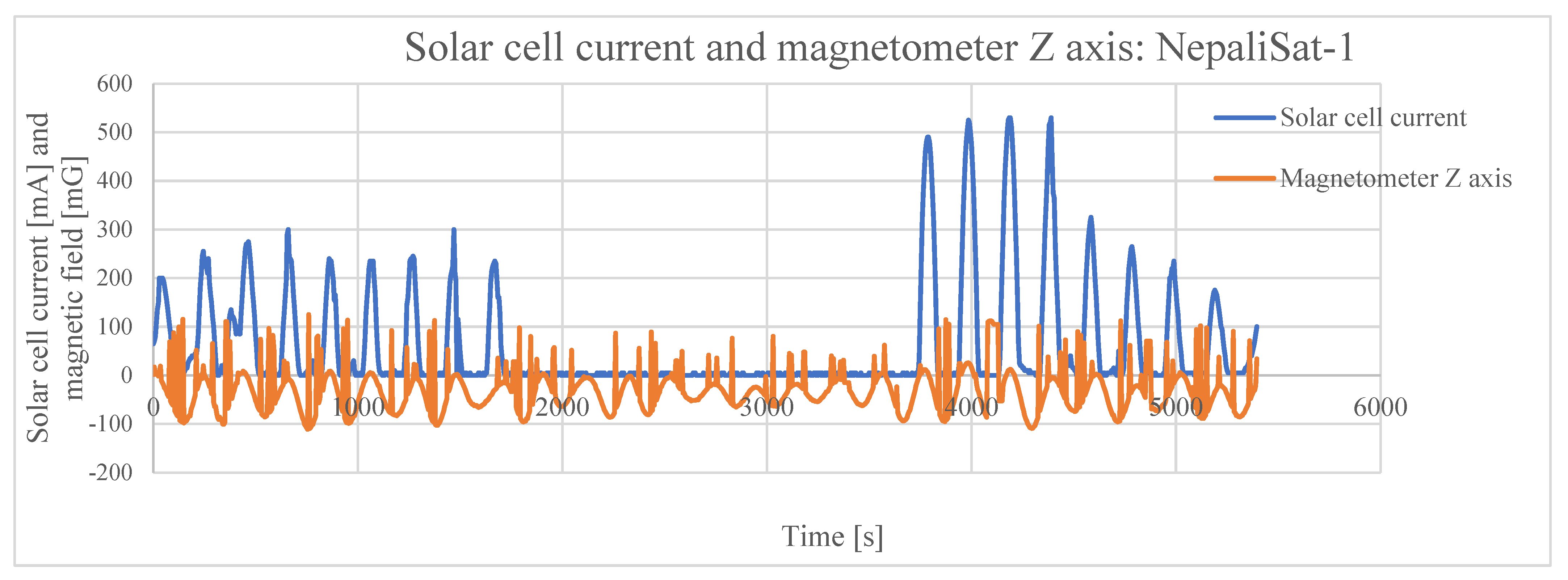
Next, the solar cell output pattern and the magnetometer output pattern for each axis were checked to confirm the reason for the high oscillations observed. The solar cell graph pattern and the magnetometer graph pattern have similar behavior, proving that each axis’ oscillation of magnetometers stems from the satellites’ rotation. One example is shown in Figure 15; the solar cell current is shown in mA, and the magnetic field is shown in mG. Each axis of the magnetometer data has an oscillation due to satellite rotation. However, we should not observe an oscillation in the total magnetic field. Therefore, the oscillation remaining after calibration is because the parameters obtained by GA are not yet perfectly matched.
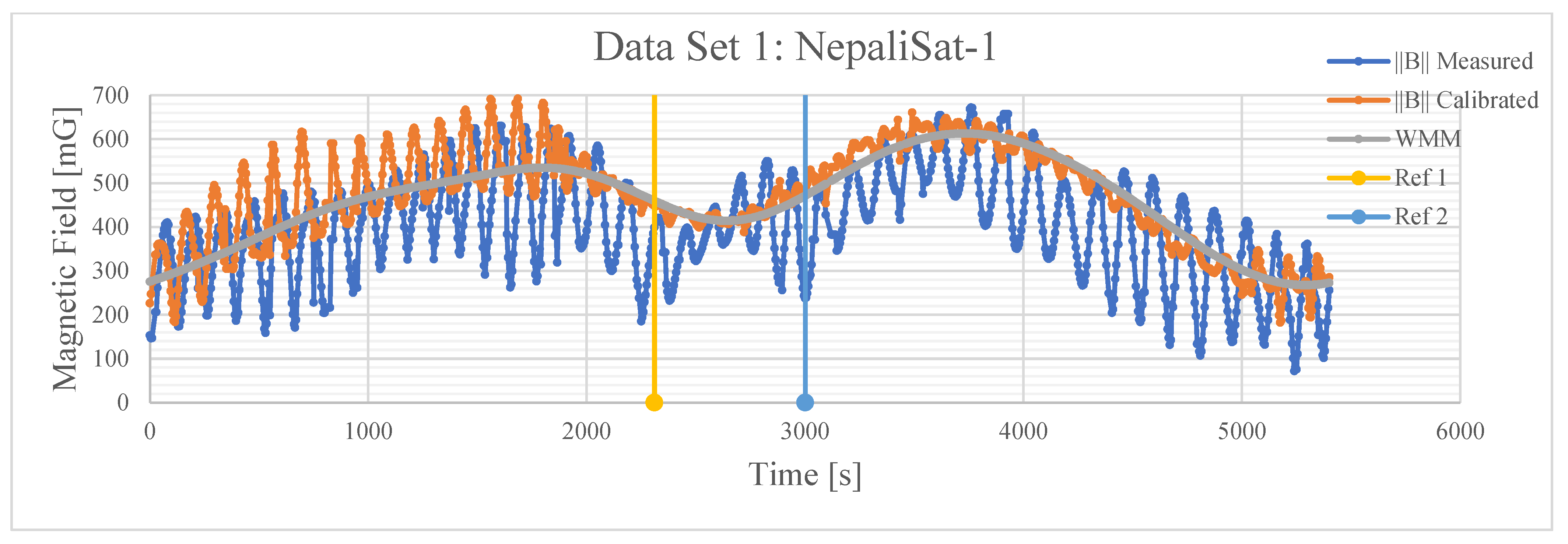
As we still observed high oscillations in the calibrated result, we attempted to use the frequency amplitude contained in the measured data to reduce the high oscillations. From Figure 15, we can see that the high-frequency oscillation is due to a combination of the satellite’s rotation and the mismatch of calibration parameters. From Figure 15, we determine the satellite rotates at about 0.005 Hz (1.8 deg/s). In Figure 16, we show the frequency spectrum of Data Set 1 of NepaliSat-1. It shows a peak at around 0.007 Hz. Instead of using the error defined in Equation (5) as the evaluation function of the GA, we used the sum of the magnitude of frequency amplitude and WMM data. The smaller the amplitude, the better the ranking is. In this search, we used the entire data sets of whole orbits rather than a selected region within low-latitude regions.
The following Equations (8)–(10) were used to apply genetic algorithms in this case. Equation (10) was used as the evaluation function. E1 and E2 were chosen to make e/E1 and e2/E2 both approximately one at the first generation.
  e = Σ B w m m B t 2 B w m m N
e 2 = Σ ( a m p l i t u d e   o f   f r e q u e n c y   s p e c t r u m )
e = e E 1 + e 2 E 2 / 2
Table 11 shows the parameters obtained from the GA. By comparing with Table 6, we can observe that the offset of the X-axis has been reduced. 
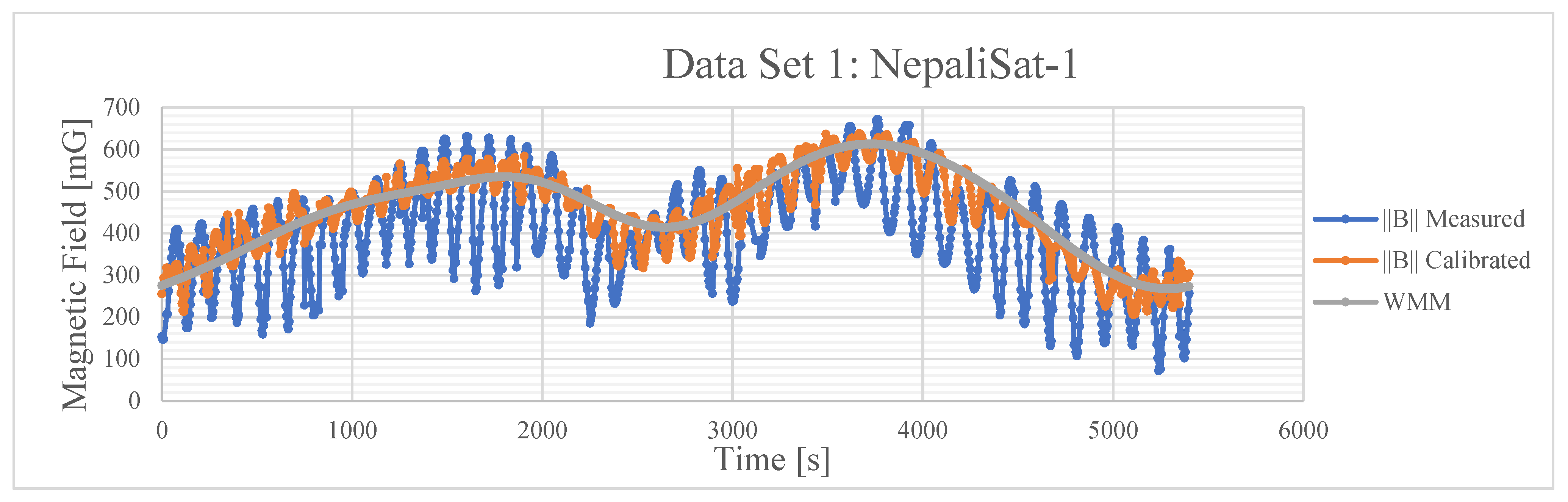
Figure 17 shows the calibrated result. Compared to Figure 14, we can see that the oscillations in the observation were reduced significantly in the first part of the graph, where we noticed high oscillations even after calibration with Equation (5).

6. Conclusions

CubeSats have limitations, as mentioned in the introduction section. Thus, magnetometers are not separated from electrical circuits inside the satellites. Therefore, magnetometers should be calibrated properly before flight. However, most CubeSat developers do not have the facilities to calibrate magnetometers with in-orbit conditions. Magnetometers are important sensors used in attitude determination and control systems. In this study, we investigated the magnetometer data collected by the BIRDS-3 CubeSats Raavana-1, NepaliSat-1, and Uguisu that flew with an orbit of 51.6-degree inclination and approximately 400 km altitude. There was a heavy variation in the magnetometer data collected when compared to a magnetic model.
The genetic algorithm was used in this study to calibrate the magnetometer data. We focused on non-orthogonality angles, offsets, and gains to calibrate the on-orbit magnetometer data. According to the results, applying the genetic algorithm to low-latitude regions and interchanging the answers with other available on-orbit data collected by the same satellite is possible. We defined the error as the difference from the WMM value, regarding the WMM value as a “true” solution. We use the error as the evaluation function of the genetic algorithm; the smaller, the better. According to the results, we could reduce the error with the genetic algorithm compared to the error in the measured magnetometer data. We were able to show that the high oscillations in the total magnetic field are mostly due to the gain and the offset. Next, we discussed using frequency amplitude in the genetic algorithm to reduce the oscillations. In this case, we defined two errors. One was the difference from the WMM value. The other was the oscillation amplitude of frequency, which was higher than expected due to satellite rotation. In this case, we used entire data sets of whole orbits. According to the results, we show that only using the difference from the WMM value for low-latitude data as the evaluation function gives better calibration results than using both the high-frequency oscillation and the difference from the WMM value as the evaluation function.
We tested the genetic algorithm for flight magnetometer data collected by three satellites and confirmed that the method is sufficient in calibrating on-orbit magnetometer data.
The calibration method outlined in this paper still has room for improvement. We could not remove the oscillations in the total magnetic field completely. Finding a better way to reduce oscillations remains a goal of future work.

Supplementary Materials

The following supporting information can be downloaded at Withanage, Dulani (2023), “On-orbit magnetometer data observed by BIRDS-3 CubeSats”, Mendeley Data, V1, doi: 10.17632/2b2rvxccyx.1, available online: https://data.mendeley.com/datasets/2b2rvxccyx/1, accessed on 27 April 2023.

Author Contributions

Conceptualization, D.C.W., M.T. and M.C.; methodology, D.C.W., M.T. and M.C.; software D.C.W., M.T. and M.C.; validation D.C.W., M.T. and M.C.; formal analysis, D.C.W.; investigation, D.C.W.; resources, M.T. and M.C.; data curation, D.C.W.; writing—original draft preparation, D.C.W.; writing—review and editing, D.C.W., M.T. and M.C.; visualization, D.C.W.; supervision, M.T. and M.C.; project administration, M.C.; funding acquisition, M.C. All authors have read and agreed to the published version of the manuscript.

Funding

This research was partially funded by the JSPS Core-to-Core Program B: Asia–Africa Science Platforms.

Institutional Review Board Statement

Not applicable.

Informed Consent Statement

Not applicable.

Data Availability Statement

Not applicable.

Acknowledgments

The authors would like to express gratitude to BIRDS-3 team members. Moreover, the authors would like to acknowledge Sangkyun Kim, George Maeda, Hirokazu Masui, and Takashi Yamauchi.

Conflicts of Interest

The authors declare no conflict of interest.

References

  1. Bangert, P.; Busch, S.; Schilling, K. Performance characteristics of the uwe-3 miniature attitude determination and control system. In Proceedings of the 2nd IAA Conference on Dynamics and Control of Space Systems (DYCOSS), Rome, Italy, 24–26 March 2014. [Google Scholar]
  2. Foster, C.C.; Elkaim, G.H. Extension of a Two-Step Calibration Methodology to Include Nonorthogonal Sensor Axes. IEEE Trans. Aerosp. Electron. Syst. 2008, 44, 1070–1078. [Google Scholar] [CrossRef]
  3. Pourtakdoust, S.H.; Kiani, M.; Sheikhy, A.K. Consistent calibration of magnetometers for nonlinear attitude determination. Measurement 2015, 73, 180–190. [Google Scholar] [CrossRef]
  4. Wang, Y.; Sheng, T.; He, L.; Cheng, Z. Calibration Method of Magnetometer Based on BP Neural Net-work. J. Comput. Commun. 2020, 8, 31–41. [Google Scholar] [CrossRef]
  5. Xueliang, P.; Pei, J.; Chunsheng, L. The Calibration Method of Three-axis Magnetometer Based on Genetic Algorithm. Appl. Mech. Mater. 2015, 722, 373–378. [Google Scholar] [CrossRef]
  6. Chekhov, E.L.; Antonov, D.A.; Kolganov, L.A.; Savkin, A.V. Magnetometer Calibration Using Genetic Algorithms. TEM J. 2020, 9, 907–914. [Google Scholar] [CrossRef]
  7. Coley, D.A. An Introduction to Genetic Algorithms for Scientists and Engineers; World Scientific Publishing Co. Pte. Ltd.: Singapore, 1999. [Google Scholar]
  8. Massart, D.L.; Vandeginste, B.G.M.; Buydens, L.M.C.; De Jon, S.; Lewi, P.J.; Smeyers-Verbeke, J. Data Handling in Science and Technology. In Chapter 27 Genetic Algorithms and Other Global Search Strategies; Elsevier: Amsterdam, The Netherlands, 1998; Volume 20, Part A; pp. 805–848. [Google Scholar]
  9. Kim, S.; Maeda, G.; Cho, M. BIRDS Program Digital Textbook, CubeSTD-2019-001G. Available online: https://www.birds-project.com (accessed on 2 May 2022).
  10. Chamika, W.D.; Cho, M.; Maeda, G.; Kim, S.; Masui, H.; Yamauchi, T.; Panawennage, S.; Shrestha, S.B. BIRDS-3 Satellite Project Including the First Satellites of Sri Lanka and Nepal. In Proceedings of the 70th International Astronautical Congress, Washington, DC, USA, 21–25 October 2019. [Google Scholar]
  11. Böttcher, M.; Eshghi, S.; Varatharajoo, R. Testing and validation of Ḃ algorithm for cubesat satellites. In IOP Conference Series: Materials Science and Engineering; IOP Publishing: Bristol, UK, 2016; Volume 152, p. 012029. [Google Scholar]
  12. The World Magnetic Model. Available online: https://www.ngdc.noaa.gov/geomag/WMM/ (accessed on 3 December 2022).
  13. Hassanat, A.; Almohammadi, K.; Alkafaween, E.; Abunawas, E.; Hammouri, A.; Prasath, V.B.S. Choosing Mutation and Crossover Ratios for Genetic Algorithms—A Review with a New Dynamic Approach. Information 2019, 10, 390. [Google Scholar] [CrossRef]
  14. Springmann, J.C.; Cutler, W.J. Attitude-Independent Magnetometer Calibration with Time-Varying Bias. J. Guid. Control. Dyn. 2012, 35, 1080–1088. [Google Scholar] [CrossRef]
  15. The US/UK World Magnetic Model for 2020–2025. Available online: https://www.ngdc.noaa.gov/geomag/WMM/data/WMM2020/WMM2020_Report.pdf (accessed on 16 January 2022).
  16. GFZ German Research Centre for Geosciences. Available online: https://kp.gfz-potsdam.de/en/ (accessed on 10 January 2022).
  17. Matzka, J.; Bronkalla, O.; Tornow, K.; Elger, K.; Stolle, C. Geomagnetic Kp index. V. 1.0. GFZ Data Services. Space Weather 2021. [Google Scholar] [CrossRef]
  18. Matzka, J.; Stolle, C.; Yamazaki, Y.; Bronkalla, O.; Morschhauser, A. The Geomagnetic Kp Index and Derived Indices of Geomagnetic Activity. Space Weather 2021, 19, e2020SW002641. [Google Scholar] [CrossRef]
Figure 1. BIRDS-3 Flight models.
Applsci 13 06742 g001
Figure 2. Location of Mission Board 2 in the BIRDS-3 CubeSats.
Applsci 13 06742 g002
Figure 3. Mission Board 2 and the location of the magnetometer.
Applsci 13 06742 g003
Figure 4. The total magnetic field observed by BIRDS-3 (NepaliSat-1, Raavana-1, and Uguisu) and the model magnetic field (WMM: World Magnetic Model).
Applsci 13 06742 g004
Figure 5. Residual magnetic field test setup.
Applsci 13 06742 g005
Figure 6. Results of residual magnetic field test at ISAS/JAXA.
Applsci 13 06742 g006
Figure 7. Nine unknowns defined in this study.
Applsci 13 06742 g007
Figure 8. Axis definition.
Applsci 13 06742 g008
Figure 9. Data Set 2, Raavana-1, measured on 14 February 2021 at 5:23 a.m. UTC and the selected region for the calibration.
Applsci 13 06742 g009
Figure 10. Magnetic Latitude and Geographic Latitude for Data Set 2 of Raavana-1.
Applsci 13 06742 g010
Figure 11. Calibration of Data Set 2, Raavana-1, measured on 14 February 2021 at 5:23 a.m. UTC.
Applsci 13 06742 g011
Figure 12. Calibration of Data Set 3, Raavana-1, measured on 11 April 2021 at 5:09 a.m. UTC using the values derived from Data Set 2 measured on 14 February 2021.
Applsci 13 06742 g012
Figure 13. Calibration of Data Set 2, Uguisu, measured on 14 February 2021 at 4:40 a.m. UTC.
Applsci 13 06742 g013
Figure 14. Calibration of Data Set 1, NepaliSat-1, measured on 17 June 2019 at 10:15 a.m. UTC.
Applsci 13 06742 g014
Figure 15. Solar cell current and magnetometer measurements.
Applsci 13 06742 g015
Figure 16. Frequency spectrum of measured magnetic field by NepaliSat-1 (Data Set 1).
Applsci 13 06742 g016
Figure 17. Calibration of Data Set 1, NepaliSat-1, using the oscillation amplitude and WMM as the evaluation function of GA.
Applsci 13 06742 g017
Table 1. Parameters used in the genetic algorithm.
ParameterSelected Value
Initial population1000
Number of generations100
Selection ratio0.3
Mutation ratio0.001
Number of bits12
Table 2. Range of the parameters used in the genetic algorithm.
Offsets [mG]GainsNon-Orthogonal Angles [deg]
X/Y/Za/b/cλ/ρ/ϕ
250, −1801.5, 0.620, −20
Table 3. Unknowns found by the GA for the selected region of Data Set 2, Raavana-1.
Offsets [mG]GainsNon-Orthogonal Angles [deg]
XYZabcλρϕ
16.2163.967.940.870.840.87−1.251.88−0.47
Table 4. Errors before and after calibration by using the parameters derived from Data Set 2 of Ravaana-1.
Data Set NumberEquation Used to Calculate the ErrorError of Selected
Region
Error of Whole OrbitError of Data Set 3
2 e m 0.190.16
2 e 0.010.020.03
Table 5. Errors before and after calibration by using the parameters derived from Data Set 3 of Raavana-1.
Data Set NumberEquation Used to Calculate the ErrorError of Selected
Region
Error of Whole OrbitError of Data Set 2
3 e m 0.220.21
3 e 0.040.030.07
Table 6. Unknowns found by GA for Uguisu and NepaliSat-1.
SatelliteOffsets [mG]GainsNon-Orthogonal Angles
[deg]
XYZabcλρϕ
Uguisu−145.63179.57−40.530.980.790.97−0.949.041.11
NepaliSat-1167.4851.58−50.760.820.790.84−5.335.05−0.23
Table 7. Errors before and after calibration by using the parameters derived from Data Set 2 of Uguisu.
Data Set NumberEquation Used to Calculate the ErrorError of Selected
Region
Error of Whole OrbitError of Data Set 3
2 e m 0.420.450.50
2 e 0.010.030.04
Table 8. Errors before and after calibration by using the parameters derived from Data Set 1 of NepaliSat-1.
Data Set NumberEquation Used to Calculate the ErrorError of Selected
Region
Error of Whole OrbitError of Data Set 2
1 e m 0.170.210.09
1 e 0.030.190.02
Table 9. Kp-index when the magnetometer data were obtained [16,17,18].
SatelliteData SetDateMeasurement Time
(UTC)
Kp-Index
StartEnd
Raavana-1117 June 201910:1511:120.667
214 February 202105:2306:521.667/2.000
311 April 202105:0906:392.333/1.667
Uguisu117 June 201910:1511:440.667
214 February 202104:4006:091.333/1.667
311 April 202104:4106:132.333/1.667
NepaliSat-1117 June 201910:1511:440.667
214 February 202105:1306:411.667/2.000
Table 10. Error obtained by dropping 3 of 9 parameters from the search in the GA.
SatelliteData Set
Number
Without GainWithout OffsetWithout Non-Orthogonal Angles
Ravaana-110.080.090.06
Ravaana-120.080.080.02
Ravaana-130.040.040.04
Uguisu10.150.210.13
Uguisu20.030.250.02
Uguisu30.030.190.02
NepaliSat-110.130.150.07
NepaliSat-120.030.040.02
Table 11. Calibration parameters obtained by using the frequency amplitude due to satellite rotation as the evaluation function of the GA.
SatelliteOffsets [mG]GainsNon-Orthogonal Angles
[deg]
XYZabcλρϕ
NepaliSat-1127.9162.61−77.120.870.800.884.54−1.800.38
Disclaimer/Publisher’s Note: The statements, opinions and data contained in all publications are solely those of the individual author(s) and contributor(s) and not of MDPI and/or the editor(s). MDPI and/or the editor(s) disclaim responsibility for any injury to people or property resulting from any ideas, methods, instructions or products referred to in the content.

