
Research on a Rolling Bearing Fault Diagnosis Method Based on Multi-Source Deep Sub-Domain Adaptation

1
School of Mechatronics and Vehicle Engineering, East China Jiaotong University, Nanchang 330013, China
2
Life-Cycle Technology Innovation Center of Intelligent Transportation Equipment, Nanchang 330013, China
*
Author to whom correspondence should be addressed.
Appl. Sci. 2023, 13(11), 6800; https://0-doi-org.brum.beds.ac.uk/10.3390/app13116800
Submission received: 24 April 2023
/
Revised: 30 May 2023
/
Accepted: 31 May 2023
/
Published: 3 June 2023
(This article belongs to the Collection Bearing Fault Detection and Diagnosis)
Abstract
:Rolling bearings are the core component of rotating machinery. In order to solve the problem that the distribution of collected rolling bearing data is inconsistent during the operation of bearings under complex working conditions, which results in poor fault identification effects, a fault diagnosis method based on multi-source deep sub-domain adaptation (MSDSA) is proposed in this paper. The proposed method uses CMOR wavelet transform to transform the collected vibration signal into time–frequency maps and construct multiple sets of source–target domain data pairs, and a rolling bearing fault diagnosis network based on a multi-source deep sub-domain adaptive network is established. The network uses shared and domain-specific feature extraction networks to extract data features together. At the same time, the local maximum mean discrepancy (LMMD) was introduced to effectively capture the fine-grained information of the category. Each set of data was used to train the corresponding classifier. Finally, multiple sets of classifiers were combined to reduce the classification loss of the target domain samples at the classification boundary to achieve fault identification. In order to make the training process more stable, the network used the Ranger optimizer for parameter tuning. This paper verifies the effectiveness of the proposed method through two sets of comparative experiments. The proposed method achieves 97.78%, 99.65%, and 99.34% in three migration tasks. The experimental results show that the proposed method has a high recognition rate and generalization performance.
1. Introduction
Rolling bearings have the function of reducing friction between components, and they play an important role in modern industrial production [1]. Once a fault occurs, it may have a huge impact on personnel safety and economic benefits. Therefore, it is very important to carry out equipment detection and fault diagnosis on rolling bearings to ensure their safety and reliability [2].
The fault diagnosis method is based on analysis of signals from the structure and fault mechanism of a rolling bearing, and the state of the rolling bearing is judged, artificially, by the monitored information. Of these signals, the vibration signal has been studied the most widely, using methods such as time domain analysis, frequency domain analysis, and resonance demodulation. Such algorithms rely on a great deal of prior experience and require technicians to reserve a great deal of prior knowledge. In the face of increasingly complex mechanical equipment, the diagnosis effect is poor. Data-driven diagnosis methods can classify the condition monitoring data without prior experience. Regarding the traditional rolling bearing fault diagnosis method, two main aspects have been studied: the feature extraction method and pattern recognition selection. With the rapid development of deep learning, more and more new methods are being used to solve various problems in the field of fault diagnosis. The advantages of deep learning are that it avoids the process of artificial feature extraction and that it completes the end-to-end fault classification via automatically mining the hidden nonlinear features of the input signal [3].
In practical engineering applications, the data acquisition conditions for rolling bearing status are complex and diverse due to the influence of speed, noise, load, and other factors. It is inevitable that the data label information is not comprehensive and is different from the information distribution of the training data sample [4]. Although deep learning technology performs well in fault diagnosis, it is difficult to achieve ideal results for mechanical fault diagnosis problems with inconsistent data distribution under different working conditions [5]. To solve the above problems, Tan et al. [6] built a neural network by stacking multiple sets of sparse auto-encoders and used a supervised fault diagnosis method to fine-tune the network. Shao et al. [7] achieved good diagnostic results on three fault datasets by fine-tuning the VGG-16 network’s high-level architecture. However, the fine-tuning method does not completely solve the problem of insufficient target domain labels. When facing the problem of label-free target domain data, it is difficult to achieve effective diagnosis by fine-tuning the model alone.
Methods to more effectively introduce transfer learning into fault diagnosis have attracted increasing research interest [8]. Researchers use metrics as criteria to increase the similarity between source domain data and target domain data. Metrics determine the outcome. Commonly used measuring methods are Euclidean distance, Markov distance, KL (Kullback–Leibler) divergence, JS (Jensen–Shannon) distance, maximum mean difference, the Pearson coefficient, etc. In order to solve the problem of a mismatched data distribution under different working conditions, adaptive methods of data distribution, such as TCA (transfer component analysis) [9], JDA (joint distribution adaptation) [10], BDA (balanced distribution adaptation) [11], etc., are introduced into the fault field. When the data probability distributions of the source domain and target domain are different, certain methods are used to close the distribution distance between them. The literature [12] takes the MMD (maximum mean difference) as the domain adaptive method and achieves good results in bearing fault diagnosis under different conditions. Qian et al. [13] realized fault diagnosis by improving joint distribution adaptation and using a more comprehensive edge and condition distribution of the source and target domain data. Cheng et al. [14] proposed a new deep migration learning method based on Wasserstein distance that minimizes the distribution distance between the source domain and target domain through confrontation training. Yang et al. [15] introduced the multi-layer MMD method to transfer laboratory bearing-fault diagnosis knowledge to the actual bearing environment and to transfer knowledge learning using different equipment. Wang et al. [16] determined fault diagnosis in the thermal system of a power plant under variable operating conditions by introducing CORAL (COR relation alignment) loss to reduce the difference in the characteristic distribution of the thermal system under different operating conditions.
Most of the above research is based on the problem of variable-condition fault diagnosis using only single-source domain data. In practical applications, the source domain data may come from a variety of different working conditions [17,18]. Reference [19] indicates that some combinations of single-source domains can provide more information. Y Zhu et al. [20] proposed a cross-domain classification algorithm, and selected the MMD method to model domain adapters from multiple sources. B Rezaeianjouybari [21] proposed the FTD-MSDA (feature-level and task-specific distribution alignment multi-source domain adaptation) framework, which uses MMD loss to realize fault diagnosis of rotating machinery.
The measurement method of the above research only considers the differences between different classes in two domains, and loses the fine-grained information of each class. In order to make up for the above shortcomings and more effectively transfer diagnostic knowledge from multiple source domains to the target domain, this paper proposes a new multi-source deep subdomain adaptive transfer learning method. The research in this paper makes two contributions in methodology. (1) This paper proposes a deep multi-source variable condition bearing fault diagnosis method based on sub-domain adaptation. The local maximum mean difference is used to fully learn the multi-source domain fault feature information to solve the problem of fine-grained information loss. (2) The Ranger optimization algorithm is introduced to optimize the network parameters, which makes the network training more stable while maintaining the accuracy.
2. Fundamental Theory
2.1. Convolutional Neural Network
A CNN (convolutional neural network) is a feedforward neural network with convolution operation as the core [22]. This method is widely used in image tasks because of its good feature extraction ability. In recent years, it has also achieved excellent results in the field of fault diagnosis.
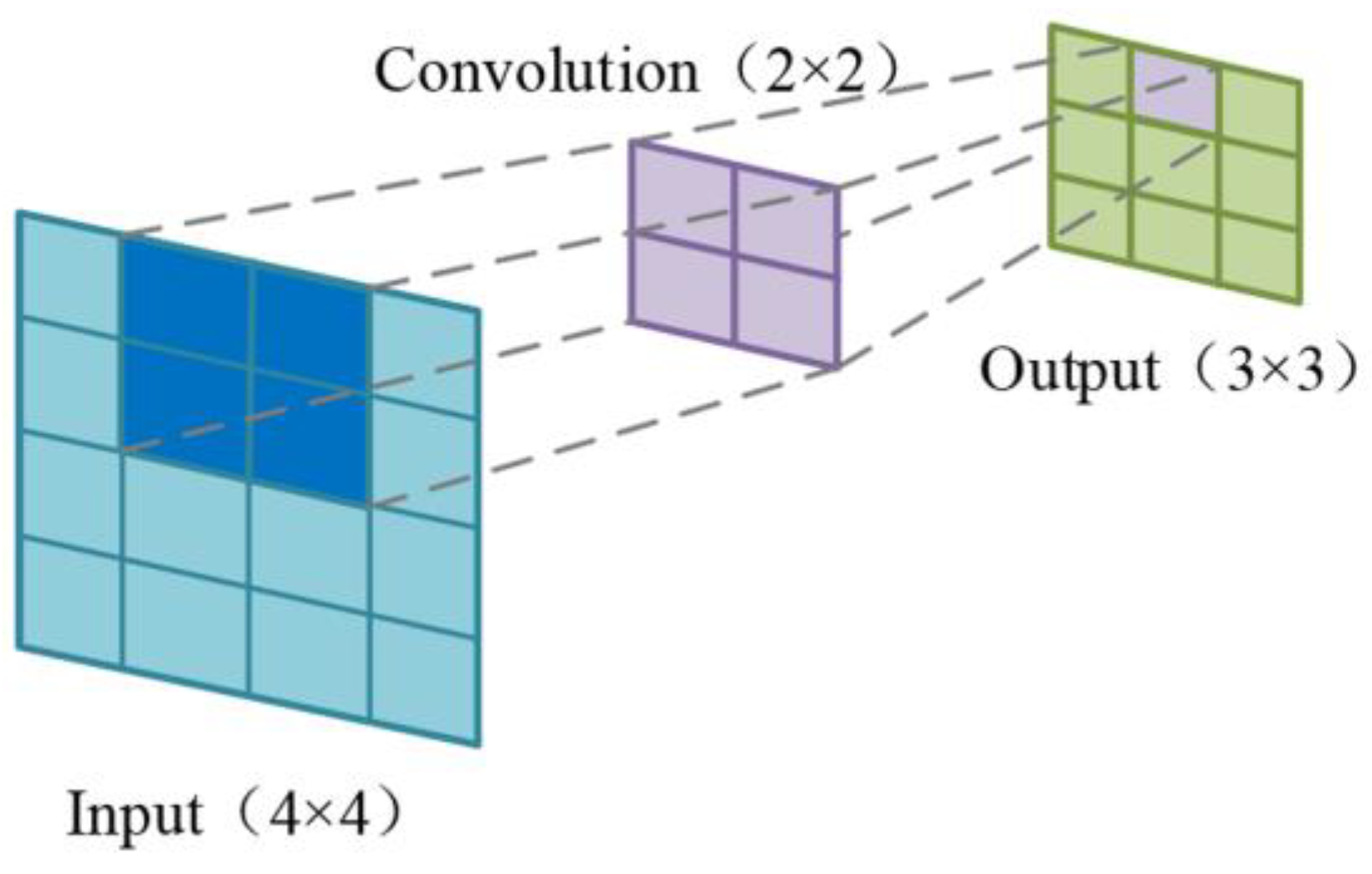
A CNN includes convolutional layers, pooling layers, and fully connected layers. The expression of the convolution operation is as follows.
In Formula (1), is the th feature map output for the th layer, is the number of input feature maps, is the convolution kernel weight matrix of the th layer, is the th feature map of the output of the layer, is the convolution kernel bias matrix of the th layer, and is the activation function.
Figure 1 shows the convolution kernel calculation process. Usually, the pooling layer is added to the convolution layer after reducing the data size to prevent overfitting. The common pooling operations are max pooling and average pooling.
2.2. Deep Residual Network
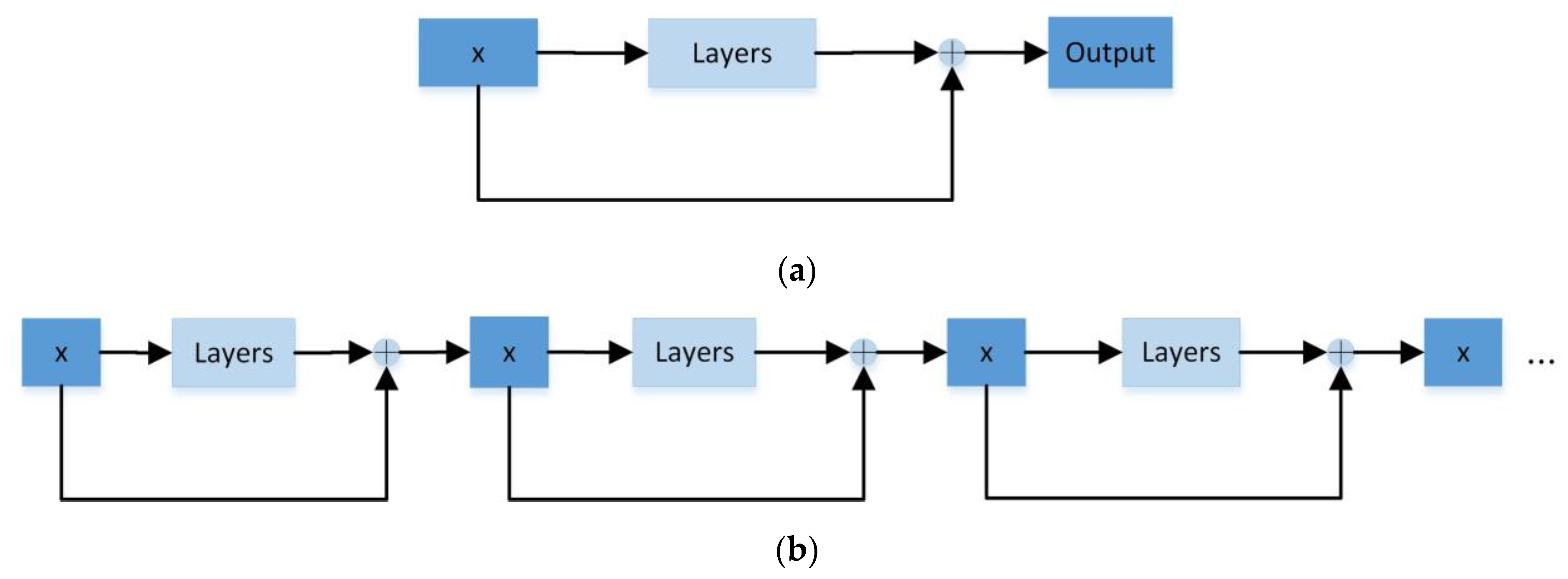
With the development of convolutional neural networks, numerous variants of neural networks have been studied by scholars. A deep residual network (ResNet) [23] was proposed by four scholars from Microsoft Research to solve the problem of gradient disappearance and degradation in deep networks. There are many types of ResNet, such as ResNet18, ResNet34, ResNet50, ResNet101, ResNet152, etc. However, their basic structures are the same—they are made up of multiple layers of identical ResNet blocks stacked repeatedly. The deep residual network achieves jump mapping by adding ResNet blocks, and the inputs and outputs are binary summed to compensate for the lost feature information. In Figure 2, x represents the input to the network, and the layers represent several layers of the network.
2.3. Domain Distribution Difference Measure
There are two very important concepts in transfer learning: domain and task. The domain can be interpreted as a specific domain, and the task is a specific problem that we need to solve. For example, sentiment analysis and entity recognition are two different tasks. In the field of fault diagnosis, transfer tasks are mainly used to solve the problem of unlabeled or less labeled data in the target domain. Fault diagnosis of unlabeled target domain data is performed by network parameters learned using labeled source domain data.
Suppose that the source space , represents the th source domain data and label, and is the total number of samples in the source domain; the target domain space is , where represents the th target domain data; and is the total number of samples of the target domain. The edge distribution of the two domains is allowed to be different, namely . Domain adaptation ensures that the data of different distributions are as close as possible, via certain methods, when the data distribution of the source domain and target domain are different. There are four commonly used methods: (1) methods based on statistical criteria, (2) methods based on structural criteria, (3) methods based on popular criteria, and (4) methods based on graph criteria.
The methods based on statistical criteria use mean or higher-order moments to measure the differences between different domains. Common methods include maximum mean difference (MMD) [24], association alignment distance (CORAL) [25], and joint maximum mean difference (JMMD) [26]. These kinds of methods map the source domain data and the target domain data to the feature space for calculation so that the data distribution difference between the two mapped domains is minimized.
The MMD metric is widely used in domain adaptation. MMD is a kernel learning method that measures the distance between two distributions in a regenerated Hilbert space. The basic idea behind MMD is that if the generating distributions are identical, all the statistics are the same [27]. The distance between the source domain and the target domain is expressed as follows. and are two datasets from the source domain and the target domain, and are the abbreviations for the source domain and target domain, respectively, and are examples of and , and and are the number of samples from the source domain and target domain.
In Formula (2), represents feature mapping and is used to solve the inner product mapped to two high-dimensional vectors. represents the Hilbert space. represents the inner product of the vector.
2.4. Optimal Algorithm
Machine learning algorithms eventually involve parameter optimization problems. Parameter optimization often uses methods based on maximizing posterior probability, minimizing intra-class distance, or constructing a loss function based on network prediction values and actual real values.
In the neural network architecture, the network is often optimized based on the loss function. The appropriate optimization algorithm is used for back propagation to update the network learnable parameters and reduce the loss function value so that the constructed model can output the real label more accurately. Depending on the gradient type, the algorithm can be divided into a gradient optimization algorithm or a gradient-free optimization algorithm. A gradient optimization algorithm is the most commonly used optimization algorithm in deep learning neural networks. Most deep neural networks use stochastic gradient descent (SGD) or its variants for parameter optimization.
3. Multi-Source Subdomain Adaptation Model
3.1. The Structure of the Model
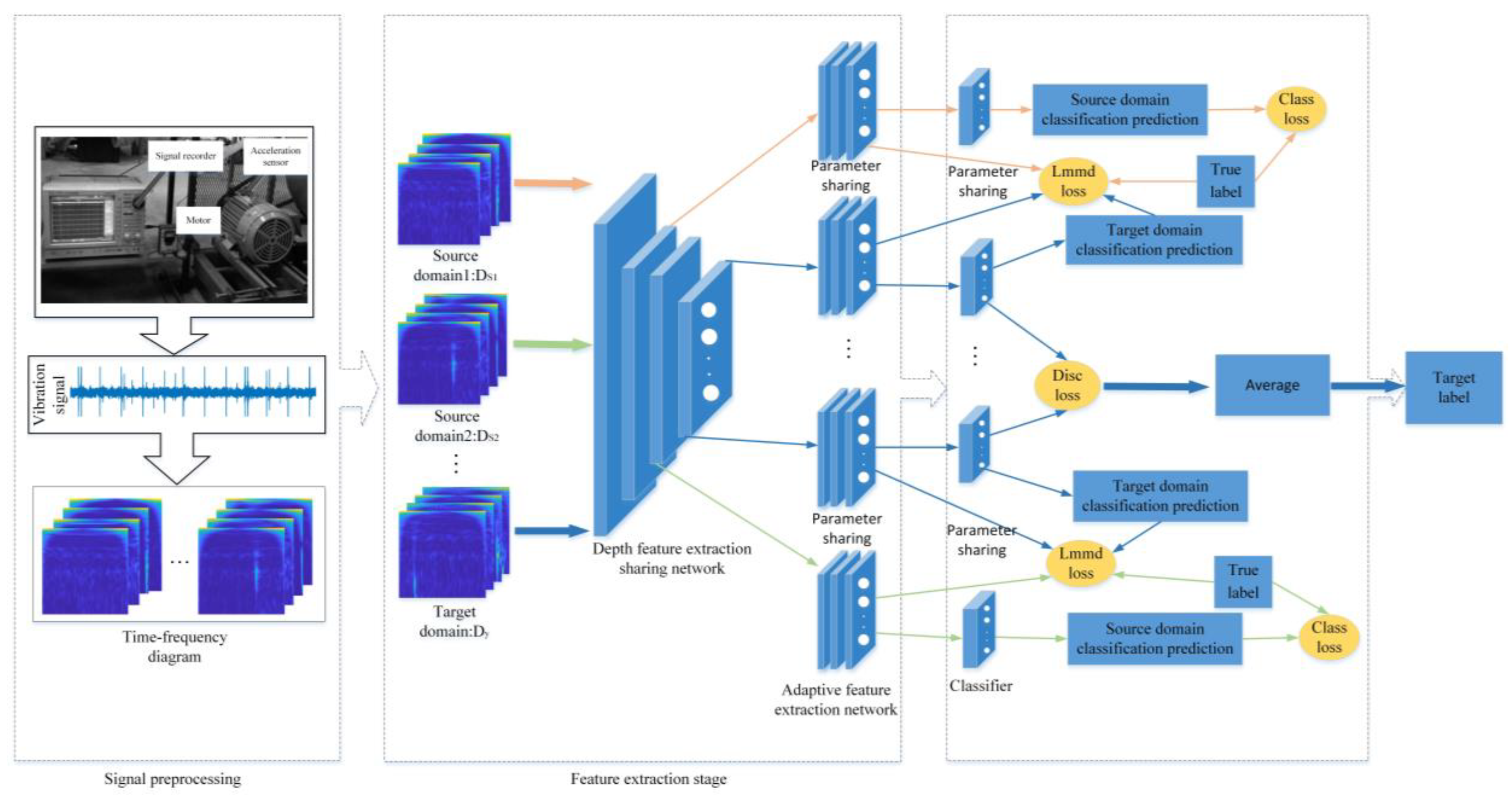
The overall structure of the multi-source subdomain adaptive fault diagnosis model designed in this paper is shown in Figure 3.
It can be seen from Figure 3 that the network mainly includes signal preprocessing, a feature extraction network, network optimization, and state recognition. The specific steps of each stage are as follows.
- (1)
- Signal preprocessing: The bearing vibration signal of Jiangnan University is sampled by an overlapping sampling method to increase the number of samples. Continuous wavelet transform is performed on each type of signal sample using CMOR wavelet to obtain a time–frequency diagram. Meanwhile, source–target data pairs are constructed.
- (2)
- Feature extraction network: The network consists of shared and domain-specific feature extraction networks. First, the data are extracted using a shared feature extraction network. Then, the specific feature extraction network is used to extract the specific features for each group of data.
- (3)
- Network optimization: The total training loss function of the network consists of three parts. In this paper, the local maximum mean difference metric loss function is selected to reduce the distribution difference in each group of data pairs, so that the network can better learn the domain invariant representation. Each group of specific feature extraction networks can extract the domain invariant representation of each pair of source domain and target domain by minimizing losslmmd. N classifiers are trained using labeled source domain data, and the cross-entropy loss between the actual label and the predicted label in the source domain is calculated. Each group of classifiers corresponds to the corresponding lossclass. The loss function lossdisc is used to minimize the error between all classifiers and reduce the classification error near the target domain class boundary. The network training process uses the Ranger optimizer to reduce the total training loss function value.
- (4)
- State recognition: Target domain data are input into the trained network and the diagnostic results are output.
In order to simplify the parameter adjustment process of the network, the model parameters in this paper are basically consistent with those in reference [20]. The literature presents a multi-source domain migration learning method, where the literature not only aligns the distribution of each pair of source and target domains in multiple specific feature spaces, but also aligns the output of the classifier using domain-specific decision boundaries. The literature uses ResNet50 for the shared feature network and employs mmd loss as the domain alignment method. On this basis, the network structure and parameters can be optimized to improve the recognition effect. The model parameters are shown in Table 1.
In Table 1, Conv (,) is the convolution operation, Linear (,) is the fully connected layer, Bn (·) is the batch normalization layer, and ReLU (·) is the activation function layer. represents the number of input neurons, and represents the number of output neurons.
3.2. Continuous Wavelet Transform
The CMOR wavelet is often used in the analysis of seismic data. Owing to the similarity between bearing vibration signals and seismic waves [28], the CMOR wavelet basis can often achieve better results when using bearing fault diagnosis methods.
In continuous wavelet transform, it is assumed that the original signal, , exists. Through the convolution operation between and the wavelet cluster, , the continuous wavelet transform formula is obtained as follows.
In Formulas (3) and (4), and are the expansion factor and displacement factor, respectively, denotes time, and is the wavelet basis function after stretching and displacement.
3.3. Shared Feature Extraction Network
Considering the shallow depth of the neural network and the weak ability to extract features, this paper uses ResNet50 as a shared feature extraction network. ResNet50 contains 50 layers and is divided into 5 stages. The specific parameters of the network are shown in Table 2.
3.4. Local Maximum Mean Discrepancy
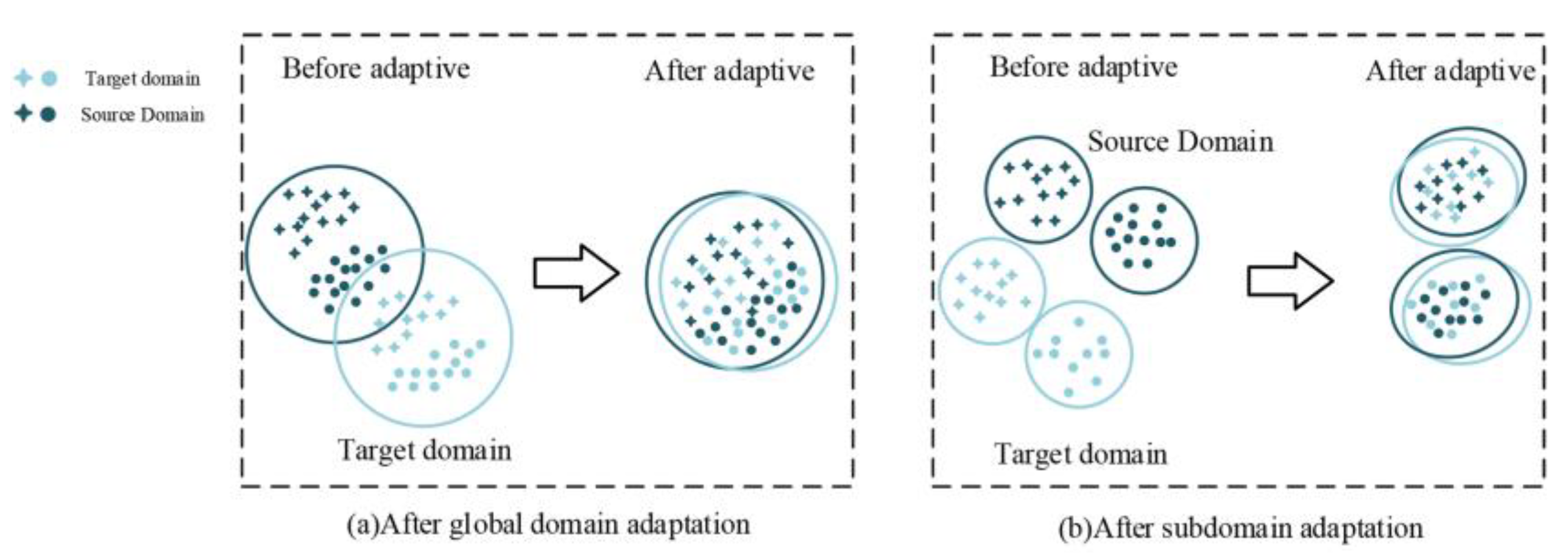
Since MMD mainly learns the global alignment of the source domain and the target domain, it ignores the subdomain relationship between the two domains. After the global domain adaptation alignment, the distribution of the two domains is basically the same, but the data distance of the different subdomains is too close, making the network difficult to classify accurately. Therefore, this paper introduces the local maximum mean difference (LMMD) [27].
In Figure 4, the left side is global domain adaptation and the right side is a subdomain adaptation.
Suppose there are samples in source domain and samples in target domain , where samples and belong to each category, with weights and , and is the th element of the label vector ( is the number of categories). The formulas for LMMD are shown in (5) and (6).
Since cannot be calculated directly, the above equation is transformed. As shown in Formula (7), represents the inner product of the vector.
3.5. Ranger Optimization Algorithm
In order to make the network training more stable and robust, this paper used the Ranger optimization algorithm to optimize the network parameters. The Ranger optimization algorithm uses RAdam [29] and Lookahead [30] as internal and external optimizers, respectively.
The internal optimizer, A, updates the fast weight, , and the update rules of the fast weight are as follows:
where represents the objective function, represents an optimization algorithm, represents sample small batch data, represents the exploration of the th batch, and is the number of iterations.
The update of the slow weight is affected by the fast weight. When the internal optimizer A completes batch explorations, the slow weight update formula is as follows.
3.6. Network Optimization
The calculation formula for classification is as follows.
In Formula (10), represents the classification loss of source domains, is the classifier trained in the source domain of the th group, is a cross-entropy function, is a specific domain feature extraction network, and is a shared feature extraction network.
In the multi-source classifier, the classifier learned by each set of data may have differences in the prediction of target domain samples. Therefore, a loss function that minimizes the differences between different classifiers has been proposed [31], as shown in Formula (11).
There are three optimization objectives in the process of network training:
- Minimize the classification loss function, lossclass, of the source domain dataset;
- Minimize the difference loss, lossdisc, between different classifiers;
- Minimize the domain invariant, losslmmd, of the source and target domain datasets.
Then, the expression of is as follows:
where is the equilibrium hyperparameter.
4. Experiments and Analysis
4.1. Experimental Data
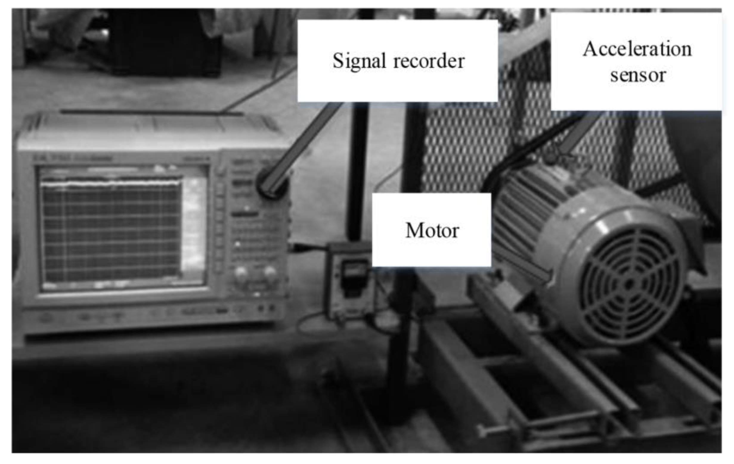
The open dataset of the China Jiangnan University (JNU) bearing fault dataset [32] was selected to verify the validity of the model. The experimental platform is shown in Figure 5. The platform consists of an inductor motor (Mitsubishi SB-JR), accelerometer (PCB MA352A60), and signal conditioner (PCB ICP Model 480C02).
There are four states in the collected bearing data: normal, inner ring fault, outer ring fault, and rolling element fault. The experiment was conducted at 600 r/min, 800 r/min, and 1000 r/min, and different speeds were taken to represent different tasks: dataset A represents the data collected at 600 r/min, B represents the data collected at 800 r/min, and C represents the data collected at 1000 r/min. Datasets A, B, and C are composed of four health states [33]. The health status and corresponding labels are shown in Table 3.
The number of points in each state is 410,112, and 1024 points are intercepted as a group of samples by overlapping sampling, and 800 groups of samples for each state are obtained. The final A, B, and C data sets have 3200 samples. Before the experiment, CMOR wavelet was used to perform wavelet transform on all samples to obtain time–frequency image samples.
The code uses Pytorch as the deep learning framework [34] and a Windows 10 operating system. The experiments were set to a number of 32 samples per batch, the initial learning rate was set to 0.0001, and the total number of training rounds was set to 1500. All compared methods, except the method proposed in this paper, use SGD [35] to optimize the network model.
4.2. Comparative Analysis of the Results of Different Domain Adaptation Methods
In order to verify the effectiveness of the distribution difference measurement method in this paper, it was first compared with several common adaptive methods. In the performance of migration experiments for the different adaptive methods, when the B and C datasets are selected as the source domains and A is selected as the target domain, the task is represented by B-C→A; when datasets A and C are selected as the source domains and B is selected as the target domain, the task is represented by A-C→B. A-B→C represents the task when the A and B datasets are selected as the source domains and C is selected as the target domain.
4.2.1. Visual Comparative Analysis of Output Features
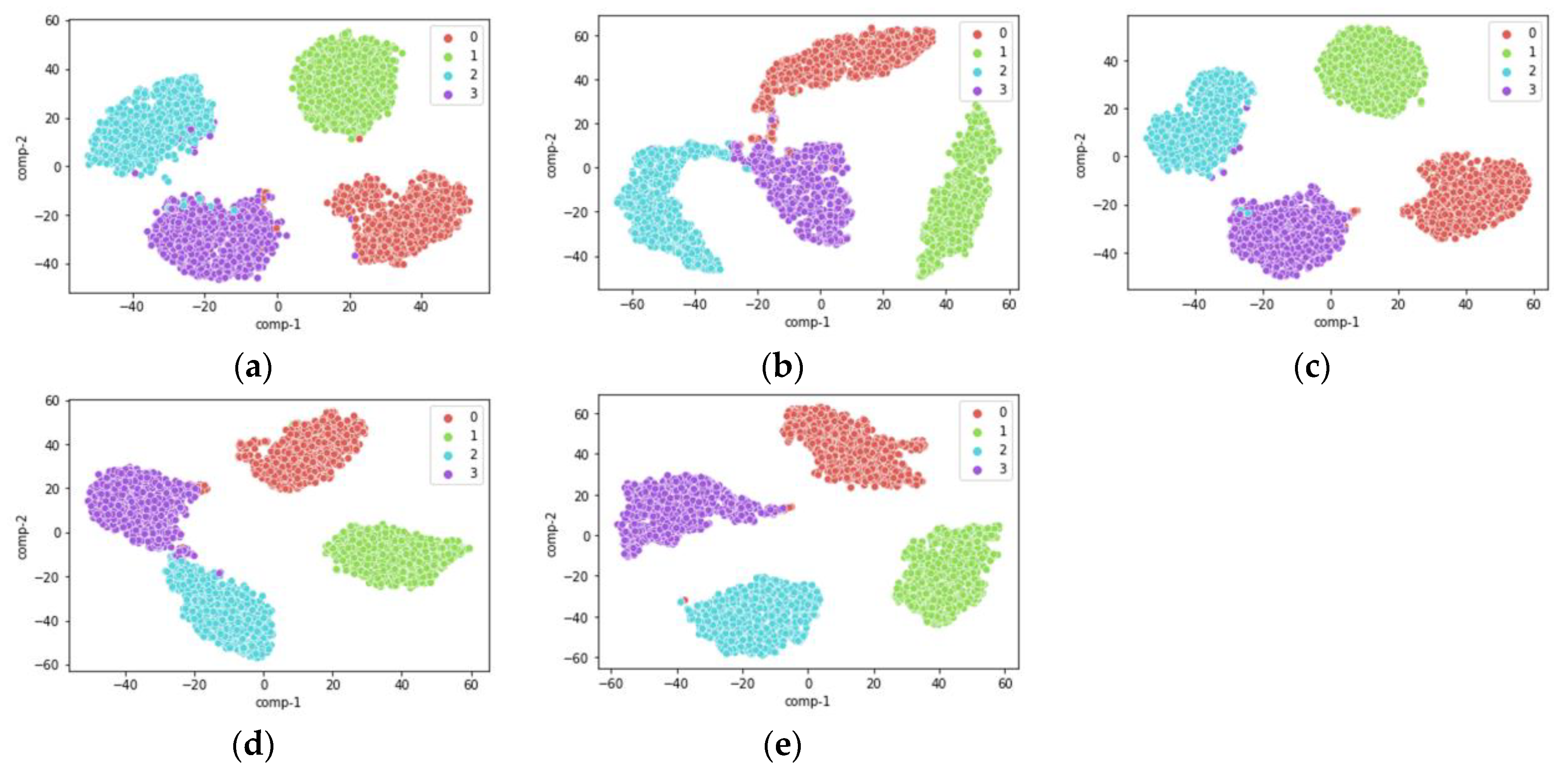
In order to intuitively demonstrate the effectiveness of the proposed method, t-distribution stochastic neighbor embedding (t-SNE [36]) was introduced for the multi-source migration task A-C→B. T-SNE is a nonlinear dimensionality reduction algorithm. Because it can clearly show the relationship between different categories and clusters, it is often used for visualization in the field of fault diagnosis.
The target domain samples are input into the trained network, and the fault features extracted from the last layer of the network are reduced to a two-dimensional plane. The results are shown in Figure 6, where different colors represent different class labels. It can be seen that there is still more cross-over after extracting features using the four comparison methods (a–d). After feature extraction using the proposed method, the four classes of faulty samples have basically been separated, and the target samples can be better classified. The specific recognition accuracy is shown in Table 4. It can be observed that the recognition accuracy of method (a) is 97.81%, the recognition accuracy of method (b) is 98.53%, the recognition accuracy of method (c) is 98.75%, the recognition accuracy of method (d) is 98.81%, and the recognition accuracy of method (e) is 99.65%, which is higher than the other four methods.
4.2.2. Comparative Analysis of Diagnostic Results
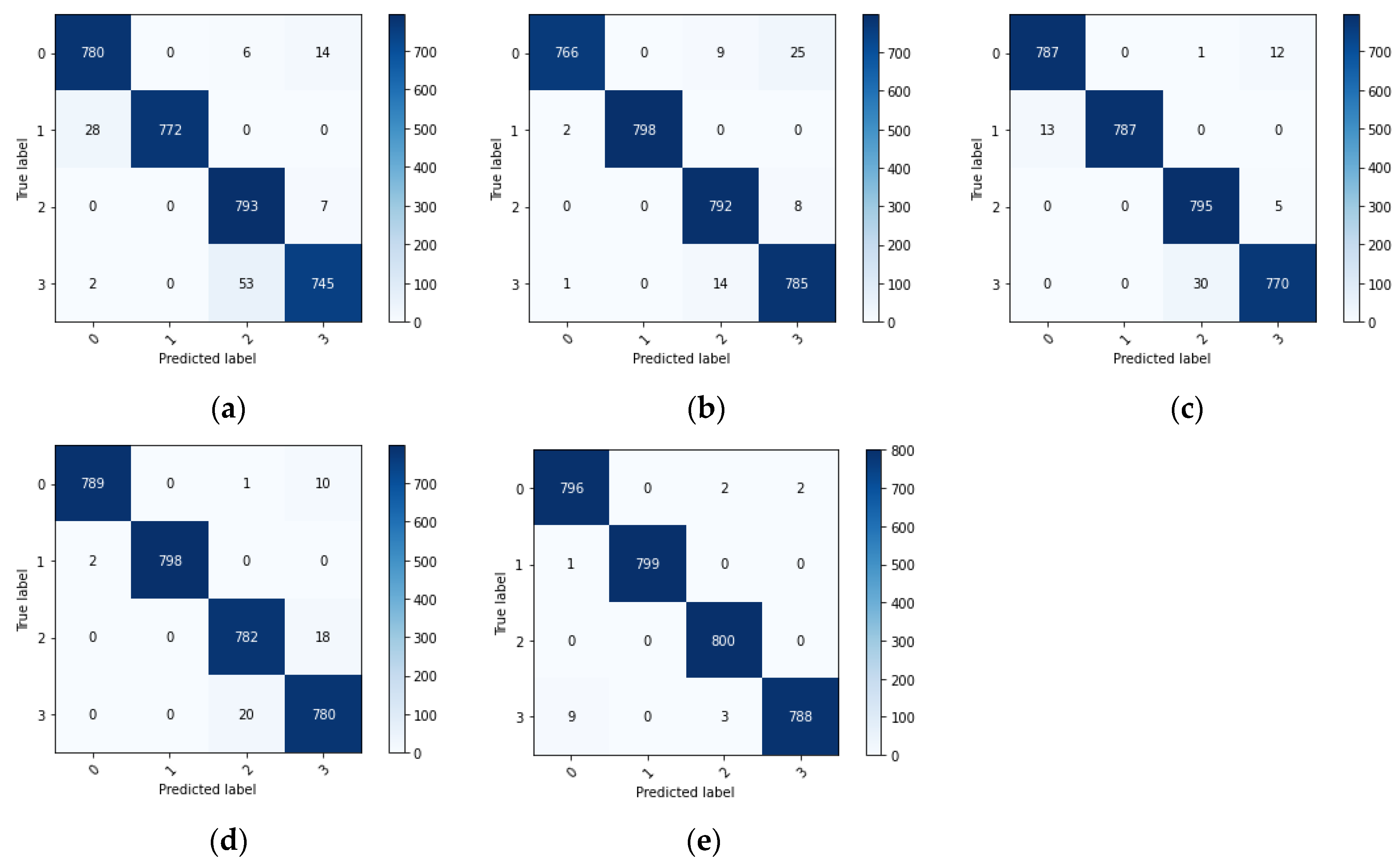
Figure 7 illustrates the confusion matrix of the output categories after performing fault diagnosis for tasks A-C→B. The horizontal coordinates represent the predicted categories of the target domain samples and the vertical coordinates represent the true labels of the target domain samples. From the confusion matrix, it can be seen that if the four methods (a–d) are utilized for fault diagnosis, there are 110, 59, 71, and 51 target domain samples that have been misclassified, respectively. However, after using the proposed method, there are only 17 sample classification errors in 3200 target domain samples. Nine rolling element fault samples were identified as normal state, three rolling element fault samples were identified as outer ring faults, one inner ring fault sample was identified as normal, two normal state samples were identified as outer ring faults, two normal state samples were identified as rolling element faults, and the remaining target domain samples were all correctly classified. The overall diagnostic accuracy was 99.47%.
4.2.3. Comparative Analysis of Diagnostic Accuracy and Change Curve
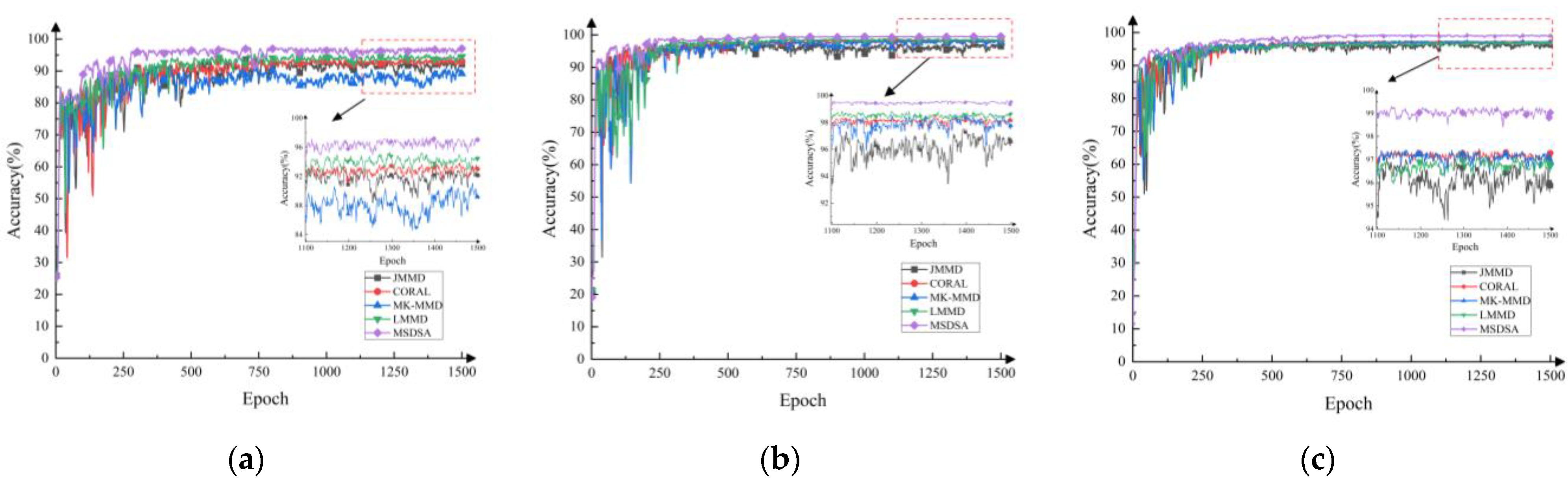
The diagnostic accuracies of the different adaptive methods for three sets of migration tasks are shown in Table 4. Figure 8 shows the variation curve for target domain sample accuracy with the number of iterations in the three sets of tasks. In order to show the contrast effect more clearly, the change curve of the number of iterations greater than 1100 times is locally amplified.
In Figure 8, the change curves, presented in different colors, represent different adaptive methods. It can be seen that, compared with the other four methods, the proposed method has smaller random fluctuations in the three groups of tasks and that the training effect is more stable. More specific information can be seen in Table 4. The proposed method achieves the highest diagnostic accuracy in all three tasks. The diagnostic accuracies of the proposed method in task A-C→B, task A-B→C, and task B-C→A were 99.65%, 99.34%, and 97.40%, respectively. Compared with the other four methods, the diagnostic accuracy is improved by 2.03–8.06%, 0.84–1.84%, and 1.84–2.31%, respectively. This shows that, compared with global domain adaptation, the improvement in the sub-domain adaptation can learn the fine-grained information of each category and can align the distribution of the sub-domains of the same category more effectively. Compared with the LMMD method, the diagnostic accuracy of the proposed method is improved by 2.03%, 0.84%, and 1.97%, respectively. It can be shown that the Ranger optimizer can train the network parameters more effectively and achieve better training results.
4.3. Comparative Analysis of Single-Source Domain and Multi-Source Domain Transfer Learning Task Results
In order to verify the performance of the proposed method more objectively [37], single-source domain and multi-source domain learning were performed on three groups of transfer learning tasks. The model structure and parameters remained unchanged. The experimental results are shown in Table 5.
4.3.1. Visual Comparative Analysis of Output Features
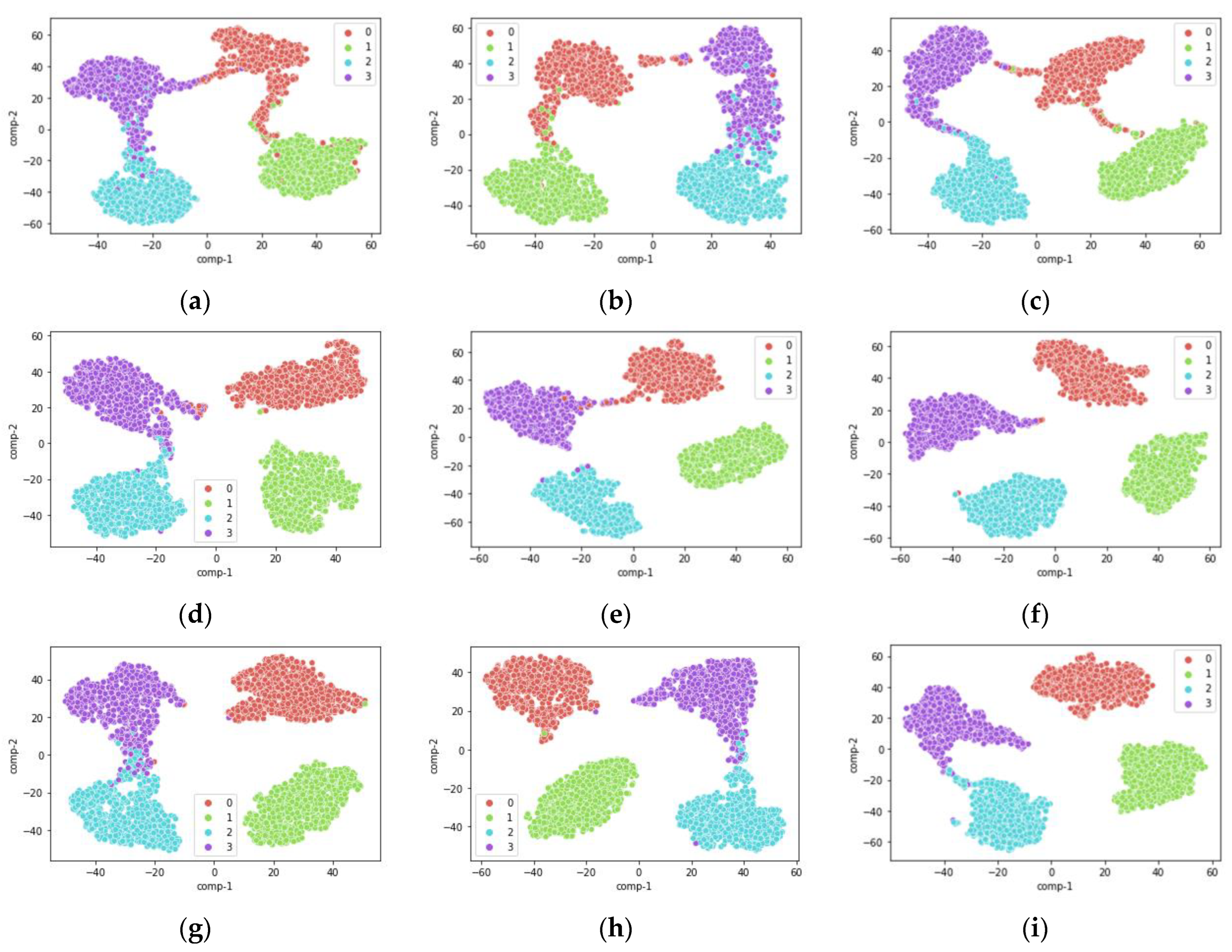
Figure 9 shows the fault feature visualizations of the output from the target domain samples by the last layer of the fault diagnosis network. Like the previous comparison method, the fault feature is reduced to a two-dimensional plane. In the three images in each row, the target domain of the transfer learning task is the same.
From Figure 9, we can see that the single-source domain transfer learning tasks (a), (b), (d), (e), (g), and (h) all have more overlap problems, and the fault diagnosis network has difficulty in classifying them accurately. In contrast, there is less overlap between categories in the multi-source domain migration learning tasks (c), (f), and (i).
4.3.2. Comparative Analysis of Diagnostic Results
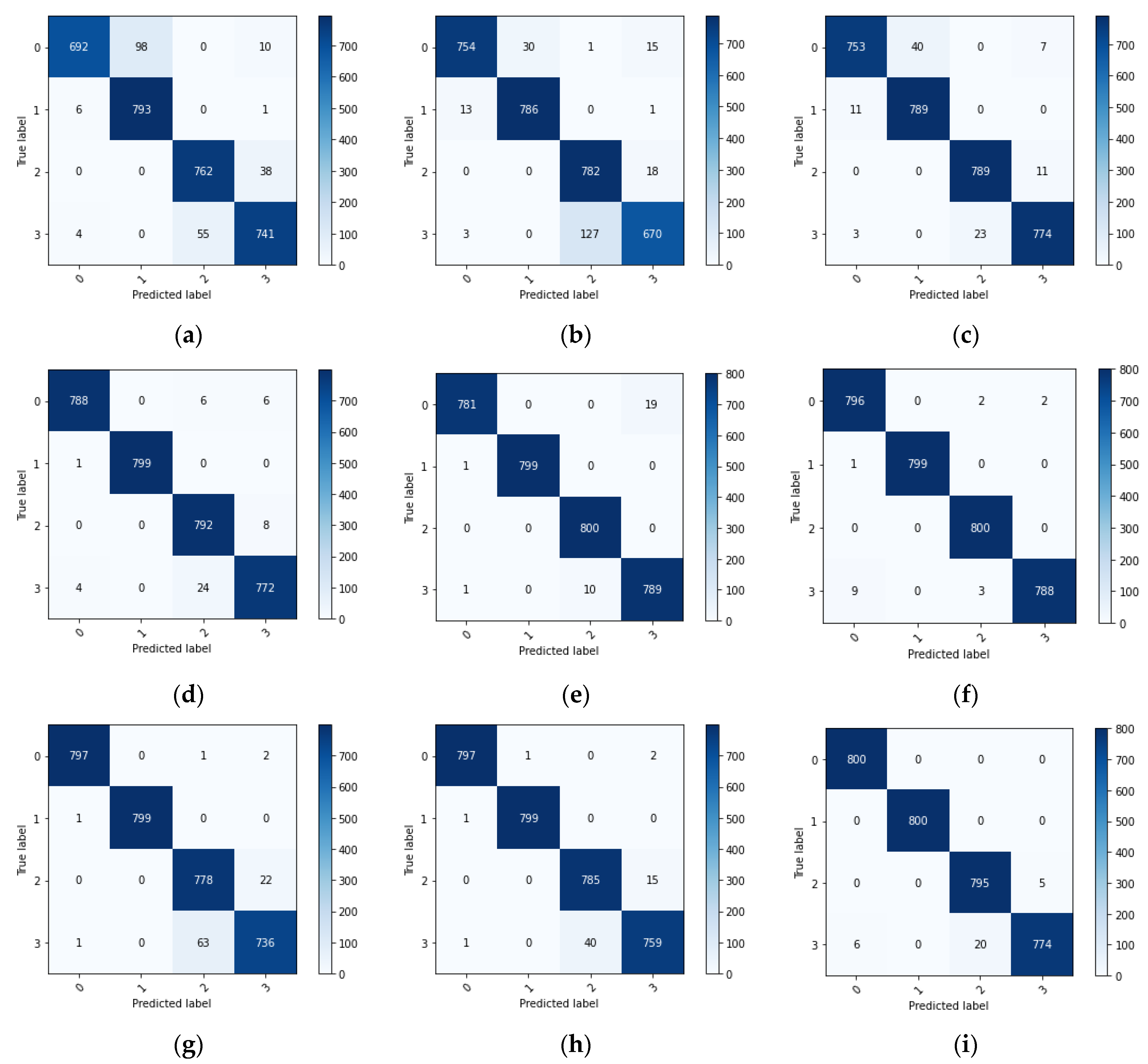
Figure 10 shows the confusion matrix of the diagnostic results of the single-source domain and multi-source domain migration learning tasks. The images are arranged in the same order as in Figure 9. It can be seen from Figure 10 that the multi-source domain tasks (c), (f), and (i) can reduce the classification errors for the target domain samples compared to the single-source domain tasks (a), (b), (d), (e), (g), and (h).
4.3.3. Comparative Analysis of Diagnostic Accuracy and Change Curve
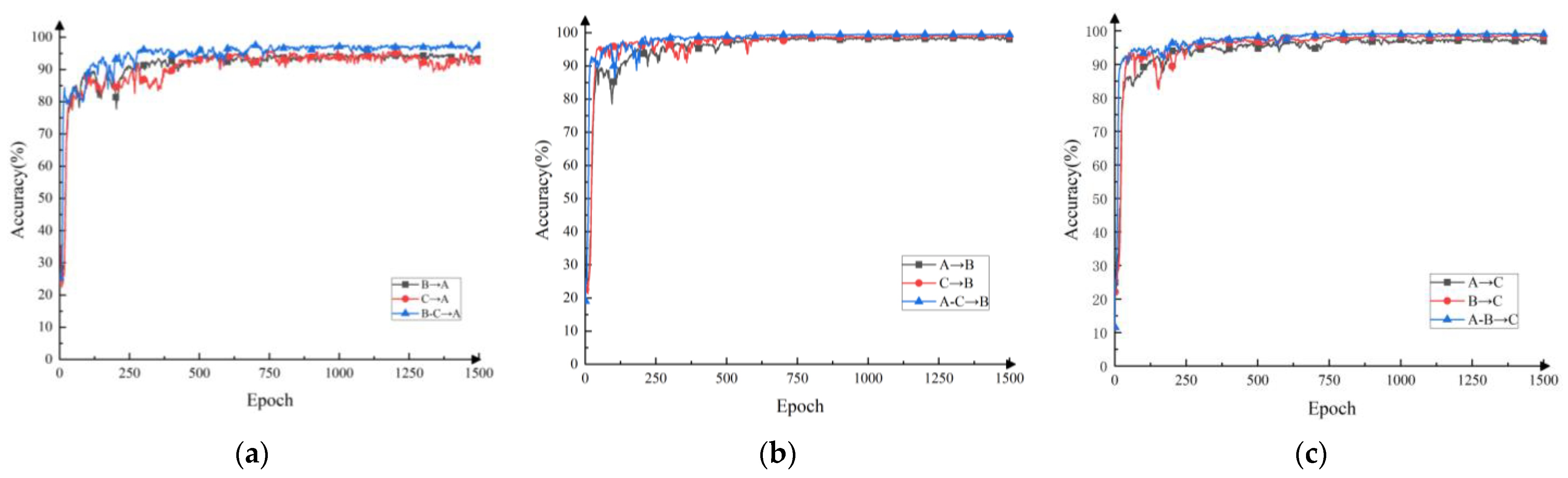
Figure 11 shows the change curves of three different target domains on single-source domain and multi-source domain transfer learning tasks. The gray and red curves in the figure represent the single-source domain tasks. The blue curve represents the multi-source domain task. The final fault diagnosis accuracy results are shown in Table 5.
It can be seen from Figure 11 and Table 5 that the accuracy of the multi-source domain fault diagnosis method is significantly higher than the corresponding single-source domain fault diagnosis method, which can better classify the target domain samples. For example, the accuracy of the multi-source domain method, B-C→A, can reach 97.78%, whereas the diagnostic accuracy of the single-source domain methods, B→A and C→A, can only reach 95.09% and 96.13%, and the classification accuracy is improved by 1.97% and 1.56%, respectively. To a certain extent, this can be explained that under complex working conditions, a multi-source domain can learn richer domain-invariant feature information more effectively than a single-source domain.
5. Discussion
In traditional research on transfer learning methods, only single-source unsupervised adaptation is often considered. Whereas, in practical scenarios, multiple sets of source domain data can be obtained, and the distribution of different source domain data may be different. Therefore, on the above basis, multi-source unsupervised adaptation has been widely concerned. A key assumption of multi-source transfer work is that multiple source domains contain complementary diagnostic knowledge [38] so that the combined knowledge can be used for diagnostic tasks in the target domain.
The optimization function of MSDSD proposed in this paper consists of three parts: the cross entropy loss of the source domain, the local maximum mean error function for measuring the distribution difference between domains, and the loss function for minimizing the difference between all classifiers. Through network iteration, a more stable fault diagnosis network of variable condition bearings is finally trained. On the other hand, considering that the variable condition fault diagnosis network may have unstable training, this paper combines the Ranger optimizer to improve the stability of network training.
The model structure and parameters in this paper were mostly set based on the research results of related papers. The model parameters could have influenced either the diagnosis process or results to a varying extent. Therefore, the model structure and parameters ought to be investigated further. Different adaptive methods can determine the transferable features learned on the source domain, so follow-up work can be carried out from this aspect.
6. Conclusions
With the aim of solving the problem of insufficient feature information extracted using a single-source transfer learning method, this paper proposed a multi-source sub-domain adaptive deep transfer learning fault diagnosis method that uses the LMMD as the adaptive method and a Ranger optimizer to optimize the network parameters. Finally, the method was evaluated using the JNU bearing dataset of Jiangnan University. The conclusions obtained are as follows:
- (1)
- The subdomain adaptive method can better align the distribution difference between the source domain and the target domain;
- (2)
- Using multi-source domain learning can extract richer information;
- (3)
- Using the Ranger optimizer instead of a mainstream optimizer can further improve the accuracy of network training.
Compared to the different domain adaptation methods and a single-source domain experiment task, the effectiveness of the proposed method was proven.
Author Contributions
Conceptualization, F.X., S.X. and L.W.; methodology, F.X. and L.W.; validation, L.W.; formal analysis, F.X. and L.W.; investigation, L.W.; resources, F.X.; writing—original draft preparation, L.W.; writing—review and editing, F.X. and L.W.; visualization, L.W.; supervision, F.X. and S.X.; project administration, F.X. and S.X.; funding acquisition, F.X., H.Z. and S.X. All authors have read and agreed to the published version of the manuscript.
Funding
This research was supported by the National Natural Science Foundation of China (52265068), the Natural Science Foundation of Jiangxi Province (20224BAB204050), Carrier and Equipment Key Laboratory Project of the Ministry of Education (KLCEZ2022-02), and the Project of the Jiangxi Provincial Department of Education (GJJ2200627).
Institutional Review Board Statement
Not applicable.
Informed Consent Statement
Not applicable.
Data Availability Statement
The data that support the findings of this study are openly available in http://www.52phm.cn/blog/detail/52 (accessed on 1 April 2023) and https://pan.baidu.com/s/1uRj_MGeS7UdLhPZKurIR6g (accessed on 1 April 2022).
Conflicts of Interest
The authors declare no conflict of interest.
References
- Xiao, Q.; Li, S.; Zhou, L.; Shi, W. Improved variational mode decomposition and CNN for intelligent rotating machinery fault diagnosis. Entropy 2022, 24, 908. [Google Scholar] [CrossRef] [PubMed]
- Han, T.; Li, Y.-F.; Qian, M. A hybrid generalization network for intelligent fault diagnosis of rotating machinery under unseen working conditions. IEEE Trans. Instrum. Meas. 2021, 70, 1–11. [Google Scholar] [CrossRef]
- Zhang, W.; Li, C.; Peng, G.; Chen, Y.; Zhang, Z. A deep convolutional neural network with new training methods for bearing fault diagnosis under noisy environment and different working load. Mech. Syst. Signal Process. 2018, 100, 439–453. [Google Scholar] [CrossRef]
- Jin, J.; Xu, Z.; Li, C.; Zhou, L.; Miao, W. Research on fault diagnosis of rolling bearings based on deep learning and support vector machine. Therm. Power Eng. 2022, 37, 176–184. [Google Scholar] [CrossRef]
- Yang, S.; Kong, X.; Wang, Q.; Li, Z.; Cheng, H.; Yu, L. A multi-source ensemble domain adaptation method for rotary machine fault diagnosis. Measurement 2021, 186, 110213. [Google Scholar] [CrossRef]
- Junbo, T.; Weining, L.; Juneng, A.; Xueqian, W. Fault diagnosis method study in roller bearing based on wavelet transform and stacked auto-encoder. In Proceedings of the 27th Chinese control and decision conference (2015 CCDC), Qingdao, China, 23–25 May 2015; pp. 4608–4613. [Google Scholar]
- Shao, S.; McAleer, S.; Yan, R.; Baldi, P. Highly accurate machine fault diagnosis using deep transfer learning. IEEE Trans. Ind. Inform. 2018, 15, 2446–2455. [Google Scholar] [CrossRef]
- Yan, R.; Shen, F.; Sun, C.; Chen, X. Knowledge transfer for rotary machine fault diagnosis. IEEE Sens. J. 2019, 20, 8374–8393. [Google Scholar] [CrossRef]
- Pan, S.J.; Tsang, I.W.; Kwok, J.T.; Yang, Q. Domain adaptation via transfer component analysis. IEEE Trans. Neural Netw. 2010, 22, 199–210. [Google Scholar] [CrossRef] [Green Version]
- Long, M.; Wang, J.; Ding, G.; Sun, J.; Yu, P.S. Transfer feature learning with joint distribution adaptation. In Proceedings of the IEEE International Conference on Computer Vision, Sydney, Australia, 1–8 December 2013; pp. 2200–2207. [Google Scholar]
- Wang, J.; Chen, Y.; Hao, S.; Feng, W.; Shen, Z. Balanced distribution adaptation for transfer learning. In Proceedings of the 2017 IEEE International Conference on Data Mining (ICDM), New Orleans, LA, USA, 18–21 November 2017; pp. 1129–1134. [Google Scholar]
- Zhu, J.; Chen, N.; Shen, C. A new deep transfer learning method for bearing fault diagnosis under different working conditions. IEEE Sens. J. 2019, 20, 8394–8402. [Google Scholar] [CrossRef]
- Qian, W.; Li, S.; Yi, P.; Zhang, K. A novel transfer learning method for robust fault diagnosis of rotating machines under variable working conditions. Measurement 2019, 138, 514–525. [Google Scholar] [CrossRef]
- Cheng, C.; Zhou, B.; Ma, G.; Wu, D.; Yuan, Y. Wasserstein distance based deep adversarial transfer learning for intelligent fault diagnosis with unlabeled or insufficient labeled data. Neurocomputing 2020, 409, 35–45. [Google Scholar] [CrossRef]
- Yang, B.; Lei, Y.; Jia, F.; Xing, S. An intelligent fault diagnosis approach based on transfer learning from laboratory bearings to locomotive bearings. Mech. Syst. Signal Process. 2019, 122, 692–706. [Google Scholar] [CrossRef]
- Wang, X.; He, H.; Li, L. A hierarchical deep domain adaptation approach for fault diagnosis of power plant thermal system. IEEE Trans. Ind. Inform. 2019, 15, 5139–5148. [Google Scholar] [CrossRef]
- Duan, L.; Xu, D.; Tsang, I.W.-H. Domain adaptation from multiple sources: A domain-dependent regularization approach. IEEE Trans. Neural Netw. Learn. Syst. 2012, 23, 504–518. [Google Scholar] [CrossRef]
- Liu, H.; Shao, M.; Fu, Y. Structure-preserved multi-source domain adaptation. In Proceedings of the 2016 IEEE 16th International Conference on Data Mining (ICDM), Barcelona, Spain, 12–15 December 2016; pp. 1059–1064. [Google Scholar]
- Mansour, Y.; Mohri, M.; Rostamizadeh, A. Domain adaptation with multiple sources. Adv. Neural Inf. Process. Syst. 2008, 21, 1041–1048. [Google Scholar]
- Zhu, Y.; Zhuang, F.; Wang, D. Aligning domain-specific distribution and classifier for cross-domain classification from multiple sources. In Proceedings of the AAAI Conference on Artificial Intelligence, Honolulu, HI, USA, 29–31 January 2019; pp. 5989–5996. [Google Scholar]
- Rezaeianjouybari, B.; Yi, S. A Novel Deep Multi-Source Domain Adaptation Framework for Bearing Fault Diagnosis Based on Feature-level and Task-specific Distribution Alignment. Measurement 2021, 178, 109359. [Google Scholar] [CrossRef]
- Zhan, K. A CNN-LSTM ship motion extreme value prediction model. Shanghai Jiaotong Univ. 2022, 1–9. [Google Scholar] [CrossRef]
- He, K.; Zhang, X.; Ren, S.; Sun, J. Deep residual learning for image recognition. In Proceedings of the IEEE Conference on Computer Vision and Pattern Recognition, Las Vegas, NV, USA, 27–30 June 2016; pp. 770–778. [Google Scholar]
- Tzeng, E.; Hoffman, J.; Zhang, N.; Saenko, K.; Darrell, T. Deep domain confusion: Maximizing for domain invariance. arXiv 2014, arXiv:1412.3474. [Google Scholar]
- Sun, B.; Feng, J.; Saenko, K. Return of frustratingly easy domain adaptation. In Proceedings of the AAAI Conference on Artificial Intelligence, Phoenix, AZ, USA, 12–17 February 2016. [Google Scholar]
- Long, M.; Zhu, H.; Wang, J.; Jordan, M.I. Deep transfer learning with joint adaptation networks. In Proceedings of the International Conference on Machine Learning, Sydney, Australia, 6–11 August 2017; pp. 2208–2217. [Google Scholar]
- Zhu, Y.; Zhuang, F.; Wang, J.; Ke, G.; Chen, J.; Bian, J.; Xiong, H.; He, Q. Deep subdomain adaptation network for image classification. IEEE Trans. Neural Netw. Learn. Syst. 2020, 32, 1713–1722. [Google Scholar] [CrossRef] [PubMed]
- Song, L. Research on Fault Diagnosis Methods Based on Attention Mechanism and Deep Learning. Master’s Thesis, Southwest University of Science and Technology, Mianyang, China, 2021. [Google Scholar]
- Liu, L.; Jiang, H.; He, P.; Chen, W.; Liu, X.; Gao, J.; Han, J. On the variance of the adaptive learning rate and beyond. arXiv 2019, arXiv:1908.03265. [Google Scholar]
- Zhang, M.; Lucas, J.; Ba, J.; Hinton, G.E. Lookahead optimizer: K steps forward, 1 step back. In Proceedings of the Advances in Neural Information Processing Systems, Vancouver, BC, Canada, 8–14 December 2019; pp. 9597–9608. [Google Scholar]
- Xu, R.; Chen, Z.; Zuo, W.; Yan, J.; Lin, L. Deep cocktail network: Multi-source unsupervised domain adaptation with category shift. In Proceedings of the IEEE Conference on Computer Vision and Pattern Recognition, Salt Lake City, UT, USA, 18–23 June 2018; pp. 3964–3973. [Google Scholar]
- Li, K. Available online: http://www.52phm.cn/blog/detail/52 (accessed on 2 February 2023).
- Sun, B.; Saenko, K. Deep coral: Correlation alignment for deep domain adaptation. In Proceedings of the Computer Vision–ECCV 2016 Workshops, Amsterdam, The Netherlands, 8–10, 15–16 October 2016; pp. 443–450. [Google Scholar]
- Braun, S. LSTM benchmarks for deep learning frameworks. arXiv 2018, arXiv:1806.01818. [Google Scholar]
- Robbins, H.; Monro, S. A stochastic approximation method. Ann. Math. Stat. 1951, 22, 400–407. [Google Scholar] [CrossRef]
- Van der Maaten, L.; Hinton, G. Visualizing data using t-SNE. J. Mach. Learn. Res. 2008, 9, 2579–2605. [Google Scholar]
- Kim, B.; Kim, D.H.; Park, S.H.; Kim, J.; Lee, J.-G.; Ye, J.C. CycleMorph: Cycle consistent unsupervised deformable image registration. Med. Image Anal. 2021, 71, 102036. [Google Scholar] [CrossRef]
- Yang, B.; Xu, S.; Lei, Y.; Lee, C.-G.; Stewart, E.; Roberts, C. Multi-source transfer learning network to complement knowledge for intelligent diagnosis of machines with unseen faults. Mech. Syst. Signal Process. 2022, 162, 108095. [Google Scholar] [CrossRef]
Figure 1.
Convolution kernel calculation process.

Figure 2.
(a) Residual block structure. (b) Repeated residual block structure.

Figure 3.
Multi-source sub-domain fault diagnosis network structure.

Figure 4.
Domain adaptation.

Figure 5.
JNU bearing test bench.

Figure 6.
Feature visualization: (a) JMMD; (b) CORAL; (c) MK-MMD; (d) LMMD; (e) MSDSA.

Figure 7.
Confusion matrix: (a) JMMD; (b) CORAL; (c) MK-MMD; (d) LMMD; (e) MSDSA.

Figure 8.
Comparison of different adaptive methods in three groups of tasks: (a) B-C→A; (b) A-C→B; (c) A-B→C.
Figure 8.
Comparison of different adaptive methods in three groups of tasks: (a) B-C→A; (b) A-C→B; (c) A-B→C.

Figure 9.
Feature visualization: (a) B→A; (b) C→A; (c) B-C→A; (d) A→B; (e) C→B; (f) A-C→B; (g) A→C; (h) B→C; (i) A-B→C.
Figure 9.
Feature visualization: (a) B→A; (b) C→A; (c) B-C→A; (d) A→B; (e) C→B; (f) A-C→B; (g) A→C; (h) B→C; (i) A-B→C.

Figure 10.
Confusion matrix: (a) B→A; (b) C→A; (c) B-C→A; (d) A→B; (e) C→B; (f) A-C→B; (g) A→C; (h) B→C; (i) A-B→C.
Figure 10.
Confusion matrix: (a) B→A; (b) C→A; (c) B-C→A; (d) A→B; (e) C→B; (f) A-C→B; (g) A→C; (h) B→C; (i) A-B→C.

Figure 11.
Comparison of single-source domain and multi-source domain transfer learning tasks in different target domains: (a) the target domain is dataset A; (b) the target domain is dataset B; (c) the target domain is dataset C.
Figure 11.
Comparison of single-source domain and multi-source domain transfer learning tasks in different target domains: (a) the target domain is dataset A; (b) the target domain is dataset B; (c) the target domain is dataset C.


Table 1.
The overall structure and parameters of the network.
| Network Structure | Network Parameter |
|---|---|
| Feature extraction network | ResNet50(share)- Conv (2048,256)-Bn()- Conv (256,256)-Bn()-Conv(256,256)-Bn()-ReLU() |
| Classifier | Linear(256,4) |
Table 2.
ResNet50 network structure.
| Network Structure | Type | Receptive Field Size |
|---|---|---|
| Input | 224 × 224 × 3 | |
| Con1 | Convolution layer | |
| Max pool | Maximum pooling layer | |
| Conv2_x | Residual block 1 × 3 | |
| Conv3_x | Residual block 1 × 4 | |
| Conv4_x | Residual block 1 × 6 | |
| Conv5_x | Residual block 1 × 3 | |
| Average | Average pooling layer |
Table 3.
JNU bearing dataset settings.
| Dataset | State of Health | Rotating Speed(R/Min) | Label | Sample Size |
|---|---|---|---|---|
| A | Normal | 600 | 0 | 800 |
| A | Inner ring fault | 600 | 1 | 800 |
| A | Outer ring fault | 600 | 2 | 800 |
| A | Rolling element fault | 600 | 3 | 800 |
| B | Normal | 800 | 0 | 800 |
| B | Inner ring fault | 800 | 1 | 800 |
| B | Outer ring fault | 800 | 2 | 800 |
| B | Rolling element fault | 800 | 3 | 800 |
| C | Normal | 1000 | 0 | 800 |
| C | Inner ring fault | 1000 | 1 | 800 |
| C | Outer ring fault | 1000 | 2 | 800 |
| C | Rolling element fault | 1000 | 3 | 800 |
Table 4.
Multi-source domain fault classification accuracy of different adaptive methods.
| Adaptive Method | JMMD | CORAL | MK-MMD | LMMD | MSDSA | Increase Percentage (%) | |
|---|---|---|---|---|---|---|---|
| Test | |||||||
| B-C→A | 93.87% | 94.00% | 89.34% | 95.37% | 97.40% | 2.03–8.06% | |
| A-C→B | 97.81% | 98.53% | 98.75% | 98.81% | 99.65% | 0.84–1.84% | |
| A-B→C | 97.03% | 97.47% | 97.50% | 97.37% | 99.34% | 1.84–2.31% | |
| Average | 96.24% | 96.67% | 95.20% | 97.18% | 98.80% | 1.62–3.6% | |
Table 5.
Comparison of fault diagnosis results between single-source domain and multi-source domain migration.
Table 5.
Comparison of fault diagnosis results between single-source domain and multi-source domain migration.
| Task | Accuracy | Task | Accuracy | Increase Percentage (%) |
|---|---|---|---|---|
| B-C→A | 97.78% | B→A C→A | 95.09% 96.13% | 2.69% 1.65% |
| A-C→B | 99.65% | A→B C→B | 98.72% 99.28% | 0.93% 0.37% |
| A-B→C | 99.34% | A→C B→C | 97.85% 98.84% | 1.49% 0.50% |
Disclaimer/Publisher’s Note: The statements, opinions and data contained in all publications are solely those of the individual author(s) and contributor(s) and not of MDPI and/or the editor(s). MDPI and/or the editor(s) disclaim responsibility for any injury to people or property resulting from any ideas, methods, instructions or products referred to in the content. |
© 2023 by the authors. Licensee MDPI, Basel, Switzerland. This article is an open access article distributed under the terms and conditions of the Creative Commons Attribution (CC BY) license (https://creativecommons.org/licenses/by/4.0/).
Share and Cite
MDPI and ACS Style
Xie, F.; Wang, L.; Zhu, H.; Xie, S. Research on a Rolling Bearing Fault Diagnosis Method Based on Multi-Source Deep Sub-Domain Adaptation. Appl. Sci. 2023, 13, 6800. https://0-doi-org.brum.beds.ac.uk/10.3390/app13116800
AMA Style
Xie F, Wang L, Zhu H, Xie S. Research on a Rolling Bearing Fault Diagnosis Method Based on Multi-Source Deep Sub-Domain Adaptation. Applied Sciences. 2023; 13(11):6800. https://0-doi-org.brum.beds.ac.uk/10.3390/app13116800
Chicago/Turabian StyleXie, Fengyun, Linglan Wang, Haiyan Zhu, and Sanmao Xie. 2023. "Research on a Rolling Bearing Fault Diagnosis Method Based on Multi-Source Deep Sub-Domain Adaptation" Applied Sciences 13, no. 11: 6800. https://0-doi-org.brum.beds.ac.uk/10.3390/app13116800
Note that from the first issue of 2016, this journal uses article numbers instead of page numbers. See further details here.