Automated Aviation Wind Nowcasting: Exploring Feature-Based Machine Learning Methods

Abstract

Wind factors significantly influence air travel, and extreme conditions can cause operational disruptions. Machine learning approaches are emerging as a valuable tool for predicting wind patterns. This research, using Madeira International Airport as a case study, delves into the effectiveness of feature creation and selection for wind nowcasting, focusing on predicting wind speed, direction, and gusts. Data from four sensors provided 56 features to forecast wind conditions over intervals of 2, 10, and 20 min. Five feature selection techniques were analyzed, namely mRMR, PCA, RFECV, GA, and XGBoost. The results indicate that combining new wind features with optimized feature selection can boost prediction accuracy and computational efficiency. A strong spatial correlation was observed among sensors at different locations, suggesting that the spatial-temporal context enhances predictions. The best accuracy for wind speed forecasts yielded a mean absolute percentage error of 0.35%, 0.53%, and 0.63% for the three time intervals, respectively. Wind gust errors were 0.24%, 0.33%, and 0.38%, respectively, while wind direction predictions remained challenging with errors above 100% for all intervals.

1. Introduction

Airflow, including wind speed and direction, is a crucial element that significantly influences aeronautical operations [1]. Extreme wind conditions can disrupt airport and air traffic operations, highlighting the necessity for precise measurements and predictions of wind near the takeoff and landing zones [2]. Machine learning (ML), with its ability to model complex non-linear relationships and adapt to new data, has emerged as a promising approach for wind prediction, achieving good performances and the ability to operate at acceptable timescales [3,4,5].

In this context, the significance of the input data’s quality and relevance to the performance of models has been emphasized extensively in scholarly discussions. The literature reiterates a fundamental tenet that the quality of the training data dictates the performance ceiling of a given ML model. A surge of relentless efforts, including the refinement of methods for feature selection, is currently being channeled towards optimizing both the quality and performance of these models [6,7].

Feature selection, a process that identifies and selects the most pertinent features from a dataset, has emerged as a crucial strategy in optimizing the quality and performance of ML models. The feature selection methods can be broadly categorized into four types: filter, wrapper, embedded, and hybrid. Each technique offers a unique approach to feature selection, from utilizing training data characteristics to integrating feature selection into model construction and even combining techniques for a more comprehensive approach [8].

The significance of feature selection is multifaceted, reducing computational costs, identifying irrelevant features, and aiding the whole generation of well-classified models [8]. Focusing on the most relevant features also eliminates noise and redundancy, thereby improving the performance and accuracy while also reducing the dimensionality and optimizing the overall ML approaches in diverse fields [9,10].

With the maturation of technology and the concurrent advancement in ML methodologies, a trend toward more intricate and profound models becomes evident. Concomitant with these developments is the emergence of new paradigms in feature selection, as researchers are now endeavoring to incorporate feature selection techniques into deep learning models, underscoring the burgeoning significance of this approach even within the context of contemporary, high-dimensionality, and complex models [8,9,10,11].

The current research explores various feature selection methodologies using wind data from Madeira Airport as a case study and aims to compare the effectiveness of different techniques through a comparative analysis of each set of features. Specifically, it is intended to assess the effectiveness of the created features for predicting the following wind-related metrics. The prime objective is to deepen the comprehension of feature creation and selection strategies for wind prediction and contribute to refining meteorological nowcasts using ML models.

The principal innovations of this work are as follows:

• A comprehensive analysis focused on exploration of the effective features within the understudied domain of ML-based wind nowcasting.
• A first application of feature engineering to wind speed, direction, and gust, employing five distinct techniques.
• A first exploration into the significance of feature importance, evaluated over multiple prediction steps for wind nowcasting.

This study is divided into six sections. Section 2 provides an overview of the current state of the art in feature selection for wind prediction using ML. Section 3 describes the materials and methods employed in this study, while Section 4 presents the results. Section 5 conducts an analysis and discussion of the results, which is further concluded in Section 6.

2. State of the Art

Research has been channeled into developing accurate and efficient wind speed prediction models, underscoring the significance of feature selection and optimization techniques. Hence, a bibliographic review was undertaken to assess the leading feature-based methodologies in wind prediction using ML.

Salcedo-Sanz et al. [12] adopted an innovative biologically inspired metaheuristic algorithm, coral reefs optimization (CRO), to process feature selection in wind speed prediction at wind farms. This method is a masterful simulation of coral reproduction and competition for space within an artificial reef, where each grid cell represents a potential solution. In this context, a key or “coral” is a unique set of meteorological variables capable of predicting wind speed. The CRO approach identified nine features that displayed robust performances across various regression models, thereby consolidating its efficacy in wind speed prediction feature selection.

A critical work by Kong et al. [13] introduced a wind speed prediction model employing the potent combination of a high-efficiency convex optimization support vector machine (SVM) and a reduced SVM (RSVM) for more tractable data regression. Their model integrated principal component analysis (PCA) to pinpoint critical factors impacting wind speed, thereby optimizing parameters. The RSVM-based model was validated using real-time data from wind power plants, thereby unmasking the potential of feature selection techniques such as PCA for enhanced model generalization. Wind speed, temperature, and pressure emerged as the key features that the model identified as necessary. Interestingly, the wind direction was found to have a minimal impact and was hence discarded. Consequently, the RSVM model, with PCA integration, stands as an exceptional leap forward in wind speed nowcasting.

Moreover, Relief feature selection has also proven beneficial in wind speed nowcasting. As applied by Paramasivan and Lopez [14], this technique discerns essential features based on their relevance and contribution to the prediction task in a nonlinear autoregressive model process with exogenous input (NARX). The performance of the NARX model, when evaluated in terms of mean square error, accentuates the efficiency of the Relief feature selection, achieving greater performance when using the selected features for wind prediction: wind direction, humidity, and temperature.

In 2016, Zhang et al. [15] proposed innovative models that amalgamate empirical mode decomposition (EMD), feature selection, artificial neural networks (ANN), and SVM for short-term wind speed prediction. After applying EMD to decompose the original wind speed time series into sub-series, these models identified the most informative features. Subsequently, predictive ANN or SVM models were constructed. Furthermore, a data-driven multi-model wind nowcasting methodology was developed by Feng et al. [16], which utilized a two-layer ensemble machine learning technique with a deep feature selection framework to determine the most suitable inputs. The noteworthy improvements in nowcasting accuracy from these novel approaches further underscored the critical role of feature selection in enhancing wind speed prediction models.

Yet another perspective was brought forth by Liu et al. [17] with a feature selection framework rooted in mutual information. This was then paired with a stacked denoising autoencoder (SDAE) and an extended short-term memory network, based on a long short-term memory (LSTM), to distill intrinsic features and generate accurate predictions. When juxtaposed with traditional models, the superior performance of this SDAE-LSTM network highlighted the effectiveness of feature selection-driven hybrid deep architectures in wind speed prediction.

A hybrid two-stage feature selection methodology was introduced by Mir et al. [18], which merged filter- and function-based clustering models to extract valuable feature subsets. Symmetrical uncertainty and SVM algorithms were deployed for feature weighting, with clustering being determined by a function-based model. The marked improvement in the prediction model’s accuracy served as evidence of this approach’s validity.

A feature selection method based on the extreme gradient boosting (XGBoost) algorithm was melded with a temporal convolution network (TCN) by Zha et al. [19]. This combination markedly reduced the root mean square error (RMSE) and mean absolute error (MAE) indicators when excluding the wind direction and air relative humidity features from the model’s input.

The adaptive dynamic grey-wolf dipper-throated optimization (ADGWDTO) algorithm, a novel method developed by El-kenawy et al. [20], optimizes weight values in a weighted ensemble model. The novelty lies in incorporating the foraging behavior of dipper-throated birds, thus enhancing the algorithm’s exploration capability. The ADGWDTO revealed superior performance in feature selection and outperformed state-of-the-art feature selection algorithms.

Moreover, Lv and Wang [21] proposed an ingenious method by coupling the filter-wrapper non-dominated sorting differential evolution algorithm with K-medoid clustering to select pivotal weather-related factors (FWNSDEC-SSA). The initial features were several meteorological variables like temperature, humidity, and dewpoint and were processed by a convolutional LSTM network. This technique provided a more efficient set of features to be processed, resulting in a remarkable improvement in nowcasting accuracy compared to various benchmarks.

Through the review of these innovative approaches, it becomes evident that feature selection plays a pivotal role in enhancing the performance of wind speed prediction models. The techniques range from biologically inspired algorithms like CRO to complex deep learning networks like the SDAE-LSTM network. Each of these methods offers a unique approach to feature selection and contributes to the overarching goal of improving the accuracy and efficiency of wind speed prediction models.

The analysis reveals a predominant focus on wind speed and power prediction within the realm of feature engineering. This leaves a discernible void in predicting wind direction and gusts, which are significant across various sectors, particularly within aeronautical operations, where localized wind gusts can be indicative of critical hazards affecting aircraft stability and safety during takeoff and landing, such as wind shear [22,23]. Therefore, research must persist in probing these innovative methodologies, exploring different target variables to optimize ML performance in new fields.

3. Materials and Methods

In this section, an overview of the materials and the methodologies adopted throughout the course of this research is provided, exploring the major steps and ensuring the reliability, reproducibility, and validity of the results.

3.1. Materials

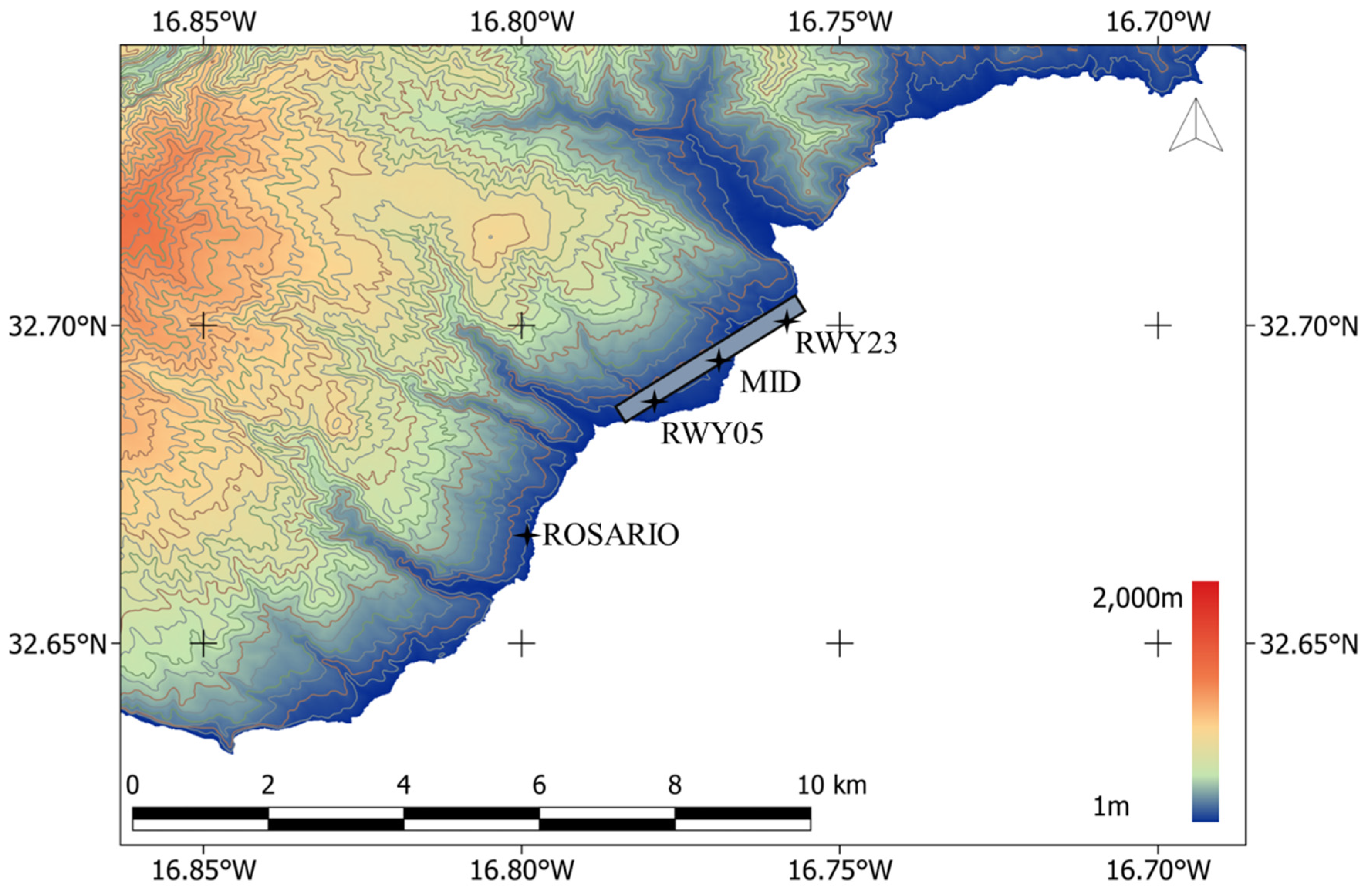
On the southeastern coast of Madeira, the largest island in the Madeira archipelago in the subtropical eastern North Atlantic, sits the Madeira International Airport, as shown in Figure 1. This unique geographic location presents a set of specific challenges due to the island’s complex topography, notably a significant mountain range. This characteristic significantly influences the climatic conditions at the airport, contributing to an intricate pattern of air flows and denoting substantial wind complexity, as the prevailing wind regime from the N and NE sectors is modified by the island topography [24,25].

The wind data utilized for this study are not publicly available, yet they were provided, upon request, by NAV Portugal E.P.E., a public corporate entity entrusted with the responsibility of providing air traffic services in Portugal.

Wind observations at Madeira Airport are recorded by a wind set from Väisälä, model WA15, comprised of a Väisälä Anemometer WAA151 and a Väisälä Wind Vane WAV151. This system is deployed in four different sites, one at the short-final of runway 05 (ROSARIO) and three others at different sectors of the airport: RWY05, MID, and RWY23, as illustrated in Figure 1. In their unprocessed form, collected data are captured every three seconds and stored on a server in a comma-separated values (CSV) format. This format includes a timestamp, the wind speed expressed in m/s, and the wind direction in degrees.

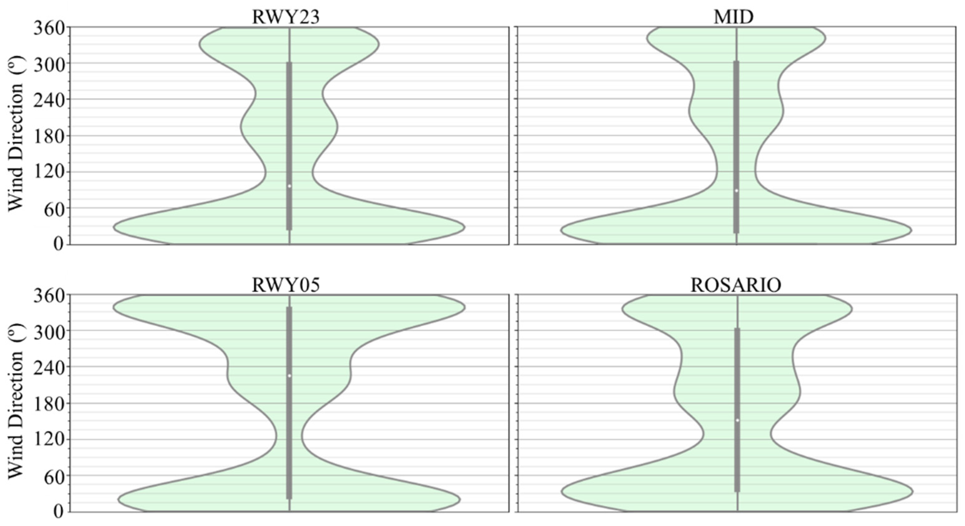
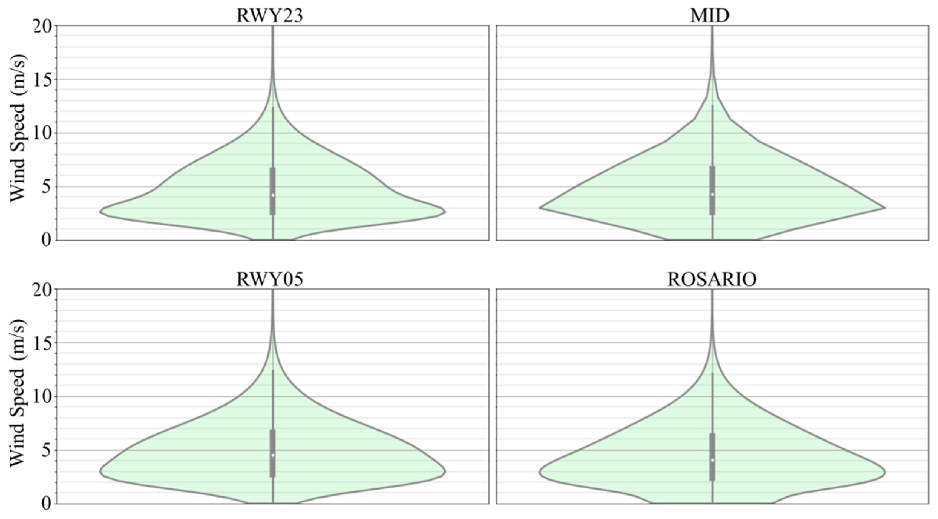
The provided dataset comprises complete CSV records collected from the four deployed sensors, covering the unprocessed three-second interval data for the years 2018 and 2019 and accounting for 84,096,000 potential observations, of which 84,040,836 contained valid and usable data. Figure 2 and Figure 3 display the distribution of the raw data for the entire period, showcasing the prevailing wind speed and direction for each sensor. It is noticeable that the predominant wind in the data occurs from the N and NE, averaging between 4.5 m/s and 4.9 m/s on ROSARIO and RWY05, respectively.

3.2. Methods

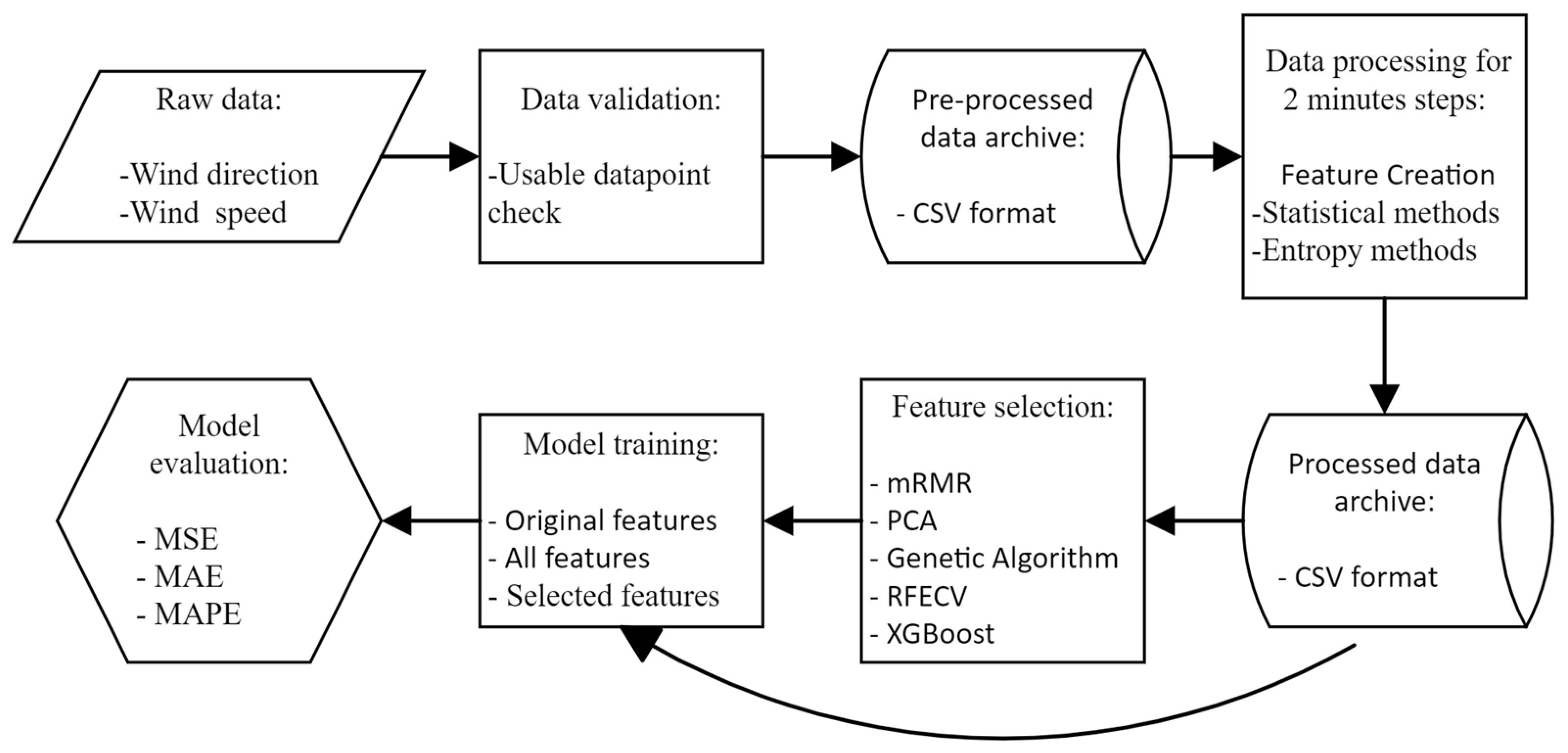
In this section, the research methodology employed is presented, emphasizing the major steps followed to analyze the more important features in wind nowcasting. The prediction process was based on feeding the model with the last 2 min of data for predicting the targeted 2 min, 10 min, and 20 min values, corresponding to the next step, 5 steps, and 10 steps of the dataset, respectively. Specifically, the 2 min and 10 min durations are defined by the World Meteorological Organization (WMO) for local and international wind reports, respectively, while the 20 min duration is drawn from the timeframes used in previous wind nowcasting studies [2,26,27]. A concise illustration of the stages followed in this work is provided in Figure 4.

3.2.1. Data Validation and Preprocessing

The raw data, composed of direct wind readings from each sensor, underwent a preprocessing phase via a Python algorithm to validate each three-second interval record. This step ensures valid readings for both wind speed and direction upstream, preventing issues during the rest of the process. Instances of missing or corrupted data were identified and discarded, resulting in a usable dataset consisting of 99.93% of the original raw data. Aligning with the WMO recommendation for local reports in aeronautical purposes, the raw data were subsequently reformatted into two-minute steps [2].

3.2.2. Data Processing and Feature Creation

After adjusting the time step, a mathematical approach encompassing standard statistical and entropy methods was employed for feature engineering, enabling the extraction of information, modification of existing features, and generation of new ones from the wind data to identify patterns and randomness for the subsequent stages of the study.

Features represent the quantifiable attributes or characteristics of the observed phenomena, serving as the variables that support the model’s decision-making or predictive capabilities. The process of feature engineering, which involves the generation of new features or modification of existing ones, encompasses a broad spectrum of transformations that can be applied to numerical data, such as mathematical approaches [28,29]. Consequently, 14 distinct features were derived, per sensor, totaling 56 features at a time resolution of two minutes.

Statistical Methods

The $\overrightarrow{u}$ and $\overrightarrow{v}$ wind components represent the west-to-east and south-to-north flows, respectively, and can be written as

$$\overrightarrow{u}=\frac{\sum _{i=1}^n\left[{-S}_i\times \sin \left(D_i\times \left(\frac{\pi }{180}\right)\right)\right]}{n}$$

(1)

$$\overrightarrow{v}=\frac{\sum _{i=1}^n\left[{-S}_i\times \cos \left(D_i\times \left(\frac{\pi }{180}\right)\right)\right]}{n}$$

(2)

where D is the wind direction in degrees, S is the wind speed in m/s, and n is the number of samples in the 2 min timestep [30,31,32].

Mean wind speed ($\overline{S}$) and direction ($\overline{D}$):

$$\overline{S}=\frac{\sum _{i=1}^n\left(S_i\right)}{n}$$

(3)

$$\overline{D}=\left(\arctan \left(\frac{\overrightarrow{u}}{\overrightarrow{v}}\right)+\mathsf{\pi }\right)\times \frac{180}{\mathsf{\pi }}$$

(4)

where $\overrightarrow{u} and \overrightarrow{v}$ are the mean 2 min wind components in m/s [30,31,32].

The wind speed maximum value, corresponding to the wind gust [27] (maxS) and standard deviation (stdS), can be calculated with

$$maxS={\max }_{\mathrm{i}=1}^{\mathrm{n}}\left(S_i\right)$$

(5)

$$stdS=\sqrt{\frac{{\sum }_{i=1}^n{\left(S_i-\overline{S}\right)}^2}{n-1}}$$

(6)

while the median (mdnS), if n is odd, is given by

$$smdnS={S_o}_{\left(\frac{n+1}{2}\right)}$$

(7)

and if n is even, it is defined as

$$smdnS=\frac{\left({S_o}_{\left(\frac{n}{2}\right)}+{S_o}_{\left(\frac{n}{2}+1\right)}\right)}{2}$$

(8)

where $S_o$ represents the wind speed values, in the interval, sorted from the lowest to the highest value [30,31,32].

Skewness (skwS) and kurtosis (krtS) provide insights into the shape and distribution, in addition to the symmetry and tail behavior of the wind data.

$$sskwS=\frac{1}{n}\sum _{i=1}^n{\left(\frac{S_i-\overline{S}}{\sqrt{\frac{{\sum }_{i=1}^n{\left(S_i-\overline{S}\right)}^2}{n-1}}}\right)}^3$$

(9)

$$krtS=\frac{1}{\mathrm{n}}\sum _{i=1}^n{\left(\frac{S_i-\overline{S}}{\sqrt{\frac{{\sum }_{i=1}^n{\left(S_i-\overline{S}\right)}^2}{n-1}}}\right)}^4$$

(10)

Entropy Methods

Shannon entropy (ShnE) measures the uncertainty or randomness of the data and can be calculated with

$$ShnE(S)=-\sum _{i=1}^n\mathrm{P}\left(S_i\right){\log }_2\mathrm{P}\left(S_i\right)$$

(11)

where P is the probability of occurrence, and S is the data values [33,34,35].

Sample entropy (SplE) is used to extract information about the complexity of the time-series data by quantifying the regularity and unpredictability of its fluctuations is given as

$$SplE\left(m\right)=-\ln \left(\frac{\mathrm{A}}{\mathrm{B}}\right)$$

(12)

where m is the embedding dimension, A is the number of template vectors of length m + 1 that are similar, and B is the number of template vectors of length m that are similar [33,35,36].

Multiscale entropy (MscE), which quantifies the complexity of the data over different timescales, is defined as

$$scE\left(m,r,\tau \right)=-\ln \left(\frac{\mathrm{A}\left(m,r,\tau \right)}{\mathrm{B}\left(m,r,\tau \right)}\right)$$

(13)

where m is the sequence length to compare, r is the maximum allowed difference for sequences to be considered similar, τ is the scale factor, and A and B are counts of similar sequences of lengths m + 1 and m, respectively [33,35,37].

Permutation entropy (PmtE) extracts the complexity of the data by examining all possible patterns or permutations and quantifying the pattern appearance in the defined time-steps and is given as

$$PmtE\left(m\right)=-\sum _{\mathsf{\pi }}\mathrm{p}\left(\mathsf{\pi }\right)\log \mathrm{p}\left(\mathsf{\pi }\right)$$

(14)

where π ranges over all m! possible permutations (m is the embedding dimension) of length m, and p is the normalized count of permutation [33,35,38].

Multiscale permutation entropy (MspE) is an extension of permutation entropy that takes into consideration multiple scales to analyze the complexity of the time series, allowing for the detection of features or complexities that might be invisible at the original scale but become evident when looking at larger scales, especially when the features manifest over multiple scales. It can be calculated with

$$MspE\left(m\right)=\left[PmtE\left(m,1\right),PmtE\left(m,2\right),\dots ,PmtE\left(m,{\tau }_{\max }\right)\right]$$

(15)

where PmtE was calculated with the coarse-grained time series at a particular scale τ, and the sequence 1, 2, …, ${\tau }_{\max }$ is the different scales at which the time series is coarse-grained and analyzed [33,35,39].

The feature engineering stage ended with a normalization process, which adjusted the range of each feature value between −1 and 1, fostering an equitable comparison between the features by mitigating potential scale disparities.

3.2.3. Feature Selection

Based on the state of the art, five feature selection techniques were chosen. The mRMR was chosen in alignment with the approach brought forth by Liu et al. [17], which emphasized mutual information-based feature selection. PCA was adopted, inspired by the work of Kong et al. [13], which effectively integrated it to identify influential factors affecting wind speed. RFECV was selected to consolidate the approach, emphasizing accuracy and efficiency, as noted in various studies [13,14,15,16,17,18,19,20,21]. The GA was employed due to its ability to emulate natural biological evolution processes, drawing parallels with the CRO method’s efficacy in identifying robust features. Lastly, XGBoost, as highlighted by Zha et al. [19], provided a compelling methodology for feature selection, leading to marked improvements in prediction accuracy metrics.

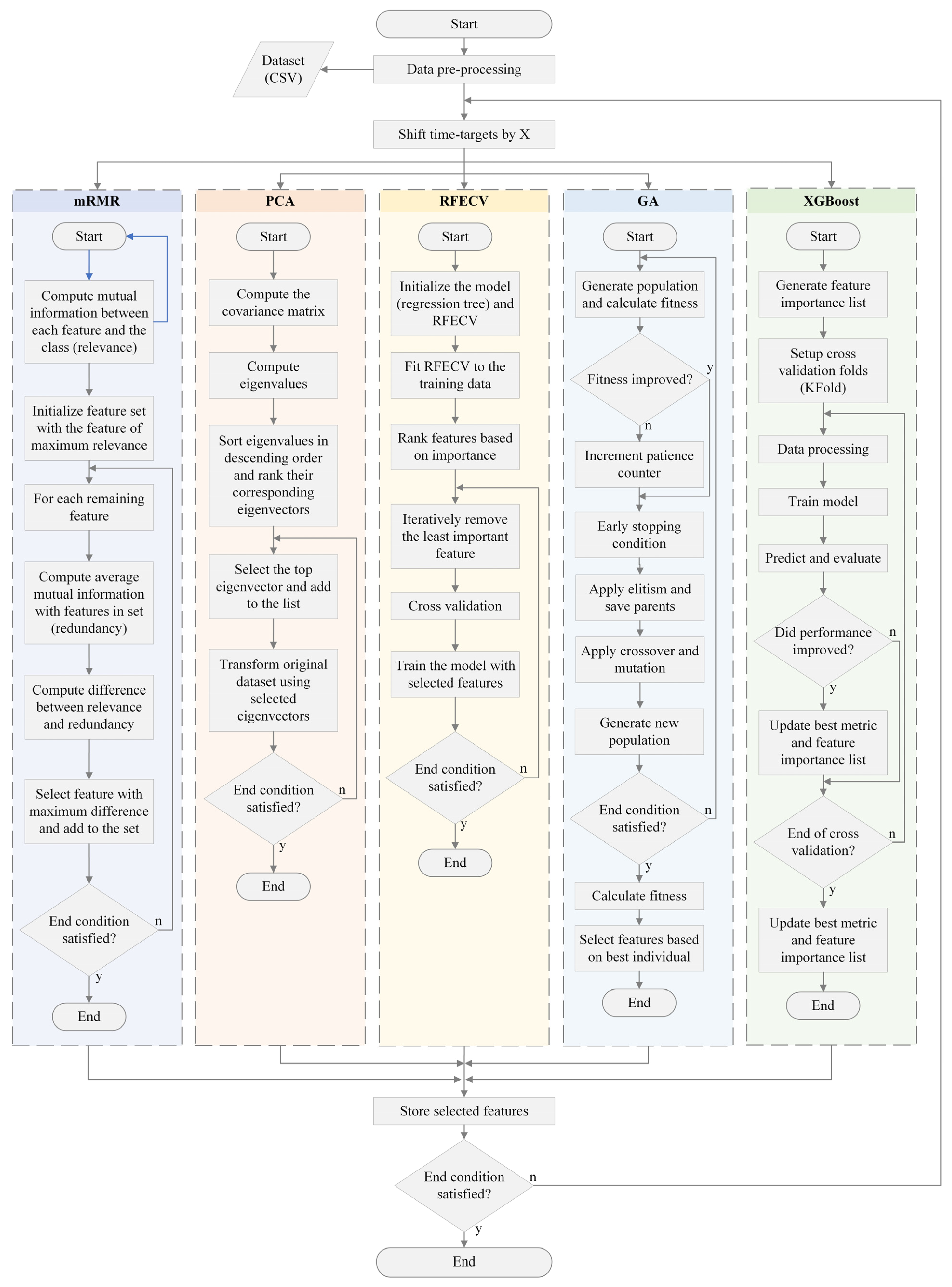
These techniques can be grouped into four broad feature selection categories: filter/dimensionality reduction, wrapper, and embedded methods [40]. In Figure 5, a flowchart is presented, which points to the steps and procedures followed in this process.

The feature selection process was carried out independently for each target variable and forecast window. This methodology was implemented to ensure an in-depth and varied understanding of the significance of each feature across distinct prediction scenarios. By isolating the process for every target variable and forecast window, variations in feature importance across different prediction variables and time horizons were discerned. Such an approach provides a comprehensive view, revealing how certain features might hold more importance for one prediction context but may wane in relevance in another.

The minimum redundancy maximum relevance (mRMR) and PCA techniques were employed as filter methods. The mRMR method, widely used for feature selection, brings inherent benefits, particularly its reduced computational complexity and processing speed. It works by selecting the features with high amounts of mutual information with the class but with minimum information shared between each other [41,42]. The PCA method is one of the classic and most widely used techniques to reduce the dimension of a dataset without losing statistical information [43,44]. The calculations were processed by Python 3 using pymrmr (version 0.1.11) and scikit-learn (version 1.2.2) libraries, and the number of features selected was based on the minimum mean absolute percentage error (MAPE) for each target and prediction window.

In wrapper methods, the recursive feature elimination with cross-validation (RFECV) and the Genetic Algorithm (GA), which is also considered an evolutionary search-based method, were used. A regression tree was chosen due to its quick processing speed, simplicity, minimal input parameters, which reduce subjectivity and enhance reproducibility, and its explainability potential, which lends itself to further exploratory studies [45,46,47,48,49,50].

Concerning the RFECV, a commonly used methodology that deletes features that may interfere with the result, data processing was performed using an algorithm that incorporated both the RFECV feature selection module and the decision tree regressor libraries, using a 5-fold cross-validation setup [51,52,53].

Regarding the GA, for optimization of the features involved, a Python script was developed to facilitate an evolutionary algorithm inspired by natural selection processes, emulating the process of natural biological evolution [54,55]. The developed GA optimizes the decision tree regressor’s feature selection using fitness scores derived from the MAPE and applied to a population of 100 individuals, in which each chromosomes had 56 genes. The fundamental mechanisms are the selection based on the best fitness individuals, multi-point crossover on reproducing steps, a mutation rate of 0.5%, and an early stopping criterion based on a lack of fitness improvement over ten generations.

Finally, the XGBoost embedded method was used. This feature-selection technique leverages a second-order Taylor expansion to approximate the loss function, enhancing model accuracy, and incorporates a regular term to control model complexity, thereby preventing overfitting. It employs feature importance selection, an embedded method, wherein gain is used to identify optimal segmentation nodes during training. The importance of each feature is gauged by calculating the average gain (total gain of all trees divided by each feature’s division count), which indicates the feature’s contribution to the model’s construction and training. Therefore, XGBoost is an optimal choice for wind feature selection since its integrated regularization can prevent overfitting and demonstrates its efficient cross-validation implementation for accurate assessment [56,57,58].

For feature selection, the mRMR method employed the Mutual Information Quotient (MIQ) from the pymrmr library, while the GA relied on the mean absolute percentage error (MAPE). The RFECV, as defined by the default values in scikit-learn, utilized the R² score for evaluation. XGBoost determined feature importance through gain during its training process.

To prevent overfitting, scikit-learn’s regression tree and XGBoost’s specific default parameters were used. For scikit-learn’s regression tree, nodes are expanded until all leaves contain fewer than the default value of minimum samples split, which is set to 2. In XGBoost, the subsample parameter defaults to 1, indicating that the model uses the entire dataset, and the learning rate (or eta) is set to 0.3. These inherent parameter settings mitigate the risk of overfitting, thus helping the models generalize effectively to unseen data.

3.2.4. ML Model Training

An ML model was trained using the selected features from each selection technique and the set of all created features. A low-complexity regression tree model was chosen due to its utility in systematically classifying outputs based on low input parameters that enable the reduction of parameter range based on objective criteria and aid in establishing relationships from input data to the end results [50].

Regression trees, a variant of decision tree models, are adept at processing continuous data by partitioning the dataset into homogeneous groups at specific nodes, each representing a decision point based on an independent variable, and the final partitions condense the outcome as a continuous value [48]. Regression trees can also discern variables’ importance within a dataset. Still, this local optimization can prioritize background variables with significant indirect effects over those directly influencing the response [49], hence the usage and feature selection techniques to ensure proper feature assortment.

The model training phase utilized seven distinct feature sets, each representing the output of various feature selection processes. Five of these sets were derived from separate individual selection processes, while, alongside, an encompassing set was created incorporating all the variables that were produced. A control set was also established, containing solely the original dataset wind variables—wind speed, direction, and gust, at a 2-min timestep. Each of these sets corresponds to the features chosen through their respective selection methods. Consequently, seven corresponding models were developed, each representing the unique characteristics of its respective feature set.

All models were trained using the mean squared error (MSE) as the evaluation metric. For the XGBoost model, the default hyperparameters from scikit-learn version 1.3.0 were employed. The parameters encompassed a learning rate set to 0.3, a number of estimators set to 100, a maximum depth set to 6, a subsample value set to 1, a column sample by tree set to 1, and the objective set as ‘reg:squarederror’.

3.2.5. ML Model Evaluation

To evaluate each trained model, a comparative analysis was employed to identify the best set of features and the selection technique that delivered superior results. The assessment was performed using MAE, MSE, and MAPE as evaluation and comparison metrics [59]. These metrics are defined as

$$MAE=\frac{1}{m}\sum _{i=1}^m\left|X_i-Y_i\right|$$

(16)

$$MSE=\frac{1}{m}\sum _{i=1}^m{\left(X_i-Y_i\right)}^2$$

(17)

$$MMAPE=\frac{1}{m}\sum _{i=1}^m\left|\frac{|X_i-Y_i}{Y_i}\right|$$

(18)

For the feature selection and training procedures, all the data from the years 2018 and 2019 were used with a 5-fold cross-validation approach to ensure statistical robustness and mitigate the risk of overfitting in the model’s predictions. The shuffling procedure divided the dataset into five distinct folds, with each fold serving as a testing set rotationally, whereas the remaining folds formed the training set. While not directly ensuring statistical relevance, this method facilitated the assessment of the model’s performance across different data subsets, thereby reducing overfitting and improving the generalizability of the model’s results [60].

The three assessed targets were the subsequent 2, 10, and 20 min for the MID sensor, as this sensor is considered the most important in the airport.

4. Results

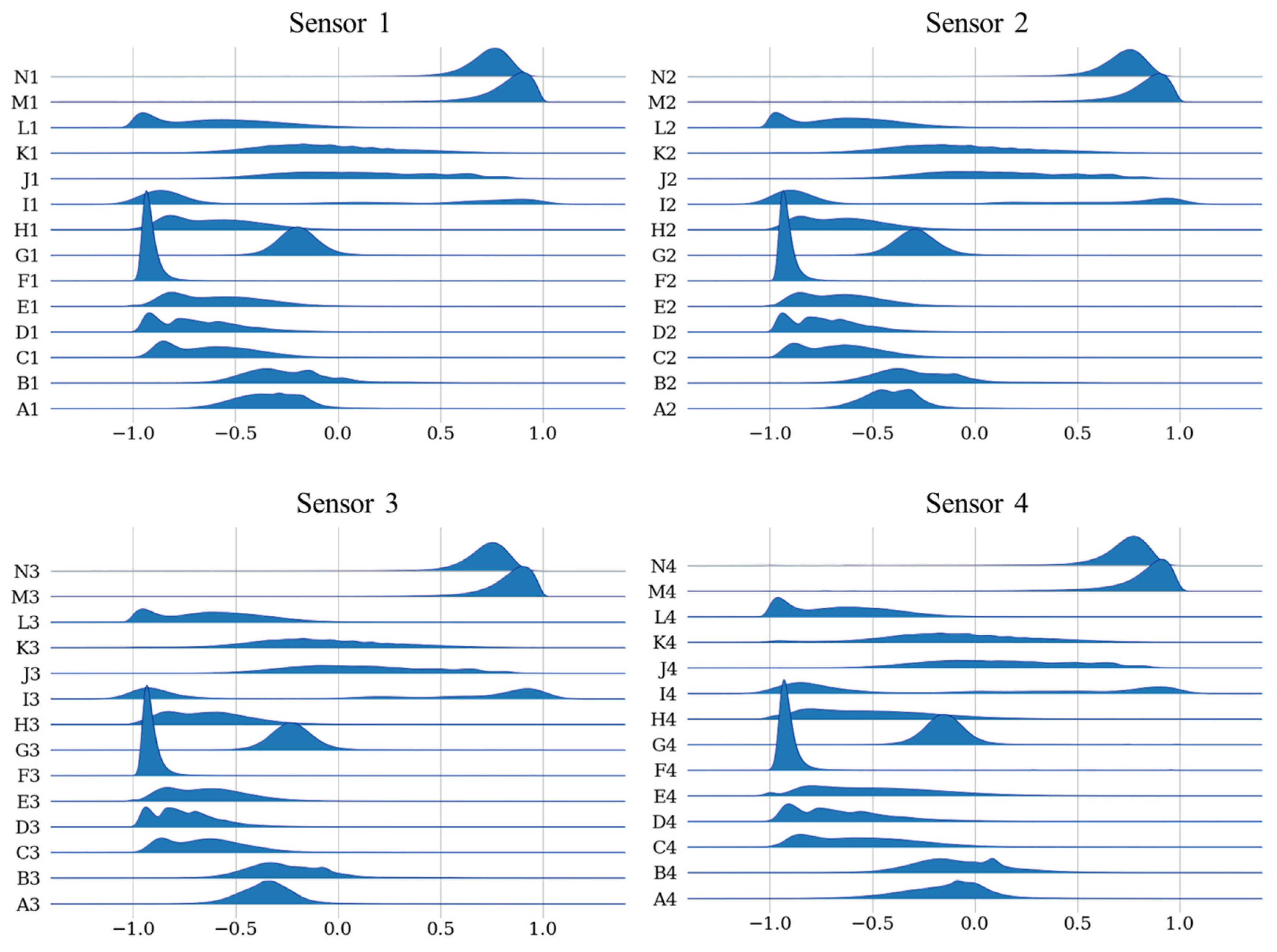
This section presents the attained results. After the preprocessing and feature creation steps, 14 distinct variables were computed for each sensor, aggregating to 56 features. For each sensor, the 14 derived features—[Wind U Component, Wind V Component, Maximum Instant Wind Speed, Wind Speed Standard Deviation, Wind Speed Median, Wind Speed Kurtosis, Wind Speed Skewness, Mean Wind Speed, Mean Wind Direction, Shannon Entropy, Sample Entropy, Multiscale Entropy, Permutation Entropy, and Multiscale Permutation Entropy]—are further denoted by the sequence [An, Bn, Cn, Dn, En, Fn, Gn, Hn, In, Jn, Kn, Ln, Mn, Nn], where n corresponds to the sensor number [1,2,3,4], matching positions RWY23, MID, RWY05, and ROSARIO, respectively. Figure 6 presents the data distribution from all sensors and features.

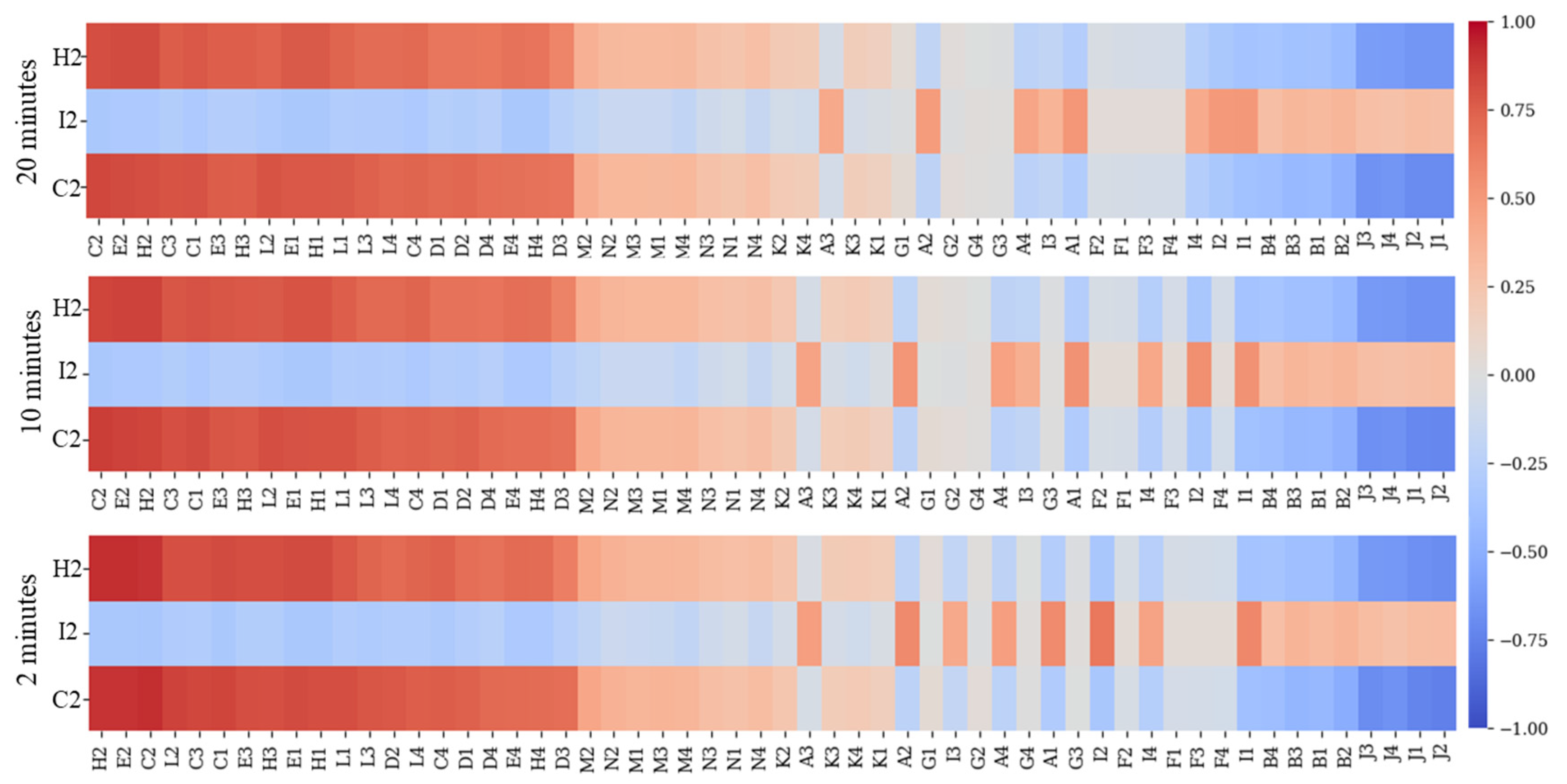
Figure 7 presents the Pearson correlation coefficient for each target feature at all studied forecast windows, sorted from left to right by the highest mean correlation value, showing strong correlation between sensors.

Table 1. Selected features by algorithm. S, D, and G correspond to speed, direction, and gust, respectively.

Algorithm	Time	Target	Features
mRMR	2	Speed	E1 E2 E3 E4 J2 J3 L1 L2 L3 L4
		Direction	E1 E2 E3 E4 I2 J2 L1 L2 L3 L4
		Gust	C1 E1 E2 E3 E4 H1 L1 L2 L3 L4
	10	Speed	E1 E2 E3 E4 J2 J3 L1 L2 L3 L4
		Direction	E1 E2 E3 E4 J2 J3 L1 L2 L3 L4
		Gust	E1 E2 E3 E4 J2 J3 L1 L2 L3 L4
	20	Speed	E1 E2 E3 E4 J2 J3 L1 L2 L3 L4
		Direction	E1 E2 E3 E4 J2 J3 L1 L2 L3 L4
		Gust	E1 E2 E3 E4 J2 J3 L1 L2 L3 L4
GA	2	Speed	A1 A2 A3 B4 C1 D1 D2 D4 E3 E4 F2 F4 G1 G2 H1 H2 H3 H4 I2 J2 J4 K3 L1 M1 N1 N4
		Direction	A2 A3 A4 B4 C2 C3 C4 D3 D4 E3 F2 F4 G1 G2 G3 I2 I3 I4 J2 J4 K1 K2 L1 M2 M3 N1 N2
		Gust	A2 A4 B2 B3 B4 C1 C2 C4 D1 D2 D3 D4 E3 F2 F3 G1 H1 H2 I3 I4 J2 J3 J4 L3 L4 M1 M3 N1
	10	Speed	A1 A4 B1 B2 B3 C4 D1 D2 E1 E2 E3 F1 F3 F4 G1 G2 G3 H2 I1 J1 K1 K2 K3 L1 L4 M1 M3 N1 N2 N4
		Direction	A1 A3 B3 C2 C3 C4 D2 F3 F4 G3 G4 H1 I2 J1 J3 J4 K1 K2 K3 K4 L4 M1 M3 N1 N3 N4
		Gust	A1 A2 A4 B2 B3 C2 C4 D2 E1 E4 F1 F3 G1 G2 G3 H2 H3 I1 I2 J1 J3 J4 K4 L2 L3 L4 M2 M4
	20	Speed	A1 A2 A4 B1 B3 B4 C1 C3 D1 D3 D4 E2 E3 F2 F4 G1 H2 I1 I3 I4 J1 J2 K1 K2 K4 L1 L2 L4 M1 M2 N3 N4
		Direction	A1 A3 B1 B2 B3 B4 C1 C4 D1 D3 E2 E4 F1 F3 F4 G1 H1 I1 I2 I4 K1 K3 L1 L3 M3 N3
		Gust	A1 A2 A3 A4 B1 B2 C1 C3 D1 D2 D3 E1 E2 E3 E4 F1 F3 F4 G3 G4 H1 I1 I4 J2 J3 J4 K1 K2 K3 K4 L1 L2 L3 M1 M4
XGBoost	2	Speed	A2 A3 B2 C2 E2 H2 I1 I2 I3 I4
		Direction	A2 A3 B2 C2 E2 H2 I1 I2 I3 I4
		Gust	A2 A3 B2 C2 E2 H2 I1 I2 I3 I4
	10	Speed	A1 A2 A3 C2 H2 H3 I1 I2 I3 I4
		Direction	A1 A2 A3 C2 H2 H3 I1 I2 I3 I4
		Gust	A1 A2 A3 C2 H2 H3 I1 I2 I3 I4
	20	Speed	A1 A2 A3 A4 C2 H2 H3 I1 I2 I4
		Direction	A1 A2 A3 A4 C2 H2 H3 I1 I2 I4
		Gust	A1 A2 A3 A4 C2 H2 H3 I1 I2 I4
RFECV	2	Speed	A1 A2 A3 B3 B4 C2 D3 H2 I1 I2 I4 L1
		Direction	A1 A2 A3 B3 B4 C2 D3 G1 H2 I1 I2 I3 I4 L1
		Gust	A1 A2 A3 B3 C2 D3 F4 H2 I1 I2 I4 L1
	10	Speed	A1 A3 A4 B1 B3 B4 C2 D3 H2 I1 I2
		Direction	A1 A2 A3 A4 B1 B3 B4 C2 D1 D3 G4 H2 I1 I2 I3 I4 L2 N3
		Gust	A1 A3 A4 B1 B3 B4 C2 D3 H2 I1 I2
	20	Speed	A1 A2 A3 A4 B1 B2 B3 B4 C1 C2 C3 C4 D1 D2 D3 D4 E1 E2 E4 F1 F2 F3 F4 G1 G2 G3 G4 H1 H2 H3 H4 I1 I2 I3 I4 J1 J2 J3 J4 K1 K2 K3 K4 L1 L2 L3 L4 M1 M2 M3 M4 N1 N2 N3 N4
		Direction	A1 A2 A3 A4 B1 B2 B3 B4 C1 C2 C3 C4 D1 D2 D3 D4 E1 E2 E4 F1 F2 F3 F4 G1 G2 G3 G4 H1 H2 H3 H4 I1 I2 I3 I4 J1 J2 J3 J4 K1 K2 K3 K4 L1 L2 L3 L4 M1 M2 M3 M4 N1 N2 N3 N4
		Gust	A1 A2 A3 A4 B1 B2 B3 B4 C1 C2 C3 C4 D1 D2 D3 D4 E1 E2 E4 F1 F2 F3 F4 G1 G2 G3 G4 H1 H2 H3 H4 I1 I2 I3 I4 J1 J2 J3 J4 K1 K2 K3 K4 L1 L2 L3 L4 M1 M2 M3 M4 N1 N2 N3 N4
PCA	2	Speed	F1 F2 F3 F4 F5 F6 F7 F8 F9 F10 F11 F12 F13
		Direction	F1 F2 F3 F4 F5 F6 F7 F8 F9 F10 F11 F12 F13 F14 F15 F16 F17 F18 F19 F20
		Gust	F1 F2 F3 F4 F5 F6 F7 F8 F9 F10 F11 F12 F13 F14 F15 F16 F17 F18 F19 F20
	10	Speed	F1 F2 F3 F4 F5 F6 F7 F8 F9 F10 F11 F12 F13 F14
		Direction	F1 F2 F3 F4 F5 F6 F7 F8 F9 F10 F11 F12 F13 F14 F15 F16 F17 F18 F19 F20 F21 F2
		Gust	F1 F2 F3 F4 F5 F6 F7 F8 F9 F10 F11 F12 F13 F14 F15 F16 F17 F18 F19 F20 F21
	20	Speed	F1 F2 F3 F4 F5 F6 F7 F8 F9 F10 F11 F12 F13 F14 F15 F16 F17 F18 F19 F20 F21
		Direction	F1 F2 F3 F4 F5 F6 F7 F8 F9 F10 F11 F12 F13 F14 F15 F16 F17 F18 F19 F20
		Gust	F1 F2 F3 F4 F5 F6 F7 F8 F9 F10 F11 F12 F13 F14 F15 F16 F17 F18 F19

depicts all the features selected by each technique for all time targets.

Table 2. Wind speed nowcast performance metrics, presenting the results, as mean ± standard deviation, for the three forecasted time targets. The lowest error for each period is highlighted in bold.

Target H2	2 min			10 min			20 min
Set	MSE	MAE	MAPE	Set	MSE	MAE	MAPE	Set	MSE
Control	1.90	1.00	0.36	3.15	1.32	0.55	3.92	1.48	0.64
	±0.02	±<0.01	±0.02	±0.02	±<0.01	±0.03	±0.03	±<0.01	±0.02
All	1.88	1.00	0.35	3.15	1.32	0.55	3.91	1.48	0.64
	±0.01	±<0.01	±0.01	±0.01	±<0.01	±0.01	±0.04	±0.01	±0.03
mRMR	2.01	1.04	0.37	3.33	1.36	0.56	4.12	1.52	0.67
	±0.01	±<0.01	±0.02	±0.04	±0.01	±0.01	±0.02	±<0.01	±0.03
PCA	1.96	1.03	0.37	3.12	1.31	0.53	3.87	1.47	0.63
	±0.03	±0.01	±0.01	±0.03	±<0.01	±0.01	±0.03	±<0.01	±0.02
RFECV	1.90	1.00	0.35	3.11	1.31	0.54	3.90	1.48	0.63
	±0.02	±<0.01	±0.01	±0.02	±<0.01	±0.01	±0.03	±0.01	±0.03
GA	1.90	1.01	0.36	3.19	1.33	0.55	3.89	1.48	0.64
	±0.01	±<0.01	±0.01	±0.02	±<0.01	±0.02	±0.03	±<0.01	±0.03
XGBoost	2.07	1.05	0.37	3.27	1.35	0.56	3.98	1.49	0.65
	±0.02	±<0.01	±0.02	±0.02	±<0.01	±0.03	±0.03	±<0.01	±0.03

,

Table 3. Wind direction nowcast performance metrics, presenting the results, as mean ± standard deviation, for the three forecasted time targets. The lowest error for each period is highlighted in bold.

Target I2	2 min			10 min			20 min
Set	MSE	MAE	MAPE	MSE	MAE	MAPE	MSE	MAE	MAPE
Control	1.75 × 104	63.58	2.91 × 1013	2.18 × 104	81.30	3.63 × 1013	2.37 × 104	89.58	3.19 × 1013
	±1.55 × 102	±0.46	±2.62 × 1013	±1.43 × 102	±0.43	±3.10 × 1013	±2.84 × 102	±0.83	±3.23 × 1013
All	1.77 × 104	64.61	3.48 × 1013	2.20 × 104	82.50	4.02 × 1013	2.40 ×104	90.79	3.36 × 1013
	±1.92 × 102	±0.55	±2.50 × 1013	±2.57 × 102	±0.74	±3.39 × 1013	±1.38 × 102	±0.41	±3.61 × 1013
mRMR	1.87 × 104	67.69	1.09 × 1013	2.98 × 104	114.68	3.51 × 1013	3.04 × 104	117.10	3.49 × 1013
	±1.49 × 102	±0.48	±1.43 × 1013	±1.79 × 102	±0.49	±3.48 × 1013	±2.63 × 102	±0.87	±3.29 × 1013
PCA	1.85 × 104	68.26	2.32 × 1013	2.22 × 104	82.95	2.69 × 1013	2.41 × 104	90.97	1.80 × 1013
	±1.36 × 102	±0.33	±2.06 × 1013	±9.31 × 101	±0.20	±1.53 × 1013	±1.60 × 102	±0.48	±1.42 × 1013
RFECV	1.74 × 104	63.53	3.56 × 1013	2.18 × 104	81.49	3.39 × 1013	2.40 × 104	90.84	3.27 × 1013
	±1.43 × 102	±0.45	±2.22 × 1013	±1.77 × 102	±0.48	±3.18 × 1013	±1.03 × 102	±0.33	±3.77 × 1013
GA	1.80 × 104	65.48	2.63 × 1013	2.25 × 104	84.19	3.21 × 1013	2.41 × 104	90.97	4.01 × 1013
	±3.42 × 101	±0.07	±2.51 × 1013	±2.36 × 102	±0.68	±3.04 × 1013	±1.59 × 102	±0.49	±4.04 × 1013
XGBoost	1.76 × 104	63.78	3.30 × 1013	2.18 × 104	81.50	3.28 × 1013	2.38 × 104	90.04	3.10 × 1013
	±9.31 × 101	±0.29	±1.90 × 1013	±1.23 × 102	±0.36	±2.69 × 1013	±1.47 × 102	±0.49	±3.40 × 1013

and

Table 4. Wind gust nowcast performance metrics, presenting the results, as mean ± standard deviation, for the three forecasted time targets. The lowest error for each period is highlighted in bold.

Target C2	2 min			10 min			20 min
Set	MSE	MAE	MAPE	Set	MSE	MAE	MAPE	Set	MSE
Control	3.47	1.34	0.24	5.35	1.70	0.33	6.45	1.89	0.38
	±0.01	±<0.01	±<0.01	±0.04	±0.01	±<0.01	±0.06	±0.01	±<0.01
All	3.43	1.33	0.24	5.27	1.69	0.33	6.44	1.89	0.38
	±0.01	±<0.01	±<0.01	±0.05	±0.01	±<0.01	±0.04	±0.01	±<0.01
mRMR	3.63	1.37	0.24	5.55	1.75	0.34	6.81	1.95	0.40
	±0.04	±<0.01	±<0.01	±0.05	±0.01	±<0.01	±0.07	±0.01	±<0.01
PCA	3.64	1.38	0.25	5.36	1.71	0.33	6.53	1.90	0.38
	±0.02	±<0.01	±<0.01	±0.03	±<0.01	±<0.01	±0.04	±<0.01	±<0.01
RFECV	3.52	1.35	0.24	5.34	1.70	0.33	6.44	1.89	0.38
	±0.01	±<0.01	±<0.01	±0.03	±<0.01	±<0.01	±0.05	±0.01	±<0.01
GA	3.46	1.34	0.24	5.34	1.70	0.33	6.50	1.90	0.38
	±0.02	±<0.01	±<0.01	±0.03	±<0.01	±<0.01	±0.02	±0.01	±<0.01
XGBoost	3.93	1.42	0.25	5.66	1.75	0.34	6.76	1.93	0.39
	±0.04	±0.01	±<0.01	±0.04	±0.01	±<0.01	±0.05	±0.01	±<0.01

present an in-depth overview of the results for each evaluated metric and feature for wind speed, wind direction, and wind gust targets, respectively. The presented results refer to the test dataset, where a standard tree was trained with the features selected by the feature selection methods and then evaluated on the independent test data.

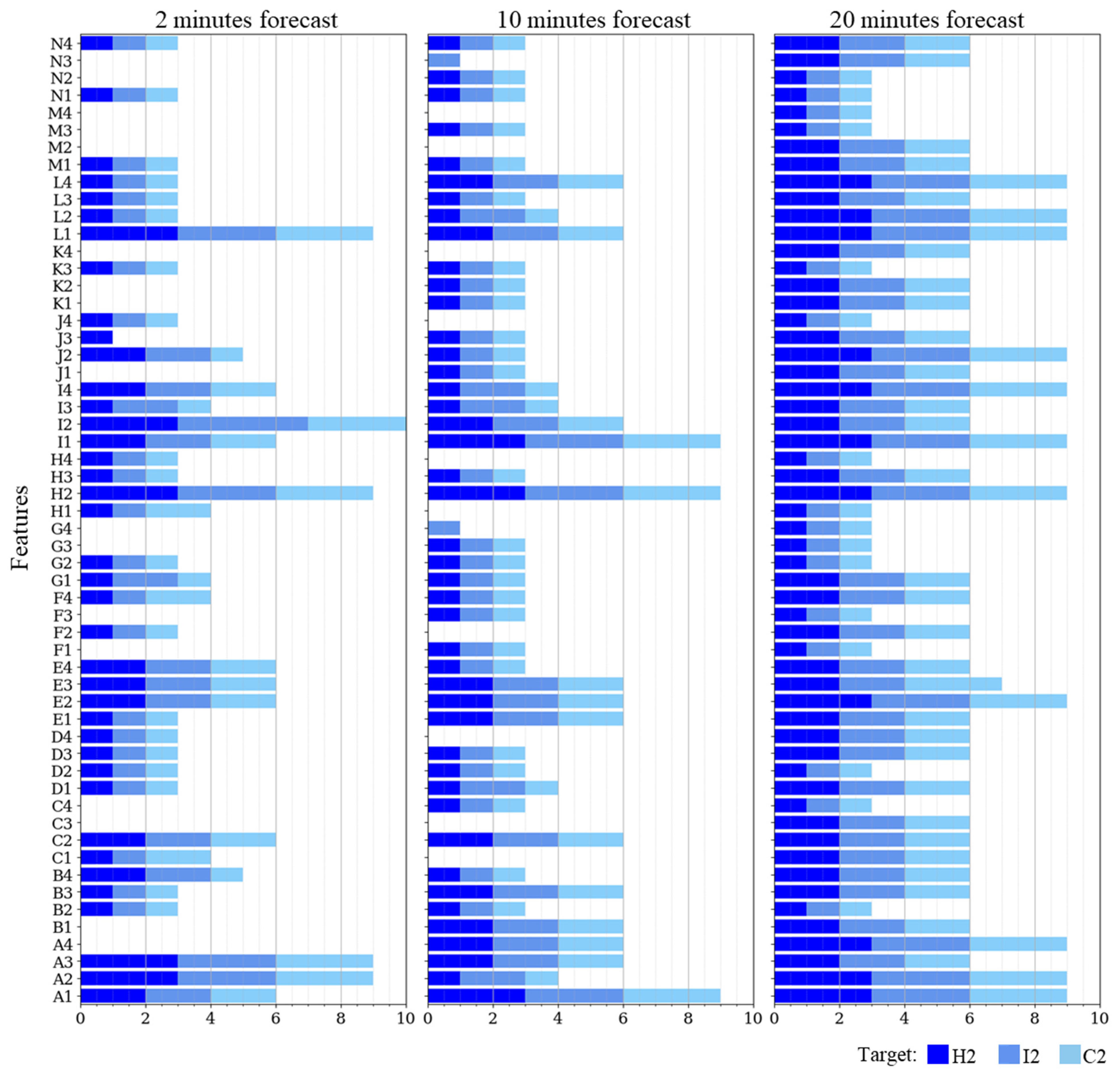
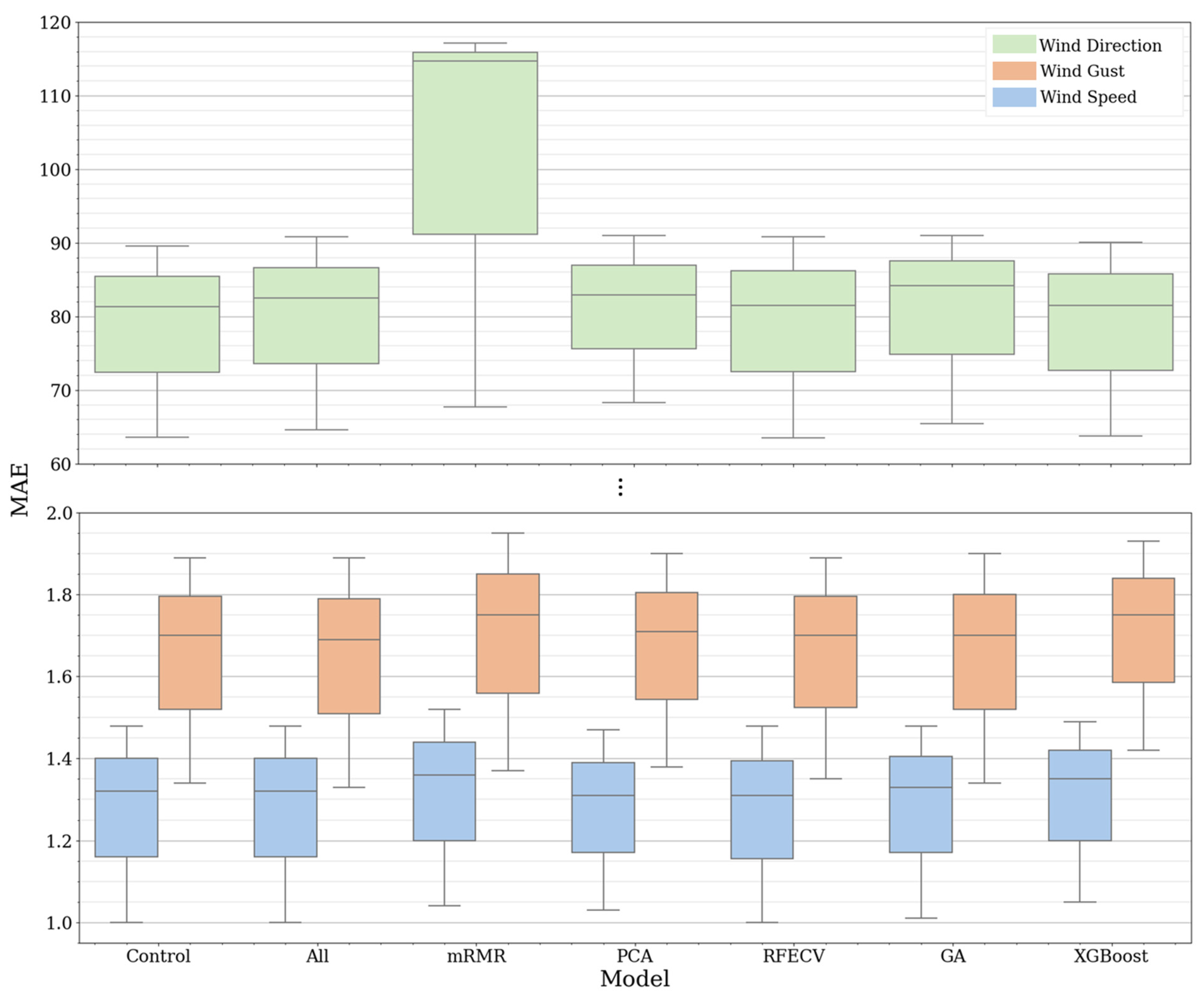
Figure 8 illustrates the frequencies of feature choice by the feature selection methods. The figure displays the number of times each feature was selected for individual target variables and the cumulative occurrence. Figure 9 depicts the performance of the model for each selection process, highlighting the features used. The model’s efficiency is gauged using the mean absolute error (MAE) as a reference metric across all forecasted periods.

5. Discussion

This research offers an extensive examination of wind nowcasting, focusing on the role of nowcast duration and feature selection in predictive model performance. Our findings underscore the complexity of wind prediction as the nowcast horizon extends, as evidenced by the rising error values between 2 min and 20 min prediction window. This complexity stems from the inherent variability and nonlinearity of wind speed and direction, which increase as the prediction window expands. Furthermore, the higher prediction errors for the mean wind direction highlight the intricate atmospheric dynamics that influence wind direction and the associated challenge for machine learning models in predicting this variable.

Based on Table 2, Table 3 and Table 4, when forecasting wind speeds and directions, distinct patterns become evident over the different time horizons. For the mean wind speed, the 2 min forecast presents the narrowest discrepancy between methods, with MAE values oscillating between 1.00 (All methods) and 1.05 (XGBoost). Extending the prediction horizon to the 10 min forecast reveals that mRMR exhibits the most substantial deviation, with an MAE of 1.36, while RFECV registers the lowest error at 1.31. At the 20 min mark, the variations are more pronounced, with values spanning from 1.46 (PCA) to 1.52 (mRMR). For the wind direction mean, the 2 min forecast sees MAE values ranging from 63.53 (RFECV) to 68.26 (PCA). This discrepancy broadens at the 10 min forecast, with RFECV at the lower end registering an MAE of 81.30, and mRMR at the top with a significant 114.68. This trend persists into the 20 min forecast, where MAE values fluctuate between 89.58 (control) and 117.10 (mRMR). Lastly, for the wind gust, the 2 min predictions range between 1.33 (all method) and 1.42 (XGBoost). For the 10 min forecast, RFECV shows the least MSE at 1.70, while mRMR records an error of 1.75. For the 20 min predictions, the error for mRMR peaks at 1.95, contrasting with the all method’s more modest 1.89. Overall, predictions for wind speed are relatively consistent across the methods implemented, but predictions for wind direction exhibit more variability as the forecasting window extends.

Therefore, the impact of feature creation and selection on model performance emerged as a significant aspect of this study. Our results suggest that generating wind features mathematically may enhance predictive accuracy and reduce computational requirements. Indeed, our research revealed that for wind speed nowcast, the fewer features selected through RFECV and PCA not only maintained but improved prediction accuracy, hinting at opportunities for computational optimization. However, when examining the wind direction nowcast, it is clear that the errors are immense due to two factors, specifically, the large range of the values, varying from 1° to 360°, and the variations at the border between 360° and 1°. (For example, when the model forecasted the direction to be 1°, but the ground truth label was 360°, it leads to an error of 359°, enlarging the error metrics, but in reality, the error is just 1°.) It is also crucial to consider the complex wind patterns in the studied location, where the wind can be considerably turbulent with fast direction variation. Lastly, the gust nowcast error was lower in the methods that used more features, stressing the importance of the additional information provided by the features.

The marginal improvements in nowcast accuracy achieved through advanced feature creation and selection techniques require a careful analysis of the trade-off between the computational cost and the predictive performance. Upon further examination of the results, it was observed that the 14 engineered features per sensor did not yield a notable enhancement in model accuracy. The slight variations in metrics across different feature selection methods suggest that while some methods might yield minor improvements for certain metrics, they may not always ensure superior performance across all metrics and time intervals.

In Figure 8, it is noteworthy that overall, nine features were selected more than 20 times (I2, I1, H2, A3, A2, A1, C2, L1, I4), and seven other features were selected more than 15 times (E2, L4, J2, E4, E3, L2, L3). The most selected feature, with 24 occurrences, was I2, while the least selected, with four incidences, was H4. The control set of features contained 12 features for each target and nowcasted time, while the group with all features contained 56. The mRMR and XGBoost methods each selected ten features for every target and projected time. When considering the two-minute nowcast, the GA method’s feature selection varied depending on the target: 26 for H2, 27 for I2, and 28 for C2. In the case of the ten-minute nowcast, the feature selections for each respective target were 30, 26, and 28, respectively. Lastly, the chosen features numbered 32, 26, and 35, respectively, for the most extended nowcast period. In a similar pattern, RFECV opted for 12, 14, and 12 features, respectively, for the first set, and 11, 14, and 18, respectively, for the second set. For the longest prediction interval, it utilized nearly all the features, specifically 55, 55, and 56. For PCA, the number of features was 20, 20, and 13, respectively, for the 2 min forecast, while it was 14, 22, and 21, respectively, for the 10 min and 21, 20, and 19 for the 20 min prediction, for H2, I2, and C2 target, respectively. It is also renowned that, in general, as the forecasted time increases (from 2 to 20 min), the number of selected features also increases, suggesting that the additional information of the less relevant features becomes progressively more relevant to provide context.

The salient outcome of this study highlights a pronounced spatial correlation among sensors located at variable distances from the intended prediction point, which corresponded to the middle of the runway, at the position of the MID wind sensor. Figure 7 extrapolates this correlation, providing computational details between each feature, target, and prediction timeframe, particularly underscoring the strong correlation of features from sensors such as C1, E3, H3, and E1, which rank within the top 10. An illustration of these findings can also be seen in Figure 6, where the individual sensor features demonstrate distinct intra-sensor distributions but exhibit similarity when compared to features across other sensors, emphasizing a robust sensor intercorrelation. This correlation is further supported by Figure 8, indicating the selection of features from diverse sensors across all prediction targets and windows.

In conjunction with the observed fluctuations in feature importance across different nowcast durations, this correlation underscores the significance of the spatial-temporal context in enhancing prediction precision. This understanding augments our capacity to discern intricate spatial patterns in wind behavior, thereby harboring the potential to optimize wind nowcast models over various time spans.

Table 5. State-of-the-art analysis for feature selection for wind speed forecast.

Work	Time Resolution	FS Methods	Data	Performance
Salcedo-Sanz et al. [12]	10 min	CRO	1 year	MSE 2.50
Kong et al. [13]	More than 1 h	PCA-based	1 month	MAE 0.20, MAPE 0.05, and RMSE 0.45
Paramasivan and Lopez [14]	15 min	Relief	1 month	MSE 0.48
Zhang et al. [15]	1 h	Empirical mode decomposition	1 month	MAE 0.60, MAPE 13.30, and RMSE 0.79
Feng et al. [16]	1 h	Deep feature selection	1 year	NMAE 3.76 and NRMSE 5.21
Liu et al. [17]	10 min	Mutual information based	9 months	MAE 0.31, MAPE 7.13, and RMSE 0.39
Mir et al. [18]	10 min	Hybrid feature selection	3 years	MAE 0.47
Zha et al. [19]	15 min	XGBoost based	6 months	-
El-kenawy et al. [20]	1 h	ADGWDTO	-	MAE 0.002 and RMSE 0.003
Lv and Wang [21]	1 h	FWNSDEC-SSA	1 year	MAE 0.04, MAPE 1.09, and RMSE 0.07
This work	2 min	mRMR, PCA, RFECV, GA and XGBoost	2 years	MAE 1.00, MAPE 0.35, and MSE 1.90

provides a comprehensive comparison of the wind speed forecasting methodology against existing state-of-the-art approaches. Notably, only the study by Liu et al. [17] spanned a longer duration than this study. However, the current work boasts a time resolution that is five times finer, and its performance metrics remain comparable, underscoring the significance and robustness of the methodology. Many of the referenced studies utilized considerably shorter timeframes, potentially limiting their ability to discern synoptic wind patterns effectively.

In terms of performance, the results from the current research align well with the prevailing state of the art, even with the enhanced resolution and higher data volume. A distinctive feature of this approach is the incorporation of feature creation, a technique not deeply observed in other studies. Moreover, the selection methods resonate with the best practices in the field. It is also worth noting that this research was the only one, to the best of the authors’ knowledge, that focused on wind gust and direction using feature engineering.

Considering these findings, it becomes clear that the considerations of nowcast duration, feature selection, computational cost-benefit trade-offs, and spatial-temporal interrelationships are paramount in wind nowcasting. While advanced mathematical features and machine learning models show promise, their application should be carefully evaluated on a case-by-case basis due to the associated computational costs. Importantly, recognizing and leveraging spatial correlations present a promising pathway for enhancing the accuracy and reliability of wind nowcasting, an element vital for the operational efficiency of wind-dependent systems and industries.

6. Conclusions

This work explores the intricacies of wind nowcasting, contributing to meteorological studies and the domain of computational modeling. The investigation proved the escalated challenges when extending nowcast horizons, evidenced by the surge in error values from a 2 min to a 20 min prediction window. This trend results from the inherent variability and nonlinearity of wind speed and direction, which become increasingly conspicuous over extended durations. Furthermore, the discrepancy in error rates between mean wind direction and other parameters underlines the intricate, atmospheric dynamics influencing wind direction, showing ML models’ increased difficulty in predicting this variable.

A key facet of this study was the emphasis on feature creation and selection and determining the efficacy of the resulting prediction models. The data suggest that the mathematical generation of wind features could slightly enhance predictive accuracy. Notably, the research demonstrated that a reduction in features, through feature selection methods, in certain instances, did not compromise accuracy but improved it, implying potential avenues for optimizing computational efficiency.

Nonetheless, the marginal enhancement in nowcast accuracy through advanced feature creation and selection mechanisms necessitates a thorough examination of the trade-off between computational cost and predictive performance for each application. The limited variation in metrics across distinct feature selection methodologies indicates that while certain methods may render marginal improvements for specific evaluation metrics, they only sometimes assure superior performance across all metrics and time intervals.

One of the most significant revelations from this research was the robust spatial correlation detected among sensors positioned at varying distances from the target prediction point. This correlation, coupled with the observation of shifting feature importance about varying nowcast durations, suggests a valuable spatial-temporal context that can enhance prediction accuracy. This insight enables the recognition of complex spatial patterns in wind behavior, potentially improving the performance of wind nowcast models over various nowcast periods.

These findings underline the importance of careful consideration of nowcast duration, feature selection, computational cost-benefit trade-offs, and spatial-temporal interrelationships in wind nowcasting. While advanced mathematical features and machine learning models exhibit potential, their implementation should be cautiously assessed on a case-by-case basis due to the associated computational expense. Notably, the acknowledgment of spatial correlations propounds a promising direction for augmenting the accuracy and reliability of wind nowcasting, a critical aspect for the operational efficiency of wind-dependent systems and sectors.

By addressing the difficulties of wind predictions, this research aims to enhance wind prediction accuracy while also identifying methods to boost computational efficiency, using features engineering methods. These advancements seek to add knowledge, particularly in the aeronautics sector, by improving the speed and accuracy of wind information.

A general conclusion of this study is that employing feature engineering to wind speed and direction using mathematical approaches can result in significant computational expenses with marginal benefits. A closer examination of the results clearly indicates that the performance of the control dataset was often as effective, if not more so, than the datasets with engineered features. Regarding feature selection, while it is effective in reducing the feature count and easing the model training process, it might not be essential for wind speed and direction. This is mainly because creating additional features for these parameters might be impractical.

Future research should delve more deeply into wind direction nowcasting, with a focus on predicting wind components and incorporating observed spatial correlations among sensors into prediction models. Furthermore, additional studies are warranted to evaluate the benefits of more complex and deeper machine learning models, considering the trade-off between the computational cost and improved performance. Such efforts could significantly enhance wind nowcasting, benefiting all sectors reliant on wind nowcast data.

The principal limitations of this study reside in its geographic scope, the temporal extent of the data assembled, and the inherent challenges of utilizing regression trees. The study’s confinement to a specific geographic region might limit the universality of its findings, potentially affecting their applicability to diverse locations. Regression trees can be sensitive to minor data variations, leading to potential inconsistencies in predictions, and can easily overfit to the training data if not adequately pruned, which can compromise their generalizability to new datasets. Furthermore, while the two-year data timeframe provides valuable insights, it might restrict the breadth of the study’s conclusions, especially when identifying trends and patterns over longer time periods.

References

- Gultepe, I.; Sharman, R.; Williams, P.D.; Zhou, B.; Ellrod, G.; Minnis, P.; Trier, S.; Griffin, S.; Yum, S.S.; Gharabaghi, B.; et al. A Review of High Impact Weather for Aviation Meteorology. Pure Appl. Geophys. 2019, 176, 1869–1921. [Google Scholar] [CrossRef]
- World Meteorological Organization. WMO-No. 8—Guide to Instruments and Methods of Observation (Observing Systems), 2018th ed.; World Meteorological Organization: Geneva, Switzerland, 2018; Volume III. [Google Scholar]
- Liu, H.; Yang, R.; Wang, T.; Zhang, L. A hybrid neural network model for short-term wind speed forecasting based on decomposition, multi-learner ensemble, and adaptive multiple error corrections. Renew. Energy 2021, 165, 573–594. [Google Scholar] [CrossRef]
- Baïle, R.; Muzy, J.-F. Leveraging data from nearby stations to improve short-term wind speed forecasts. Energy 2023, 263, 125644. [Google Scholar] [CrossRef]
- Bentsen, L.; Warakagoda, N.D.; Stenbro, R.; Engelstad, P. Spatio-temporal wind speed forecasting using graph networks and novel Transformer architectures. Appl. Energy 2023, 333, 120565. [Google Scholar] [CrossRef]
- Jain, A.; Patel, H.; Nagalapatti, L.; Gupta, N.; Mehta, S.; Guttula, S.; Mujumdar, S.; Afzal, S.; Mittal, R.S.; Munigala, V. Overview and Importance of Data Quality for Machine Learning Tasks. In Proceedings of the 26th ACM SIGKDD International Conference on Knowledge Discovery & Data Mining, New York, NY, USA, 6–10 July 2020; pp. 3561–3562. [Google Scholar] [CrossRef]
- Gupta, N.; Mujumdar, S.; Patel, H.; Masuda, S.; Panwar, N.; Bandyopadhyay, S.; Mehta, S.; Guttula, S.; Afzal, S.; Mittal, R.S.; et al. Data Quality for Machine Learning Tasks. In Proceedings of the 27th ACM SIGKDD Conference on Knowledge Discovery & Data Mining, New York, NY, USA, 14–18 August 2021; pp. 4040–4041. [Google Scholar] [CrossRef]
- Kaur, A.; Guleria, K.; Trivedi, N.K. Feature Selection in Machine Learning: Methods and Comparison. In Proceedings of the 2021 International Conference on Advance Computing and Innovative Technologies in Engineering (ICACITE), Greater Noida, India, 4–5 March 2021; pp. 789–795. [Google Scholar] [CrossRef]
- Thomas, R.N.; Gupta, R. Feature Selection Techniques and its Importance in Machine Learning: A Survey. In Proceedings of the 2020 IEEE International Students’ Conference on Electrical, Electronics and Computer Science (SCEECS), Bhopal, India, 22–23 February 2020; pp. 1–6. [Google Scholar] [CrossRef]
- Chandrashekar, G.; Sahin, F. A survey on feature selection methods. Comput. Electr. Eng. 2014, 40, 16–28. [Google Scholar] [CrossRef]
- Cai, J.; Luo, J.; Wang, S.; Yang, S. Feature selection in machine learning: A new perspective. Neurocomputing 2018, 300, 70–79. [Google Scholar] [CrossRef]
- Salcedo-Sanz, S.; Pastor-Sánchez, A.; Prieto, L.; Blanco-Aguilera, A.; García-Herrera, R. Feature selection in wind speed prediction systems based on a hybrid coral reefs optimization—Extreme learning machine approach. Energy Convers. Manag. 2014, 87, 10–18. [Google Scholar] [CrossRef]
- Kong, X.; Liu, X.; Shi, R.; Lee, K.Y. Wind speed prediction using reduced support vector machines with feature selection. Neurocomputing 2015, 169, 449–456. [Google Scholar] [CrossRef]
- Senthil Kumar, P.; Lopez, D. Feature Selection used for Wind Speed Forecasting with Data Driven Approaches. J. Eng. Sci. Technol. Rev. 2015, 8, 124–127. Available online: https://0-search-ebscohost-com.brum.beds.ac.uk/login.aspx?direct=true&db=a9h&AN=113612841&site=ehost-live&scope=site (accessed on 1 August 2023). [CrossRef]
- Zhang, C.; Wei, H.; Zhao, J.; Liu, T.; Zhu, T.; Zhang, K. Short-term wind speed forecasting using empirical mode decomposition and feature selection. Renew. Energy 2016, 96, 727–737. [Google Scholar] [CrossRef]
- Feng, C.; Cui, M.; Hodge, B.-M.; Zhang, J. A data-driven multi-model methodology with deep feature selection for short-term wind forecasting. Appl. Energy 2017, 190, 1245–1257. [Google Scholar] [CrossRef]
- Liu, X.; Zhang, H.; Kong, X.; Lee, K.Y. Wind speed forecasting using deep neural network with feature selection. Neurocomputing 2020, 397, 393–403. [Google Scholar] [CrossRef]
- Mir, M.; Shafieezadeh, M.; Heidari, M.A.; Ghadimi, N. Application of hybrid forecast engine based intelligent algorithm and feature selection for wind signal prediction. Evol. Syst. 2020, 11, 559–573. [Google Scholar] [CrossRef]
- Zha, W.; Liu, J.; Li, Y.; Liang, Y. Ultra-short-term power forecast method for the wind farm based on feature selection and temporal convolution network. ISA Trans. 2022, 129, 405–414. [Google Scholar] [CrossRef]
- El-Kenawy, E.-S.M.; Mirjalili, S.; Khodadadi, N.; Abdelhamid, A.A.; Eid, M.M.; El-Said, M.; Ibrahim, A. Feature selection in wind speed forecasting systems based on meta-heuristic optimization. PLoS ONE 2023, 18, e0278491. [Google Scholar] [CrossRef]
- Lv, S.-X.; Wang, L. Multivariate wind speed forecasting based on multi-objective feature selection approach and hybrid deep learning model. Energy 2023, 263, 126100. [Google Scholar] [CrossRef]
- Nechaj, P.; Gaál, L.; Bartok, J.; Vorobyeva, O.; Gera, M.; Kelemen, M.; Polishchuk, V. Monitoring of Low-Level Wind Shear by Ground-based 3D Lidar for Increased Flight Safety, Protection of Human Lives and Health. Int. J. Env. Res. Public Health 2019, 16, 4584. [Google Scholar] [CrossRef]
- Caetano, M. Forecasting Aviation Accidents and Incidents by Combining Occurrence Investigation and Meteorological Data using Machine Learning. Aviation 2023, 27, 47–56. [Google Scholar] [CrossRef]
- Belo-Pereira, M.; Santos, J.A. Air-Traffic Restrictions at the Madeira International Airport Due to Adverse Winds: Links to Synoptic-Scale Patterns and Orographic Effects. Atmosphere 2020, 11, 1257. [Google Scholar] [CrossRef]
- Gao, Q.; Zeman, C.; Vergara-Temprado, J.; Lima, D.C.A.; Molnar, P.; Schär, C. Vortex streets to the lee of Madeira in a kilometre-resolution regional climate model. Weather Clim. Dyn. 2023, 4, 189–211. [Google Scholar] [CrossRef]
- Erdemir, G.; Zengin, A.T.; Akinci, T.C. Short-term wind speed forecasting system using deep learning for wind turbine applications. Int. J. Electr. Comput. Eng. (IJECE) 2020, 10, 5779. [Google Scholar] [CrossRef]
- World Meteorological Organization. WMO-No. 8—Guide to Instruments and Methods of Observation (Measurement of Meteorological Variables), 2018th ed.; World Meteorological Organization: Geneva, Switzerland, 2018; Volume I. [Google Scholar]
- Taha, A.; Cosgrave, B.; Mckeever, S. Using Feature Selection with Machine Learning for Generation of Insurance Insights. Appl. Sci. 2022, 12, 3209. [Google Scholar] [CrossRef]
- Phani, A.; Erlbacher, L.; Boehm, M. UPLIFT. Proc. VLDB Endow. 2022, 15, 2929–2938. [Google Scholar] [CrossRef]
- Plaza, D.Q.; Zapata, J.A.G.-M. Statistical Postprocessing of Different Variables for Airports in Spain Using Machine Learning. Adv. Meteorol. 2019, 2019, 3181037. [Google Scholar] [CrossRef]
- Watkins, J. An Introduction to the Science of Statistics: From Theory to Implementation. February 2016. Available online: http://perpus.poltekkesjkt2.ac.id/setiadi/index.php?p=show_detail&id=2406 (accessed on 1 August 2023).
- Haslwanter, T. An Introduction to Statistics with Python; Springer International Publishing: Cham, Switzerland, 2022. [Google Scholar] [CrossRef]
- Nir, A.; Sela, E.; Beck, R.; Bar-Sinai, Y. Machine-learning iterative calculation of entropy for physical systems. Proc. Natl. Acad. Sci. USA 2020, 117, 30234–30240. [Google Scholar] [CrossRef]
- Karaca, Y.; Moonis, M. Shannon entropy-based complexity quantification of nonlinear stochastic process. In Multi-Chaos, Fractal and Multi-Fractional Artificial Intelligence of Different Complex Systems; Elsevier: Amsterdam, The Netherlands, 2022; pp. 231–245. [Google Scholar] [CrossRef]
- Jüngel, A. Entropy Methods for Diffusive Partial Differential Equations; Springer International Publishing: Cham, Switzerland, 2016. [Google Scholar] [CrossRef]
- Delgado-Bonal, A.; Marshak, A. Approximate Entropy and Sample Entropy: A Comprehensive Tutorial. Entropy 2019, 21, 541. [Google Scholar] [CrossRef]
- Humeau-Heurtier, A. The Multiscale Entropy Algorithm and Its Variants: A Review. Entropy 2015, 17, 3110–3123. [Google Scholar] [CrossRef]
- Huang, X.; Shang, H.L.; Pitt, D. Permutation entropy and its variants for measuring temporal dependence. Aust. N. Z. J. Stat. 2022, 64, 442–477. [Google Scholar] [CrossRef]
- Davalos, A.; Jabloun, M.; Ravier, P.; Buttelli, O. Multiscale Permutation Entropy: Statistical Characterization on Autoregressive and Moving Average Processes. In 2019 27th European Signal Processing Conference (EUSIPCO); IEEE: Piscataway, NJ, USA, 2019; pp. 1–5. [Google Scholar] [CrossRef]
- Prastyo, P.H.; Ardiyanto, I.; Hidayat, R. A Review of Feature Selection Techniques in Sentiment Analysis Using Filter, Wrapper, or Hybrid Methods. In 2020 6th International Conference on Science and Technology (ICST); IEEE: Piscataway, NJ, USA, 2020; pp. 1–6. [Google Scholar] [CrossRef]
- Shao, Z.; Zheng, Q.; Liu, C.; Gao, S.; Wang, G.; Chu, Y. A feature extraction- and ranking-based framework for electricity spot price forecasting using a hybrid deep neural network. Electr. Power Syst. Res. 2021, 200, 107453. [Google Scholar] [CrossRef]
- De Jay, N.; Papillon-Cavanagh, S.; Olsen, C.; El-Hachem, N.; Bontempi, G.; Haibe-Kains, B. mRMRe: An R package for parallelized mRMR ensemble feature selection. Bioinformatics 2013, 29, 2365–2368. [Google Scholar] [CrossRef]
- Jolliffe, I.T.; Cadima, J. Principal component analysis: A review and recent developments. Philos. Trans. R. Soc. A Math. Phys. Eng. Sci. 2016, 374, 20150202. [Google Scholar] [CrossRef]
- Wang, C.; Wu, P.; Yan, L.; Ye, Z.; Chen, H.; Ling, H. Image classification based on principal component analysis optimized generative adversarial networks. Multimed. Tools Appl. 2021, 80, 9687–9701. [Google Scholar] [CrossRef]
- Bechini, A.; Barcena, J.L.C.; Ducange, P.; Marcelloni, F.; Renda, A. Increasing Accuracy and Explainability in Fuzzy Regression Trees: An Experimental Analysis. In Proceedings of the 2022 IEEE International Conference on Fuzzy Systems (FUZZ-IEEE), Padua, Italy, 18–23 July 2022; pp. 1–8. [Google Scholar] [CrossRef]
- Naumets, S.; Lu, M. Investigation into Explainable Regression Trees for Construction Engineering Applications. J. Constr. Eng. Manag. 2021, 147, 04021084. [Google Scholar] [CrossRef]
- Loh, W.-Y. Regression tree models for designed experiments. In Optimality; Institute of Mathematical Statistics: Beachwood, OH, USA, 2006; pp. 210–228. [Google Scholar] [CrossRef]
- Olson, D.L.; Wu, D. Regression Tree Models; Springer: Berlin/Heidelberg, Germany, 2017; pp. 45–54. [Google Scholar] [CrossRef]
- Gottard, A.; Vannucci, G.; Marchetti, G.M. A note on the interpretation of tree-based regression models. Biom. J. 2020, 62, 1564–1573. [Google Scholar] [CrossRef]
- Eynaud, Y.; Nerini, D.; Baklouti, M.; Poggiale, J.-C. Towards a simplification of models using regression trees. J. R. Soc. Interface 2013, 10, 20120613. [Google Scholar] [CrossRef] [PubMed]
- Bahl, A.; Hellack, B.; Balas, M.; Dinischiotu, A.; Wiemann, M.; Brinkmann, J.; Luch, A.; Renard, B.Y.; Haase, A. Recursive feature elimination in random forest classification supports nanomaterial grouping. NanoImpact 2019, 15, 100179. [Google Scholar] [CrossRef]
- Ge, X.; Fang, C.; Liu, J.; Qing, M.; Li, X.; Zhao, Z. An unsupervised feature selection approach for actionable warning identification. Expert Syst. Appl. 2023, 227, 120152. [Google Scholar] [CrossRef]
- Chen, X.-W.; Jeong, J.C. Enhanced recursive feature elimination. In Sixth International Conference on Machine Learning and Applications (ICMLA 2007); IEEE: Piscataway, NJ, USA, 2007; pp. 429–435. [Google Scholar] [CrossRef]
- Cheng, J.R.; Gen, M. Accelerating genetic algorithms with GPU computing: A selective overview. Comput. Ind. Eng. 2019, 128, 514–525. [Google Scholar] [CrossRef]
- Shirajuddin, T.M.; Muhammad, N.S.; Abdullah, J. Optimization problems in water distribution systems using Non-dominated Sorting Genetic Algorithm II: An overview. Ain. Shams. Eng. J. 2023, 14, 101932. [Google Scholar] [CrossRef]
- Chen, C.; Zhang, Q.; Yu, B.; Yu, Z.; Lawrence, P.J.; Ma, Q.; Zhang, Y. Improving protein-protein interactions prediction accuracy using XGBoost feature selection and stacked ensemble classifier. Comput. Biol. Med. 2020, 123, 103899. [Google Scholar] [CrossRef]
- Jiang, Z.; Che, J.; He, M.; Yuan, F. A CGRU multi-step wind speed forecasting model based on multi-label specific XGBoost feature selection and secondary decomposition. Renew. Energy 2023, 203, 802–827. [Google Scholar] [CrossRef]
- Song, J.; Jin, L.; Xie, Y.; Wei, C. Optimized XGBoost based sparrow search algorithm for short-term load forecasting. In Proceedings of the 2021 IEEE International Conference on Computer Science, Artificial Intelligence and Electronic Engineering (CSAIEE), Virtual Conference, 20–22 August 2021; pp. 213–217. [Google Scholar] [CrossRef]
- Chicco, D.; Warrens, M.J.; Jurman, G. The coefficient of determination R-squared is more informative than SMAPE, MAE, MAPE, MSE and RMSE in regression analysis evaluation. PeerJ Comput. Sci. 2021, 7, e623. [Google Scholar] [CrossRef] [PubMed]
- Darapureddy, N.; Karatapu, N.; Battula, T.K. Research of Machine Learning algorithms using K-fold cross validation. Int. J. Eng. Adv. Technol. 2019, 8, 215–218. [Google Scholar] [CrossRef]
Figure 1.
Madeira Island hypsometric map (10 m resolution digital terrain model—Direção Regional do Ordenamento do Território, IP-RAM), depicting the airport runway and the examined wind sensors sites (ROSARIO, RWY05, MID, and RWY23).
Figure 2.
Violin plots representing the full range of wind direction recorded by the official wind sensors at Madeira International Airport over 2018 and 2019.
Figure 3.
Violin plots representing the full range of wind speeds recorded by the official wind sensors at Madeira International Airport over 2018 and 2019.
Figure 4.
Schematic pipeline diagram illustrating the research methodology.
Figure 5.
Feature Selection Steps and Techniques flowchart.
Figure 6.
Features data distribution across one dimension.
Figure 7.
Pearson correlation coefficient between all the features and the target variables.
Figure 8.
Number of features selected by the nowcast window and target.
Figure 9.
Model performance based on features for each selection process.