Polarization Sensitivity in Scattering-Type Scanning Near-Field Optical Microscopy—Towards Nanoellipsometry

Abstract

Electric field enhancement mediated through sharp tips in scattering-type scanning near-field optical microscopy (s-SNOM) enables optical material analysis down to the 10-nm length scale and even below. Nevertheless, the out-of-plane electric field component is primarily considered here due to the lightning rod effect of the elongated s-SNOM tip being orders of magnitude stronger than any in-plane field component. Nonetheless, the fundamental understanding of resonantly excited near-field coupled systems clearly allows us to take profit from all vectorial components, especially from the in-plane ones. In this paper, we theoretically and experimentally explore how the linear polarization control of both near-field illumination and detection can constructively be implemented to (non-)resonantly couple to selected sample permittivity tensor components, e.g., explicitly to the in-plane directions as well. When applying the point-dipole model, we show that resonantly excited samples respond with a strong near-field signal to all linear polarization angles. We then experimentally investigate the polarization-dependent responses for both non-resonant (Au) and phonon-resonant (3C-SiC) sample excitations at a 10.6 µm and 10.7 µm incident wavelength using a tabletop CO₂ laser. Varying the illumination polarization angle thus allows one to quantitatively compare the scattered near-field signatures for the two wavelengths. Finally, we compare our experimental data to simulation results and thus gain a fundamental understanding of the polarization’s influence on the near-field interaction. As a result, the near-field components parallel and perpendicular to the sample surface can be easily disentangled and quantified through their polarization signatures, connecting them directly to the sample’s local permittivity.

1. Introduction

Since it is a versatile tool for optical surface characterization and analysis, scattering-type scanning near-field optical microscopy (s-SNOM) has been broadly applied to various material systems, ranging from single crystals [1] to thin films [2], heterostructures [3], semiconductors [4], and biological samples [5]. Generally, s-SNOM can be performed at any wavelength [6,7,8,9,10,11], and thus the near-field response strongly depends on the sample’s optical characteristics, i.e., frequency-dependent polarizability. Moreover, s-SNOM may couple to different material properties, such as polaritonic responses [12], crystalline structure [13], spins [14], and charge carrier concentrations [10,13], with the possibility of quantifying all of them via the local optical sample response. Connecting the near-field signal to the local permittivity, therefore, is the primary goal in s-SNOM [15,16].

Sensitivity to the local in-plane anisotropies has been proven using aperture-type scanning near-field optical microscopy (a-SNOM) [17]. Moreover, a-SNOM-based nano-ellipsometry was successfully implemented into transmission [18] and reflection setups [19], thus directly connecting the optical responses to the local permittivity tensor elements. So far, thin films have been the focus of those studies that then mostly were inspected in transmission [18,19].

In comparison, s-SNOM should support a similar in-plane sensitivity as a-SNOM and moreover offers a much higher and wavelength-independent lateral resolution since it is based on light scattering off a standard scanning force microscopy (SFM) tip. s-SNOM was shown to profit from polarization-sensitive measurements, like mapping plasmonic structures using crossed polarizers [20], polarization-dependent absorption in organic materials [21], and probing in-plane anisotropies [22]. The challenge now lies in extracting the in-plane response as it is commonly assumed to be suppressed due to the enhanced out-of-plane antenna response of the metal-like SFM tip [23].

Various efforts have been made to enhance the in-plane response of standard s-SNOM probes through, for example, optimizing the SFM tip shape [24], or tilt the tip cone with respect to the sample surface normal [25]. Similarly, the sample’s in-plane response can be enhanced by patterning dedicated nano-antennas onto the sample surface [26]. Moreover, it has been demonstrated both theoretically [27] and experimentally [28] that excitation close to the sample’s optical resonance results in an in-plane signal of significant strength even when using standard s-SNOM tips. As this in-plane response is strongly connected to the resonant excitation, its sensitivity to the local sample properties is enhanced for that frequency interval. Hence, minute changes of the local sample properties related to, e.g., mechanical stress [29] and permittivity anisotropies [22,28,30,31] are expected to have a drastic impact on the in-plane contributions in s-SNOM.

This paper explores the possibility of vectorial field analysis under resonant near-field excitation. In particular, we thereby enable the detection of local sample responses excited by an in-plane electric field and describe a universal ellipsometry-like approach for recovering local permittivities. Notably, this is achieved by rotating and analyzing the linear polarization of both incident and detected fields, respectively, thus disentangling the mixed signal contributions of in- and out-of-plane components. Polarization-sensitive measurements are performed on both 3C-SiC and Au at wavelengths of 10.6 µm and 10.7 µm. Measurements are compared to simulations that combine the point-dipole model [32] and the Jones matrix formalism [33] to account for any polarization modification in the detection path. We obtain an excellent fit between theory and experiment, which finally allows us to calculate local permittivity values from the sample’s polarization point-spectra.

The paper is structured as follows:

• Section 2. Theory: Introducing the concept of polarization-sensitive analysis and forming the basis of the fitting procedure applied for the results chapter.
• Section 3. Experimental Setup: Describing the experimental realization.
• Section 4. Results: Discussing the experimental results and their agreements with theory.
  Section 4.1. Impact of Illumination Polarization.
  Section 4.2. Analyzation of the Near-Field Polarization.
• Section 5. Conclusions: Summarizing our results and giving an outlook on possible applications and extensions.

2. Theory

Investigating the near-field interaction as a function of polarization requires a theoretical model that supports the calculation of all vector components, i.e., both in- and out-of-plane. The point-dipole model [32] is uniquely able to accomplish this task and, in a first step, is applied here to evaluate the sample’s near-field response for the different linear polarization angles of illumination (see Figure 1). Next, the resulting field scattered off the tip-sample junction into the far field is simulated using the radiating dipole model [34], and the light intensity at the detector position is readily computed when accounting for all electric field components in the detection path. Notably, this signal contains both far- and near-field dependence, as will be shown later. Disentangling these components and correlating them to the sample’s local permittivity is thus the exact goal of this paper.

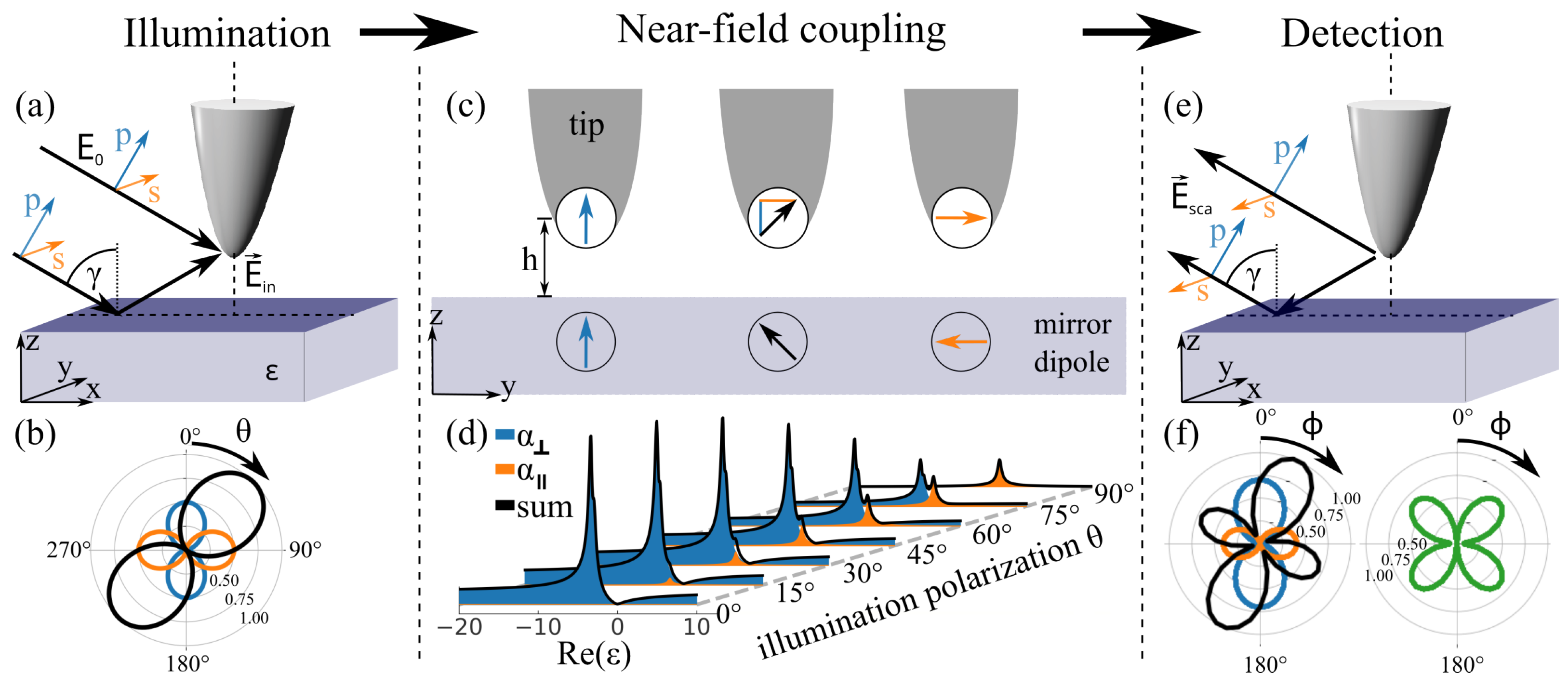
Figure 1. (a) Light polarization geometry of a standard s-SNOM tip under illumination. (b) Linear illumination polarization state with polarization angle $\theta$ = 45${}^{°}$, separated into individual ‘p’ (blue) and ’s’ (orange) polarized contributions, according to the Jones matrix formalism [33]. (c) Interaction between the tip dipole and image dipole according to the point-dipole model for ’p’, ${45}^{°}$, and ’s’ polarized excitation, respectively. (d) Polarizability tensor elements as a function of $\theta$ and Re($\epsilon$) (with $Im(\epsilon$) = 0.2, $\gamma$ = 60${}^{°}$) highlighting the in-plane and out-of-plane resonances of the near-field coupling at $Re\left({\epsilon }_{res,\Vert }\right)=-1.72$ and $Re\left({\epsilon }_{res,\perp }\right)=-3.35$, respectively. (e) Backscattering geometry setup. (f) The complex polarization state of the backscattered signal showing the ’p’ (blue), ’s’ (orange), and mixed (green) contributions. Quantifying this distribution is the goal of this paper here.

Figure 1. (a) Light polarization geometry of a standard s-SNOM tip under illumination. (b) Linear illumination polarization state with polarization angle $\theta$ = 45${}^{°}$, separated into individual ‘p’ (blue) and ’s’ (orange) polarized contributions, according to the Jones matrix formalism [33]. (c) Interaction between the tip dipole and image dipole according to the point-dipole model for ’p’, ${45}^{°}$, and ’s’ polarized excitation, respectively. (d) Polarizability tensor elements as a function of $\theta$ and Re($\epsilon$) (with $Im(\epsilon$) = 0.2, $\gamma$ = 60${}^{°}$) highlighting the in-plane and out-of-plane resonances of the near-field coupling at $Re\left({\epsilon }_{res,\Vert }\right)=-1.72$ and $Re\left({\epsilon }_{res,\perp }\right)=-3.35$, respectively. (e) Backscattering geometry setup. (f) The complex polarization state of the backscattered signal showing the ’p’ (blue), ’s’ (orange), and mixed (green) contributions. Quantifying this distribution is the goal of this paper here.

Figure 1a sketches the tip-sample system and illumination geometry as used for the study here, both theoretically and experimentally. The electric field at the position of the tip ${\overrightarrow{E}}_{in}$ is described as:

$${\overrightarrow{E}}_{in}=\left(\begin{array}{c}{E}_x\\ E_y\\ E_z\end{array}\right)=\left(\begin{array}{ccc}1-r_p& 0& 0\\ 0& 1+r_s& 0\\ 0& 0& 1+r_p\end{array}\right)·\left(\begin{array}{c}cos\left(\gamma \right)cos\left(\theta \right)\\ sin\left(\theta \right)\\ sin\left(\gamma \right)cos\left(\theta \right)\end{array}\right)·E_0,$$

(1)

with $E_0$ the electric field amplitude of the incident light, $\theta$ the linear polarization angle of the incident beam ($\theta =0^{°}$ corresponds to p-polarization), $\gamma$ the incident angle relative to the sample normal, and $r_s$ and $r_p$ the polarization-dependent Fresnel reflection coefficients. Note that any excitation polarization (except for strict s-polarization with $\theta ={90}^{°}$) results in both an in- and out-of-plane electric field excitation at the tip-sample junction. Figure 1b illustrates such a state for $\theta ={45}^{°}$ indicating both p-(blue) and s-polarized (orange) components (see also discussion below).

To calculate the near-field interaction of ${\overrightarrow{E}}_{in}$ with an ideal isotropic sample of permittivity $\epsilon$, the point-dipole model is applied [32]. We define the tip polarizability assuming a spherical tip of radius a, as ${\alpha }_{tip}=4\pi a^3$. It follows:

$${\overrightarrow{P}}_{tot}\sim {\widehat{\alpha }}_{tot}{\overrightarrow{E}}_{in}=\left(\begin{array}{ccc}{\alpha }_x(\epsilon ,h)& 0& 0\\ 0& {\alpha }_y(\epsilon ,h)& 0\\ 0& 0& {\alpha }_z(\epsilon ,h)\end{array}\right)·\left(\begin{array}{c}{E}_x\\ E_y\\ E_z\end{array}\right),$$

(2)

with ${\alpha }_i$ the tensor elements of the tip-sample-coupled polarizability tensor ${\widehat{\alpha }}_{tot}$ and h the tip-dipole-to-sample distance. Using Equation (2), we can separate the near-field coupling into perpendicular (left, blue) and parallel (right, orange)-oriented dipole components as depicted in Figure 1c. The corresponding image dipoles hence will be purely perpendicular and parallel-oriented as well. For non-resonant excitation of that spherical tip positioned above an isotropic sample, the different contributions to ${\widehat{\alpha }}_{tot}$ are given as [32]:

$${\alpha }_z(\epsilon ,h)={\alpha }_{\perp }(\epsilon ,h)=\frac{(1+\beta ){\alpha }_{tip}}{1-\frac{\beta {\alpha }_{tip}}{16\pi h^3}},$$

(3)

$${\alpha }_x(\epsilon ,h)={\alpha }_y(\epsilon ,h)={\alpha }_{\Vert }(\epsilon ,h)=\frac{(1-\beta ){\alpha }_{tip}}{1-\frac{\beta {\alpha }_{tip}}{32\pi h^3}},$$

(4)

with $\beta =\frac{\epsilon -1}{\epsilon +1}$ the sample response function, and ${\alpha }_{\perp }$ and ${\alpha }_{\Vert }$ referring to the out-of-plane and in-plane total polarizability components with respect to the sample surface, respectively. The calculation becomes more complex but still achievable when considering polarization angles other than $\theta =0^{°},{90}^{°}$ since the electric field then is interacting with both ${\alpha }_{\perp }$ and ${\alpha }_{\Vert }$ at the same time. Such a scenario is illustrated in Figure 1c, center.

Figure 1d displays the mixing of ${\alpha }_{\perp }$ and ${\alpha }_{\Vert }$, as calculated with the s-SNOM tip being in firm contact to a fictive sample surface, characterized by $Im(\epsilon$) = 0.2 = const. for all wavelengths, and the tip-dipole-to-sample distance being h = 0.785a. The latter accounts for a shift of the effective tip-dipole position towards the sample upon near-field interaction, as well as for an effective tip-radius of a = 600 nm according to literature [28,35]. Overall, the out-of-plane response (${\alpha }_{\perp }$) is clearly stronger than the in-plane response (${\alpha }_{\Vert }$). Nevertheless, for certain incident polarization angles (e.g., $\theta ={75}^{°}$), the out-of-plane and in-plane components may reach values that are on the same order of magnitude. Most importantly, both components show resonance peaks at slightly different $Re\left(\epsilon \right)$; here, $Re\left({\epsilon }_{res,\perp }\right)=-3.35$ and $Re\left({\epsilon }_{res,\Vert }\right)=-1.72$, with their exact positions depending on the tip-sample distance h. Since $\epsilon$ is frequency-dependent, spectrally addressing and separating these peaks into in-plane and out-of-plane sample responses becomes possible.

In order to determine the detectability of the local in-plane signals in the far field, the radiation of the point dipole ${\overrightarrow{E}}_{near}$ is calculated [34] in the backscattering geometry used here (see Figure 1e). Moreover, additional far-field contributions ${\overrightarrow{E}}_{far}$, e.g., due to direct backscattering, need to be considered, which are superposed to the near-field contribution, resulting in the total scattered field ${\overrightarrow{E}}_{sca}$ in Jones vector notation, as:

$${\overrightarrow{E}}_{sca}={\overrightarrow{E}}_{far}+{\overrightarrow{E}}_{near}=\left(\begin{array}{c}{p}_{far}\\ s_{far}\end{array}\right)+\left(\begin{array}{c}{p}_{near}\\ s_{near}\end{array}\right),$$

(5)

with $p_{far}$, $s_{far}$, and $p_{near}$, $s_{near}$ describing the p- and s-polarized far- and near-field components, respectively. Note that in this model, we discuss self-homodyne detection by connecting ${\overrightarrow{E}}_{far}$ to the reflectivity of the sample. Nevertheless, the method is directly applicable to other detection schemes as well by adapting ${\overrightarrow{E}}_{far}$ accordingly.

Investigating the polarization signature of the scattered signal at the detector ultimately requires considering all of the optical elements in the detection path as well. For this purpose, the Jones matrix formalism [33] was applied, representing every element (i.e., mirrors, beam splitters, etc.) in the detection path by a matrix. With that, the polarization signature ${\overrightarrow{E}}_{det}$ after the detection apparatus for the self-homodyne case is described as:

$${\overrightarrow{E}}_{det}={\widehat{M}}_{mylar}·{\widehat{M}}_{mirror}·{\overrightarrow{E}}_{sca}={\overrightarrow{E}}_{far}^{{}^{\prime }}+{\overrightarrow{E}}_{near}^{{}^{\prime }}=\left(\begin{array}{c}{p}_{far}^{{}^{\prime }}\\ s_{far}^{{}^{\prime }}\end{array}\right)+\left(\begin{array}{c}{p}_{near}^{{}^{\prime }}\\ s_{near}^{{}^{\prime }}\end{array}\right),$$

(6)

with ${\widehat{M}}_{mylar}$ [36] and ${\widehat{M}}_{mirror}$ being the Jones matrices for the mylar beam splitter and mirror, respectively (see the experimental setup in Figure 2). ${\overrightarrow{E}}_{far}^{{}^{\prime }}$ and ${\overrightarrow{E}}_{near}^{{}^{\prime }}$ refer to the far- and near-field contributions at the detector. The signal intensity is finally given by:

$$I=\mid {\overrightarrow{E}}_{det}{\mid }^2={\overrightarrow{E}}_{far}^{{}^{\prime }2}+2{\overrightarrow{E}}_{far}^{{}^{\prime }}{\overrightarrow{E}}_{near}^{{}^{\prime }}+{\overrightarrow{E}}_{near}^{{}^{\prime }2}.$$

(7)

In order to extract the near-field contribution, typically higher-harmonic demodulation is applied to the detected signal [32]. Therefore, the tip-sample distance h is modulated at the fundamental cantilever eigenfrequency $\Omega$, resulting in a modulation of the near-field signal at higher harmonics $n\Omega$ due to the strongly non-linear near-field vs. distance dependence [32]. In general $|{\overrightarrow{E}}_{far}^{{}^{\prime }}|\gg |{\overrightarrow{E}}_{near}^{{}^{\prime }}|$, but with increasing n, all far-field terms become negligible [32]. Ultimately, it is the mixed term in Equation (7) that is commonly probed by this technique:

$$I_{n\Omega }\approx 2{\overrightarrow{E}}_{far}^{{}^{\prime }}{\overrightarrow{E}}_{near,n\Omega }^{{}^{\prime }}=2(p_{far}^{{}^{\prime }}{p}_{near,n\Omega }^{{}^{\prime }}+s_{far}^{{}^{\prime }}{s}_{near,n\Omega }^{{}^{\prime }}).$$

(8)

Here, we clearly see that, firstly, p- and s-polarized near-field contributions generally mix with their corresponding far-field component, but secondly, that p-polarization can be clearly separated from s-polarization when using polarizers and analyzers in the overall s-SNOM setup. The experimental confirmation of this finding is discussed below in Section 4.1.

The mixing of the far and near field for any polarization is expected to be more complicated. In order to further disentangle the different vectorial near-field components, an analyzer is placed in front of the detector. The analyzer Jones matrix reads as:

$${\widehat{M}}_{analyzer}=\left(\begin{array}{cc}cos{\left(\varphi \right)}^2& cos\left(\varphi \right)sin\left(\varphi \right)\\ sin\left(\varphi \right)cos\left(\varphi \right)& sin{\left(\varphi \right)}^2\end{array}\right),$$

(9)

with $\varphi$ denoting the analyzer angle with respect to the p-polarization axis. The optical transmission in the detection path then becomes:

$$\begin{array}{cc}\hfill I_{analyzer}& =\mid {\widehat{M}}_{analyzer}·{\overrightarrow{E}}_{det}{\mid }^2\hfill \\ \hfill & =cos{\left(\varphi \right)}^2({p_{far}^{{}^{\prime }}}^2+2p_{far}^{{}^{\prime }}{p}_{near}^{{}^{\prime }}+{p_{near}^{{}^{\prime }}}^2)\hfill \\ \hfill & +sin{\left(\varphi \right)}^2({s_{far}^{{}^{\prime }}}^2+2s_{far}^{{}^{\prime }}{s}_{near}^{{}^{\prime }}+{s_{near}^{{}^{\prime }}}^2)\hfill \\ \hfill & +\underset{=sin\left(2\varphi \right)}{\underbrace{2cos\left(\varphi \right)sin\left(\varphi \right)}}(p_{far}^{{}^{\prime }}{s}_{far}^{{}^{\prime }}+\underline{p_{far}^{{}^{\prime }}{s}_{near}^{{}^{\prime }}}+\underline{p_{near}^{{}^{\prime }}{s}_{far}^{{}^{\prime }}}+p_{near}^{{}^{\prime }}{s}_{near}^{{}^{\prime }}).\hfill \end{array}$$

(10)

Here, the total signal intensity has three terms, with the first two terms describing strict p- and s-polarized states. They represent the linear polarized contributions for the trivial cases of $s_{far}=s_{near}=0$ and $p_{far}=p_{near}=0$, respectively. However, the third term accounts for the mixing of s- and p-polarized components, which intriguingly includes cross-linked terms of far and near field (see underlined terms in Equation (10)). Moreover, this mixed term is no longer linearly polarized but shows a clover-like intensity distribution with orthogonal maxima at ±45${}^{°}$ due to its $2\varphi$ periodicity (see again Equation (10)). Hence, for any incident polarization that is not strictly p- or s-polarized, a mixed polarization state can not be avoided. Extraction of these terms, again, is achieved by higher-harmonic demodulation at $n\Omega$, then reducing Equation (10) to:

$$\begin{array}{cc}\hfill I_{analyzer}& \simeq cos{\left(\varphi \right)}^2·2p_{far}^{{}^{\prime }}{p}_{near,n\Omega }^{{}^{\prime }}\hfill \\ \hfill & +sin{\left(\varphi \right)}^2·2s_{far}^{{}^{\prime }}{s}_{near,n\Omega }^{{}^{\prime }}\hfill \\ \hfill & +sin\left(2\varphi \right)·(p_{far}^{{}^{\prime }}{s}_{near,n\Omega }^{{}^{\prime }}+p_{near,n\Omega }^{{}^{\prime }}{s}_{far}^{{}^{\prime }}).\hfill \end{array}$$

(11)

The three components of Equation (11) are calculated by python-based simulations and are displayed in Figure 1f. Note that Equations (8) and (11) form the basis for the fitting algorithm that we will apply below for data analysis, finally allowing us to extract the sample’s local permittivities.

Figure 2. s-SNOM setup for the polarization-sensitive measurement scheme. The light of a CO₂ laser is reflected by a mylar beamsplitter and focused via a parabolic mirror (PM) onto the SFM. The backscattered light is collected by the same PM, transmitted through the beamsplitter and detected by an MCT detector. Illumination polarization ($\theta$) control is implemented by adding a 180${}^{°}$ phase retardation plate before the beamsplitter, whereas a grid polarizer is included in the detection path to analyze the scattered signal’s polarization ($\varphi$).

Figure 2. s-SNOM setup for the polarization-sensitive measurement scheme. The light of a CO₂ laser is reflected by a mylar beamsplitter and focused via a parabolic mirror (PM) onto the SFM. The backscattered light is collected by the same PM, transmitted through the beamsplitter and detected by an MCT detector. Illumination polarization ($\theta$) control is implemented by adding a 180${}^{°}$ phase retardation plate before the beamsplitter, whereas a grid polarizer is included in the detection path to analyze the scattered signal’s polarization ($\varphi$).

3. Experimental Setup

For polarization analysis of the near-field signatures, a backscattering s-SNOM setup was adapted to include linear polarization control of both illumination and detection light paths, using a fully ${360}^{°}$ rotatable phase retardation plate and a grid polarizer as analyzer, respectively. The setup is shown in Figure 2.

The self-homodyne s-SNOM setup utilizes a p-polarized temperature-tunable CO₂ laser (Access Laser Co., Everett, WA, USA). Polarization control of the illuminating light is implemented by rotating the p-polarized incident state using a ZnSe 180° phase retardation plate (Thorlabs Inc., Bergkirchen, Germany), which is placed in front of the mylar beamsplitter (homebuilt). Note that reflection and transmission at the mylar beamsplitter itself are strongly polarization dependent, which is taken into account via the Jones matrix ${\widehat{M}}_{mylar}$ as discussed above and in [36]. The reflected part of the laser light gets directed towards a parabolic mirror (2${}^{″}$ diameter, 90${}^{°}$-off-axis, 3${}^{″}$ focal length) by a single gold mirror and is then focused onto the SNOM tip of a homebuilt SFM. Any light scattered off the tip-sample junction is then collected in backscattering geometry by the same parabola and directed toward the mylar beamsplitter via the gold mirror. The detection signal passes the mylar beamsplitter and eventually also the analyzer before then being focused onto the MCT detector (Teledyne Judson Technologies, Montgomeryville, PA, USA; Model J15D12) via a second parabolic mirror.

All polarization measurements were performed with the s-SNOM tip kept at a fixed sample position (x,y), hence recording point-spectra. The higher-harmonic demodulation has been realized via a lock-in amplifier (integration time 50 ms), at multiples $n=2$ of the tip oscillation frequency $\Omega \approx$ 160 kHz. In order to investigate the role of polarization in s-SNOM, three configurations/experiments were carried out with our setup, as will be detailed in the chapters to follow:

• Section 4.1 and Figure 3:
  $\theta$ controlled via the phase retardation plate, with no analyzer;
• Section 4.2 and Figure 4:
  $\theta ={45}^{°}$ set via the phase retardation plate; $\varphi$ probed via the analyzer;
• Section 4.2 and Figure 5:
  $\theta$ controlled the via phase retardation plate; $\varphi$ probed via the analyzer.

4. Results

4.1. Impact of Illumination Polarization

As discussed in Section 2, the in-plane near-field response is strongly connected to resonant excitation at certain values of the sample permittivity. The correlation between in- and out-of-plane near-field signals can therefore be directly connected to the sample’s local permittivity. In the following, we thus compare the near-field response of a gold sample at 10.6 µm ($Re\left(\epsilon \right)=-5146.8$ [37]), as a metallic non-resonant reference sample, to 3C-SiC excited resonantly at 10.6 µm ($Re\left(\epsilon \right)=-1.40$ [38]) and 10.7 µm ($Re\left(\epsilon \right)=-1.94$ [38]). Note that here, gold as a spectrally flat, non-resonant sample has been chosen as its metallic character suppresses any in-plane electric field components at its surface, whereas, on the other hand, the undoped, isotropic 3C-SiC shows a phononic-based near-field resonance at CO₂-laser wavelengths that supports local near-field signals at all polarization angles (see Section 2 and Figure 1).

In order to first investigate the role of in-plane excitation experimentally, the illumination polarization is controlled via the 180° phase retardation plate (see Figure 2), whereas detection is realized without using any analyzer. This corresponds to an intensity distribution as mathematically described by Equation (8). Figure 3 shows this intensity distribution for the second-harmonic demodulation, plotted vs. $\theta$. Each data point represents the integrated signal of all polarization components of the scattered signal. The data sets in Figure 3 were then fitted using Equation (8) and normalized individually for better comparison.

Figure 3. Second harmonic demodulated signal for rotating illumination polarization $\theta$ for different materials and illumination wavelengths. Here, ${\theta }_p=0^{°},{180}^{°},{360}^{°}$ and ${\theta }_s={90}^{°},{270}^{°}$. Data are fitted using Equation (8) (black line), and p- and s-polarization-dominated contributions are shaded in blue and orange, respectively. (a) The gold sample illuminated with $\lambda =10.6\mathsf{\mu }$m shows no response for s-polarized excitation. (b) 3C-SiC illuminated at $\lambda =10.7\mathsf{\mu }$m shows a weak response to s-polarized illumination only, whereas (c) an increased s-polarized response is observed when the illumination wavelength hits the sample’s in-plane phonon resonance at $\lambda =10.6\mathsf{\mu }$m. All three datasets are fitted for their local sample permittivity (see Table 1).

Figure 3. Second harmonic demodulated signal for rotating illumination polarization $\theta$ for different materials and illumination wavelengths. Here, ${\theta }_p=0^{°},{180}^{°},{360}^{°}$ and ${\theta }_s={90}^{°},{270}^{°}$. Data are fitted using Equation (8) (black line), and p- and s-polarization-dominated contributions are shaded in blue and orange, respectively. (a) The gold sample illuminated with $\lambda =10.6\mathsf{\mu }$m shows no response for s-polarized excitation. (b) 3C-SiC illuminated at $\lambda =10.7\mathsf{\mu }$m shows a weak response to s-polarized illumination only, whereas (c) an increased s-polarized response is observed when the illumination wavelength hits the sample’s in-plane phonon resonance at $\lambda =10.6\mathsf{\mu }$m. All three datasets are fitted for their local sample permittivity (see Table 1).

For the non-resonant excitation of gold (Figure 3a), a strong signal excited by p-polarized illumination (${\theta }_p$ = 0${}^{°}$, 180${}^{°}$, and 360${}^{°}$) is observed together with an expected drop in intensity when rotating towards s-polarization (for ${\theta }_s$ = 90${}^{°}$ and 270${}^{°}$) (see Figure 3a). At ${\theta }_s$, the signal reduces to $I_s=0$, matching well to the dipole-model-based simulations. This behavior can be understood as a consequence of the boundary conditions of the dipole field at the metallic sample surface, where only electric field components perpendicular to the sample surface are allowed, hence suppressing any in-plane contributions.

This condition changes for the resonantly excited 3C-SiC sample, for which in-plane field components at the boundary are supported. Consequently, when exciting 3C-SiC at 10.7 µm (Figure 3b), for s-polarized excitation, a non-zero near-field signal is observed, matching the theoretical prediction. Furthermore, when tuning the wavelength closer to the spectral resonances at 10.6 µm, the signal for s-polarized excitation increases (see Figure 3c) to about 25% of the intensity at p-polarized excitation. This clearly underlines that in-plane near-field excitation indeed is possible, leading to a quite strong and measurable s-SNOM signal. Furthermore, the intensity of the in-plane signal correlates with the resonance as predicted by the point-dipole model.

In order to fit the data, Equation (8) was used, leading to a qualitatively correct result for all three plots in Figure 3. As result of fitting, the sample permittivities could be extracted (see Table 1), illustrating two findings: firstly, the highly non-resonant nature of gold at 10.6 µm can be reproduced by the fit. Secondly, the comparably small difference in sample permittivity for resonant excitation could be resolved successfully for 3C-SiC at 10.6 µm and 10.7 µm, respectively. The deviation between the values determined by us and the literature values is likely caused by inaccurate fitting for a single polarization line. In particular, as detailed in Section 2, the near-field interaction depends on, e.g., tip radius, modulation amplitude, and tip-sample distance in addition to sample permittivity. These important system parameters are not fitted reliably by the single-line measurement and need to be taken into account. To increase the accuracy further and thereby enable a more detailed polarization examination, in the following an analyzer will be added to the detection path.

Table 1. $Re\left(\epsilon \right)$ for Au and 3C-SiC as extracted through fitting the experimental results shown in Figure 3 by applying Equation (8).

Sample	Re($\mathit{\epsilon }$); Our Result	Re($\mathit{\epsilon }$); Literature
Au @ 10.6 µm	−6521.02	−5146.8 [37]
3C-SiC @ 10.7 µm	−18.23 ± 1.55	−1.94 [38]
3C-SiC @ 10.6 µm	−4.27 ± 0.53	−1.40 [38]

Table 1. $Re\left(\epsilon \right)$ for Au and 3C-SiC as extracted through fitting the experimental results shown in Figure 3 by applying Equation (8).

Sample	Re($\mathit{\epsilon }$); Our Result	Re($\mathit{\epsilon }$); Literature
Au @ 10.6 µm	−6521.02	−5146.8 [37]
3C-SiC @ 10.7 µm	−18.23 ± 1.55	−1.94 [38]
3C-SiC @ 10.6 µm	−4.27 ± 0.53	−1.40 [38]

4.2. Analyzing the Near-Field Polarization

In addition to measuring the integrated signal at a defined illumination polarization, we furthermore investigate the nature of complex far- and near-field mixing by analyzing the polarization distribution of the scattered light. Therefore, the different contributions in the backscattered signal are separated by an analyzer at the angle $\varphi$ with respect to p-polarization.

As an exemplary measurement, we excite 3C-SiC resonantly at 10.6 µm with ($\theta ={45}^{°}$)-polarized incident light (Figure 4). The overall signal (see Figure 4a) shows a non-trivial polarization state with four lobes, the maxima of which are 90${}^{°}$ apart. The stronger lobe is oriented along the 25${}^{°}$ axis, leaving an offset of ∼${20}^{°}$ with respect to the illumination polarization. In order to extract the underlying polarization contributions, the lobe is fitted using Equation (11), resulting in an excellent match. Moreover, the fit allows for a separation of the individual terms and hence for the extraction of individual signal contributions. The corresponding separated p-polarized, s-polarized, and mixed terms are shown in Figure 4b–d, respectively, with the overall signal in grey for comparison. Comparing p- and s-polarized contributions, the out-of-plane field enhancement of the former is apparent, yielding a five times higher signal intensity. However, this comparably small s-polarized contribution causes a significant rotation of the overall light distribution due to the mixed term. Referring to Equation (11), the origin of this enhancement is found in the mixing of the p-polarized far-field term with the s-polarized near-field term and vice versa, resulting in the clover-like polarization response as displayed in Figure 4d.

Figure 4. Polarization distribution of the near-field signal for a 3C-SiC sample measured as a function of analyzer rotation $\varphi$ ($\lambda$ = 10.6 µm, $\theta$ = 45${}^{°}$). (a) Overall distribution and fit; (b) p-polarized (blue), (c) s-polarized (orange), and (d) mixed contributions (green), calculated and extracted from the fit showing a strong coupling even for small s-polarized contributions due to component mixing (see Equation (11)). For comparison, the fitted overall distribution from (a) is reproduced in gray in (b–d).

Figure 4. Polarization distribution of the near-field signal for a 3C-SiC sample measured as a function of analyzer rotation $\varphi$ ($\lambda$ = 10.6 µm, $\theta$ = 45${}^{°}$). (a) Overall distribution and fit; (b) p-polarized (blue), (c) s-polarized (orange), and (d) mixed contributions (green), calculated and extracted from the fit showing a strong coupling even for small s-polarized contributions due to component mixing (see Equation (11)). For comparison, the fitted overall distribution from (a) is reproduced in gray in (b–d).

In order to explore the origin of the complex polarization mixing, we extend our measurements to a full set of incident and scattered polarizations as displayed in Figure 5. Here, the intensity distribution in each horizontal line represents one full rotation of the analyzer angle ($\varphi$), while the vertical axis corresponds to varying incident polarization angles $\theta$. We refer to the resulting 2D plot as a “polarization point spectrum”.

Figure 5. Normalized polarization point spectrum of 3C-SiC at 10.6 µm. (a) The polarization point spectrum was measured by rotating the analyzer ($\varphi$) by 360${}^{°}$ for each illumination polarization angle ($\theta$). (b) The 2D fit of the polarization point spectra matches well with the experimental results and is used to extract the local sample permittivity (see Table 2).

Figure 5. Normalized polarization point spectrum of 3C-SiC at 10.6 µm. (a) The polarization point spectrum was measured by rotating the analyzer ($\varphi$) by 360${}^{°}$ for each illumination polarization angle ($\theta$). (b) The 2D fit of the polarization point spectra matches well with the experimental results and is used to extract the local sample permittivity (see Table 2).

Due to the symmetry of the underlying polarization, the polarization point spectrum (see Figure 5) has a twofold symmetry (and hence self-reproduces every 180${}^{°}$). Furthermore, the strongest signal is observed for p-polarized illumination, for $\theta =0^{°},{180}^{°},{360}^{°}$ and p-polarized detection at $\varphi =0^{°},{180}^{°},{360}^{°}$, as expected when comparing it to the integrated intensity distribution in Figure 3c. Moreover, side maxima are observed for s-polarized analyzer angles at $\varphi \approx {90}^{°}$.

In order to fit the data, Equation (11) is used, in analogy to the fit for Figure 4a as described above. The function was modified, however, to fit the entire polarization point spectrum recursively. Qualitatively, the resulting fit resembles the experimental data very accurately, including both the global maxima at $\theta$, $\varphi =0^{°},{180}^{°}$, and ${360}^{°}$, as well as the corresponding side maxima. The latter resembles the creation of side lobes as connected to the mixing of far- and near-field components with different polarization states (see Equation (11)). Quantitatively, the recursive fit enables the determination of the sample’s permittivities at two different wavelengths as summarized in Table 2, which are close but not perfectly matching the values found in literature. Deviations might be related to the spherical tip shape assumed here as part of the point-dipole model. Especially, inaccuracies regarding the out-of-plane electric field enhancement are reported to impact the quality of the model [27]. The fit might be improved further by implementing more realistic tip shapes [23]. However, compared to the investigation of incident polarization only as summarized in Table 1, the advanced polarization-point-spectrum fit improved the obtained Re($\epsilon$) values significantly, demonstrating the relevance of a complete mapping of near-field signal polarization.

Table 2. Re($\epsilon$) for 3C-SiC evaluated at different wavelengths, resulting from fitting the polarization point spectra using Equation (10).

Wavelength	Re($\mathit{\epsilon }$); Our Results	Re($\mathit{\epsilon }$); Literature
10.6 µm	−2.57 ± 0.54	−1.40 [38]
10.7 µm	−6.37 ± 0.73	−1.94 [38]

Table 2. Re($\epsilon$) for 3C-SiC evaluated at different wavelengths, resulting from fitting the polarization point spectra using Equation (10).

Wavelength	Re($\mathit{\epsilon }$); Our Results	Re($\mathit{\epsilon }$); Literature
10.6 µm	−2.57 ± 0.54	−1.40 [38]
10.7 µm	−6.37 ± 0.73	−1.94 [38]

Overall, the successful extraction of local permittivity data from polarization point spectra demonstrates the potential of polarization-controlled s-SNOM for local material characterization.

5. Conclusions

In summary, we demonstrated that resonant sample excitation in s-SNOM results in significant in-plane contributions that can be addressed individually by adjusting the illumination polarization angle accordingly. The in-plane response is strongly connected to the sample permittivity, as demonstrated for resonantly and non-resonantly excited samples. Moreover, the mixing between s- and p-polarized far- and near-field components was demonstrated to lead to a rotation in the scattered polarization, even for small s-polarized contributions. Finally, full polarization analysis enables the extraction of the local permittivity data via a recursive fit algorithm that matches well to the values reported in literature.

More generally, by demonstrating the existence and reading of in-plane near-field components, this fundamental work forms an important pillar for future polarization-sensitive s-SNOM application scenarios, such as nanoellipsometry, e.g., by also introducing circularly-polarized field excitation. Particularly, we envision the application towards in-plane sensitive and anisotropic samples such as 2D van-der-Waals and topological materials.

References

- Rao, V.J.; Matthiesen, M.; Goetz, K.P.; Huck, C.; Yim, C.; Siris, R.; Han, J.; Hahn, S.; Bunz, U.H.F.; Dreuw, A.; et al. AFM-IR and IR-SNOM for the Characterization of Small Molecule Organic Semiconductors. J. Phys. Chem. C 2020, 124, 5331–5344. [Google Scholar] [CrossRef]
- Tesema, T.E.; Mcfarland-Porter, R.; Zerai, E.; Grey, J.; Habteyes, T.G. Hierarchical Self-Assembly and Chemical Imaging of Nanoscale Domains in Polymer Blend Thin Films. J. Phys. Chem. C 2022, 126, 7764–7772. [Google Scholar] [CrossRef]
- Dai, S.; Zhang, J.; Ma, Q.; Kittiwatanakul, S.; Mcleod, A.; Chen, X.; Gilbert Corder, S.; Watanabe, K.; Taniguchi, T.; Lu, J.; et al. Phase-Change Hyperbolic Heterostructures for Nanopolaritonics: A Case Study of hBN/VO2. Adv. Mater. 2019, 31, 1900251. [Google Scholar] [CrossRef]
- Ritchie, E.T.; Casper, C.B.; Lee, T.A.; Atkin, J.M. Quantitative Local Conductivity Imaging of Semiconductors Using Near-Field Optical Microscopy. J. Phys. Chem. C 2022, 126, 4515–4521. [Google Scholar] [CrossRef]
- Rygula, A.; Oleszkiewicz, T.; Grzebelus, E.; Pacia, M.Z.; Baranska, M.; Baranski, R. Raman, AFM and SNOM high resolution imaging of carotene crystals in a model carrot cell system. Spectrochim. Acta Part A Mol. Biomol. Spectrosc. 2018, 197, 47–55. [Google Scholar] [CrossRef]
- Zenhausern, F.; Martin, Y.; Wickramasinghe, H.K. Scanning interferometric apertureless microscopy: Optical imaging at 10 angstrom resolution. Science 1995, 269, 1083–1085. [Google Scholar] [CrossRef]
- Knoll, B.; Keilmann, F. Near-field probing of vibrational absorption for chemical microscopy. Nature 1999, 399, 134–137. [Google Scholar] [CrossRef]
- Hillenbrand, R.; Knoll, B.; Keilmann, F. Pure optical contrast in scattering-type scanning near-field microscopy. J. Microsc. 2001, 202, 77–83. [Google Scholar] [CrossRef]
- Taubner, T.; Hillenbrand, R.; Keilmann, F. Performance of visible and mid-infrared scattering-type near-field optical microscopes. J. Microsc. 2003, 210, 311–314. [Google Scholar] [CrossRef] [PubMed]
- Huber, A.J.; Keilmann, F.; Wittborn, J.; Aizpurua, J.; Hillenbrand, R. Terahertz near-field nanoscopy of mobile carriers in single semiconductor nanodevices. Nano Lett. 2008, 8, 3766–3770. [Google Scholar] [CrossRef]
- Kuschewski, F.; Von Ribbeck, H.G.; Döring, J.; Winnerl, S.; Eng, L.M.; Kehr, S.C. Narrow-band near-field nanoscopy in the spectral range from 1.3 to 8.5 THz. Appl. Phys. Lett. 2016, 108, 113102. [Google Scholar] [CrossRef]
- de Oliveira, T.V.; Nörenberg, T.; Álvarez-Pérez, G.; Wehmeier, L.; Taboada-Gutiérrez, J.; Obst, M.; Hempel, F.; Lee, E.J.; Klopf, J.M.; Errea, I.; et al. Nanoscale-Confined Terahertz Polaritons in a van der Waals Crystal. Adv. Mater. 2021, 33, 2005777. [Google Scholar] [CrossRef]
- Huber, A.; Ocelic, N.; Taubner, T.; Hillenbrand, R. Nanoscale Resolved Infrared Probing of Crystal Structure and of Plasmon-Phonon Coupling. Nano Lett. 2006, 6, 774–778. [Google Scholar] [CrossRef]
- Cui, T.; Sun, L.; Bai, B.; Sun, H.B. Probing and Imaging Photonic Spin-Orbit Interactions in Nanostructures. Laser Photonics Rev. 2021, 15, 2100011. [Google Scholar] [CrossRef]
- Kehr, S.C.; Cebula, M.; Mieth, O.; Härtling, T.; Seidel, J.; Grafström, S.; Eng, L.M.; Winnerl, S.; Stehr, D.; Helm, M. Anisotropy contrast in phonon-enhanced apertureless near-field microscopy using a free-electron laser. Phys. Rev. Lett. 2008, 100, 256403. [Google Scholar] [CrossRef] [PubMed]
- Govyadinov, A.A.; Mastel, S.; Golmar, F.; Chuvilin, A.; Carney, P.S.; Hillenbrand, R. Recovery of permittivity and depth from near-field data as a step toward infrared nanotomography. ACS Nano 2014, 8, 6911–6921. [Google Scholar] [CrossRef] [PubMed]
- Lee, K.G.; Kihm, H.W.; Kihm, J.E.; Choi, W.J.; Kim, H.; Ropers, C.; Park, D.J.; Yoon, Y.C.; Choi, S.B.; Woo, D.H.; et al. Vector field microscopic imaging of light. Nat. Photon. 2007, 1, 53–56. [Google Scholar] [CrossRef]
- Liu, Z.; Ng, B.P.; Zhang, Y.; Soh, Y.C.; Kok, S.W. Near-field ellipsometry for thin film characterization. Opt. Express 2010, 18, 3298–3310. [Google Scholar] [CrossRef]
- Liu, Z.; Zhang, Y.; Kok, S.W.; Ng, B.P.; Soh, Y.C. Reflection-based near-field ellipsometry for thin film characterization. Ultramicroscopy 2013, 124, 26–34. [Google Scholar] [CrossRef]
- Esslinger, M.; Dorfmüller, J.; Khunsin, W.; Vogelgesang, R.; Kern, K. Background-free imaging of plasmonic structures with cross-polarized apertureless scanning near-field optical microscopy. Rev. Sci. Instrum 2012, 83, 033704. [Google Scholar] [CrossRef] [PubMed]
- Mrkyvkova, N.; Cernescu, A.; Futera, Z.; Nebojsa, A.; Dubroka, A.; Sojkova, M.; Hulman, M.; Majkova, E.; Jergel, M.; Siffalovic, P.; et al. Nanoimaging of Orientational Defects in Semiconducting Organic Films. J. Phys. Chem. C 2021, 125, 42. [Google Scholar] [CrossRef]
- Schneider, S.; Seidel, J.; Grafström, S.; Eng, L.M.; Winnerl, S.; Stehr, D.; Helm, M. Impact of optical in-plane anisotropy on near-field phonon polariton spectroscopy. Appl. Phys. Lett. 2007, 90, 143101. [Google Scholar] [CrossRef]
- McArdle, P.; Lahneman, D.J.; Biswas, A.; Keilmann, F.; Qazilbash, M.M. Near-field infrared nanospectroscopy of surface phonon-polariton resonances. Phys. Rev. Research 2020, 2, 023272. [Google Scholar] [CrossRef]
- Richard, R.; Xinzhong, C.; Mengkun, L. High-efficiency scattering probe design for s-polarized near-field microscopy. Appl. Phys. Express 2021, 14, 022002. [Google Scholar] [CrossRef]
- Park, K.D.; Raschke, M.B. Polarization Control with Plasmonic Antenna Tips: A Universal Approach to Optical Nanocrystallography and Vector-Field Imaging. Nano Lett. 2018, 18, 2912–2917. [Google Scholar] [CrossRef] [PubMed]
- Yao, Z.; Chen, X.; Wehmeier, L.; Xu, S.; Shao, Y.; Zeng, Z.; Liu, F.; Mcleod, A.S.; Gilbert Corder, S.N.; Tsuneto, M.; et al. Probing subwavelength in-plane anisotropy with antenna-assisted infrared nano-spectroscopy. Nat. Commun. 2021, 12, 2649. [Google Scholar] [CrossRef] [PubMed]
- Aminpour, H.; Eng, L.M.; Kehr, S.C. Spatially confined vector fields at material-induced resonances in near-field-coupled systems. Opt. Express 2020, 28, 32316. [Google Scholar] [CrossRef]
- Wehmeier, L.; Lang, D.; Liu, Y.; Zhang, X.; Winnerl, S.; Eng, L.M.; Kehr, S.C. Polarization-dependent near-field phonon nanoscopy of oxides: SrTiO3, LiNbO3, and PbZr0.2Ti0.8O3. Phys. Rev. B 2019, 100, 47–52. [Google Scholar] [CrossRef]
- Huber, A.J.; Ziegler, A.; Köck, T.; Hillenbrand, R. Infrared nanoscopy of strained semiconductors. Nat. Nanotechnol. 2009, 4, 153–157. [Google Scholar] [CrossRef]
- Wehmeier, L.; Nörenberg, T.; De Oliveira, T.V.; Klopf, J.M.; Yang, S.Y.; Martin, L.W.; Ramesh, R.; Eng, L.M.; Kehr, S.C. Phonon-induced near-field resonances in multiferroic BiFeO3 thin films at infrared and THz wavelengths. Appl. Phys. Lett. 2020, 116. [Google Scholar] [CrossRef]
- Döring, J.; Lang, D.; Wehmeier, L.; Kuschewski, F.; Nörenberg, T.; Kehr, S.C.; Eng, L.M. Low-temperature nanospectroscopy of the structural ferroelectric phases in single-crystalline barium titanate. Nanoscale 2018, 10, 18074–18079. [Google Scholar] [CrossRef] [PubMed]
- Knoll, B.; Keilmann, F. Enhanced dielectric contrast in scattering-type scanning near-field optical microscopy. Opt. Commun. 2000, 182, 321–328. [Google Scholar] [CrossRef]
- Jones, R.C. A New Calculus for the Treatment of Optical SystemsI Description and Discussion of the Calculus. J. Opt. Soc. Am. 1941, 31, 488. [Google Scholar] [CrossRef]
- Lukosz, W. Light emission by magnetic and electric dipoles close to a plane dielectric interface. III. Radiation patterns of dipoles with arbitrary orientation. JOSA 1979, 69, 1495–1503. [Google Scholar] [CrossRef]
- Renger, J.; Grafström, S.; Eng, L.M.; Hillenbrand, R. Resonant light scattering by near-field-induced phonon polaritons. Phys. Rev. B 2005, 71, 075410. [Google Scholar] [CrossRef]
- Fymat, A.L. Jones’s Matrix Representation of Optical Instruments I: Beam Splitters. Appl. Opt. 1971, 10, 2499. [Google Scholar] [CrossRef] [PubMed]
- Weaver, J.H.; Babar, S. Optical constants of Cu, Ag, and Au revisited. Appl. Opt. 2015, 54, 477–481. [Google Scholar] [CrossRef]
- Mutschke, H.; Andersen, A.C.; Clément, D.; Henning, T.; Peiter, G. Infrared properties of SiC particles. Astron. Astrophys. 1999, 345, 187–202. [Google Scholar] [CrossRef]
Disclaimer/Publisher’s Note: The statements, opinions and data contained in all publications are solely those of the individual author(s) and contributor(s) and not of MDPI and/or the editor(s). MDPI and/or the editor(s) disclaim responsibility for any injury to people or property resulting from any ideas, methods, instructions or products referred to in the content. |
© 2023 by the authors. Licensee MDPI, Basel, Switzerland. This article is an open access article distributed under the terms and conditions of the Creative Commons Attribution (CC BY) license (https://creativecommons.org/licenses/by/4.0/).
Share and Cite
MDPI and ACS Style
Kaps, F.G.; Kehr, S.C.; Eng, L.M. Polarization Sensitivity in Scattering-Type Scanning Near-Field Optical Microscopy—Towards Nanoellipsometry. Appl. Sci. 2023, 13, 10429. https://0-doi-org.brum.beds.ac.uk/10.3390/app131810429
AMA Style
Kaps FG, Kehr SC, Eng LM. Polarization Sensitivity in Scattering-Type Scanning Near-Field Optical Microscopy—Towards Nanoellipsometry. Applied Sciences. 2023; 13(18):10429. https://0-doi-org.brum.beds.ac.uk/10.3390/app131810429
Chicago/Turabian StyleKaps, Felix G., Susanne C. Kehr, and Lukas M. Eng. 2023. "Polarization Sensitivity in Scattering-Type Scanning Near-Field Optical Microscopy—Towards Nanoellipsometry" Applied Sciences 13, no. 18: 10429. https://0-doi-org.brum.beds.ac.uk/10.3390/app131810429
Note that from the first issue of 2016, this journal uses article numbers instead of page numbers. See further details here.