
Georeferenced Analysis of Urban Nightlife and Noise Based on Mobile Phone Data
by
 , , and
Luís B. Elvas
1,2,3 ,
,
Miguel Nunes
1,
Joao C. Ferreira
1,2,3 ,
,
Bruno Francisco
1 and
Jose A. Afonso
4,* 1
Instituto Universitário de Lisboa (ISCTE-IUL), ISTAR, 1649-026 Lisboa, Portugal
2
Inov Inesc Inovação—Instituto de Novas Tecnologias, 1000-029 Lisbon, Portugal
3
Department of Logistics, Molde University College, 6410 Molde, Norway
4
CMEMS–UMinho and LABBELS–Associate Laboratory, University of Minho, 4800-058 Guimarães, Portugal
*
Author to whom correspondence should be addressed.
Appl. Sci. 2024, 14(1), 362; https://0-doi-org.brum.beds.ac.uk/10.3390/app14010362
Submission received: 25 October 2023
/
Revised: 27 December 2023
/
Accepted: 28 December 2023
/
Published: 30 December 2023
(This article belongs to the Special Issue Applications of Machine Learning in National Territory Spatial Planning)
Abstract
:Urban environments are characterized by a complex soundscape that varies across different periods and geographical zones. This paper presents a novel approach for analyzing nocturnal urban noise patterns and identifying distinct zones using mobile phone data. Traditional noise-monitoring methods often require specialized equipment and are limited in scope. Our methodology involves gathering audio recordings from city sensors and localization data from mobile phones placed in urban areas over extended periods with a focus on nighttime, when noise profiles shift significantly. By leveraging machine learning techniques, the developed system processes the audio data to extract noise features indicative of different sound sources and intensities. These features are correlated with geographic location data to create comprehensive city noise maps during nighttime hours. Furthermore, this work employs clustering algorithms to identify distinct noise zones within the urban landscape, characterized by their unique noise signatures, reflecting the mix of anthropogenic and environmental noise sources. Our results demonstrate the effectiveness of using mobile phone data for nocturnal noise analysis and zone identification. The derived noise maps and zones identification provide insights into noise pollution patterns and offer valuable information for policymakers, urban planners, and public health officials to make informed decisions about noise mitigation efforts and urban development.
1. Introduction
Ongoing urbanization trends have led to the rapid growth of cities, bringing numerous benefits but also introducing challenges, such as noise pollution [1]. This is a significant environmental concern, affecting the health and well-being of city residents [2]. Urban areas are characterized by diverse noise sources, including transportation, industrial activities, construction, and social events. The acoustic environment of a city is highly dynamic, with noise patterns changing across different times and locations [3]. Therefore, understanding and effectively managing urban noise pollution requires innovative approaches that capture the complexity of these patterns [4], such as utilizing machine learning techniques and wireless acoustic sensor networks, as proposed in [5].
The motivation behind this work stems from the need to develop comprehensive and adaptable strategies for assessing and managing noise pollution in cities. Traditional methods of noise monitoring often involve stationary noise sensors placed in specific locations, which may fail to capture the full scope of noise variability across a city. Furthermore, these methods can be costly to deploy and maintain.
The trajectory from noise mapping to action plans and eventual mitigation measures represents a crucial avenue in environmental acoustics, particularly in the context of the evolving landscape of smart and sustainable cities. A paradigm shift has been observed, especially in noise mapping, where innovative solutions are emerging, such as real-time evaluation, enhanced monitoring stations with stringent control measures, and the integration of artificial intelligence applications. Noteworthy advancements include mitigations facilitated by electric vehicles, the integration of low-noise pavements, refined input methodologies, and their real-world contextual evaluations [4,6,7,8,9].
Recent literature underscores the multifaceted developments in wireless acoustic sensor networks for environmental noise monitoring within smart cities [7]. The incorporation of machine learning methods and camera images in intelligent transportation systems (ITS) is contributing to optimized noise maps and action plans [6]. Meanwhile, the integration of the Internet of Things (IoT) for noise mapping in smart cities is a focal point, outlining the state of the art and future directions [7]. Acoustic beamforming algorithms are making strides, with applications in environmental noise [10,11]. Additionally, researchers are defining key performance indicators for noise monitoring networks [12] and utilizing statistical pass-by methods for unattended road traffic noise measurement [13].
In the realm of electric vehicles, there is a dedicated focus on predicting noise emissions, with advancements in models and coefficients [14,15]. Artificial neural networks are employed for predicting annoyance evaluations of electric vehicle noise [16], and machine learning techniques are leveraged for real-time air quality and environmental noise detection [17]. Ensemble models based on artificial intelligence find applications in predicting vehicular traffic noise [18], and deep learning and gradient boosting are making strides in urban environmental noise monitoring in smart cities [19]. The comprehensive landscape presented in these studies underscores the dynamic and interdisciplinary nature of noise research in smart cities.
On the other hand, mobile phones, being an integral part of modern urban life, offer a ubiquitous, unobtrusive and cost-effective means to collect large volumes of data from diverse areas within a city. By harnessing the capabilities of mobile phones, it is possible to obtain insights into the temporal and spatial dynamics of urban noise pollution that were previously challenging to achieve [20].
Integrating mobile phone data into noise analysis holds the promise of revolutionizing how noise pollution in urban environments is understood, monitored, and addressed. By utilizing this approach, there is a move towards more data-driven, adaptable, and efficient noise management practices, ultimately creating healthier and more livable cities for everyone [21].
A combination of noise sensors scattered around a city and mobility data captured by mobile operators represents a comprehensive urban data solution that can provide valuable insights into the dynamics of urban life. Noise sensors are strategically placed throughout the city, typically in areas prone to noise pollution, near transportation hubs, commercial districts, residential neighborhoods, and public spaces. These sensors are equipped with microphones and data collection capabilities. In the context of the data collection process, these noise sensors continuously monitor and record environmental noise levels in real time, capturing information such as decibel levels, frequency spectra, and the time of day when noise events occur. For data transmission, these noise sensors are usually connected to a central data collection device via wired or wireless connections [22]. The collected noise data are then transmitted to a central server through the Internet for further processing and analysis.
The combination of noise sensors and mobile operator mobility data offers a holistic view of urban life, allowing city planners and authorities to make informed decisions, improve services, and enhance the overall well-being of residents while addressing environmental concerns. Data privacy and security are paramount, and are achieved in the context of this work because information was provided not for a specific place, but for the street [23].
This paper’s main contribution is describing and demonstrating a novel approach for analyzing nocturnal urban noise patterns and identifying distinct noise zones using mobile phone data and stationary noise sensors. By leveraging machine learning (ML) and clustering techniques, it is possible to process the collected audio recordings and location data to create detailed noise maps and categorize zones based on their noise signatures. The resulting insights can inform urban planning decisions, guide noise mitigation strategies, and improve city residents’ quality of life. Based on our work, municipalities may understand nightlife patterns better, and decisions can be made based on these data.
The rest of this paper is organized as follows. Section 2 presents a literature review highlighting the work related to the subject of this paper. Section 3 describes the datasets used in this work and their pre-processing, while Section 4 describes the process of identifying the nightlife areas and the corresponding results. Finally, Section 5 presents the conclusions and suggestions for future work.
2. Related Work
The literature surrounding the analysis of nocturnal urban noise and the identification of noise zones using mobile phone data in a city reveals a growing interest in leveraging technological advancements for a more accurate and comprehensive understanding of urban soundscapes. This section reviews key studies and approaches that contribute to the foundation of the proposed research.
The methodology employed in this literature review is based on PRISMA (Preferred Reporting Items for Systematic Reviews and Meta-Analyses) [24], which is a widely recognized and extensively used framework for conducting and reporting systematic reviews and meta-analyses in healthcare, social sciences, and other disciplines.
2.1. Search Strategy and Inclusion Criteria
This literature review was conducted in September 2023, and the applied filters were designed to consider only research articles and reviews published in English-language journals from the past five years. The databases selected for searching publications were the Scopus database and the Web of Science Core Collection.
To restrict our search to relevant results, the constructed query included the concepts of “machine learning”, “data analytics”, “artificial intelligence”, or “pattern recognition” in the context of “smart cities”, “mobile data”, or “mobile operator data”, targeting the works related to “nightlife”, “noise detection”, “noise pollution”, “noise monitoring”, “noise zoning”, or “soundscape analysis”.
2.2. Search Results and Analysis
The constructed query returned 37 publications from both databases. Following the download of these publications, the application of the PRISMA methodology began with the elimination of duplicates, which resulted in 23 publications that warranted detailed reading. Figure 1 illustrates the results of the application of the PRISMA workflow to this literature review.
In this literature review, our primary objective was to investigate the existing research works related to the analysis and mapping of nightlife noise, using ML techniques, in order to comprehend potential patterns. Table 1 summarizes the topics identified in the literature review ordered by the number of documents. As is evident, machine learning, the Internet of Things (IoT), and deep learning play a significant role in noise monitoring and the study and comprehension of noise pollution. Additionally, some studies also address the topics of smart traffic and noise prediction.
In ref. [25], Albaji et al., investigate the use of ML models to classify environmental sounds that are considered noise pollution in smart cities. Different types of noise were collected in sixteen cities in Malaysia. The best ML sound classification model achieved results with an accuracy score exceeding 0.95.
In ref. [26], Toutouh et al., use an IoT system to monitor noise at a university campus in Spain. Using ML techniques, the authors found that most university community members move through the campus at similar hours, causing congestion and acoustic pollution above regulation limits. In [27], Bhoi et al. present a sismilar study, performed in India, aimed to understand the levels of noise pollution during relevant events. The authors proposed an ML model to predict noise pollution, achieving an accuracy higher than 90%.
Middya et al. [28] use IoT and ML to better understand and combat noise pollution. Their framework can successfully detect noise levels above tolerable limits. Monti et al. [33] also combine IoT and ML to better inspect and monitor urban noise. In ref. [30], Hernandez-Jayo et al., combine ML techniques with a geo-sensing application to help decision makers have as much information as possible. The main function of the framework is to provide real-time information on the acoustic impact on the city and they also provide an ML module capable of predicting the nature of the noise with an acceptable percentage of accuracy.
Zamora et al. [32] present a robust environmental noise monitoring system that utilizes smartphones and cloud services for high spatial granularity. The architecture efficiently captures noise pollution data through mobile sensors and Firebase technology, achieving substantial energy and computing savings of approximately 60%. While slight measurement variations were noted among different smartphones, they were generally not significant.
Liu et al. [8] discuss the use of IoT solutions to help monitor and map noise in smart cities. Cost, accuracy, scalability, reliability and capability are discussed in order to find the best solution. In ref. [34], Middya et al. also use IoT technologies, combined with spatial interpolation techniques and real-world participatory sensing-based datasets collected by participants over a period of one year, to help monitor noise pollution.
The authors in refs. [19,35,37] focus on using deep learning techniques to help monitor and classify noise, detect noise level anomalies and even predict noise pollution for various periods, from 1 to 60 min.
In ref. [38], Zhang et al. use deep learning to predict traffic noise. The authors achieved the best performance with a multivariate bi-directional GRU (Gated Recurrent Unit) model with many-to-many architecture, featuring both high accuracy and computation efficiency.
The works described in refs. [29,31,36,39] are less related to the scope of this paper. In ref. [31], Kaarivuo et al., discuss the utilization of ML techniques to create frameworks for urban soundscape planning and, consequently, to create healthy urban soundscapes; papers [29,39] focus on smart traffic control as a way to reduce noise pollution in cities.
Overall, these works understand the importance of controlling urban noise, which is one of the most serious and underestimated environmental problems. According to Monti et al., noise pollution from traffic and other human activities has a significant negative impact on the health and quality of life of the populations [33].
Compared with the literature, this work employs machine learning approaches to comprehend noise patterns during the nightlife period and provide decision makers with the tools they need to make better and more informed decisions. Our work uses real data and can be replicated in other cities.
3. Data and Methodology
The primary dataset used in this project was initially compiled by the telecommunications company and was provided by the Lisbon City Council. The information in the dataset includes the number of mobile phones that entered, remained, and exited 3743 grid cells in Lisbon, each one measuring 200 by 200 m, from 15 September 2021 to 31 December 2022. The 24 variables of this dataset are shown in Table 2, along with their respective descriptions.
As mentioned before, the available dataset was limited to the telecommunications company’s customers only. Recognizing the need to understand the broader mobile phone usage in the area, the Lisbon City Council took the initiative to process this dataset further, in order to estimate the total number of mobile phones of all telecommunications companies in each grid, including the other two main telecommunications companies operating in the area.
By understanding telecommunications company’s market share, the Lisbon City Council was able to make estimates about the overall mobile phone usage in the area, encompassing all companies. For instance, if a telecommunications company’s market share is known to be a certain percentage, say 30%, of the total telecom market in that area, and the telecommunications company reports a specific number of users, this information can be used to extrapolate or estimate the total number of users across all companies. This method allowed for a more comprehensive understanding of mobile phone usage across all telecommunications operators in the region, despite the lack of direct user data from some companies.
3.1. Data Pre-Processing
The pre-processing of the dataset was straightforward, due to the well-prepared nature of the provided data. During the analysis to identify missing, duplicate, and incorrectly formatted data, it was also discovered that dates without records were absent from the dataset. This pattern was observed across all variables. Additionally, variables D1 and E6 contained NaN (not a number) values. As these two variables were not relevant to our work, they were excluded, resulting in a clean dataset without any NaN values. Nevertheless, in practical terms, there were dates without records that were not included in the dataset, indicating data flaws. In places with missing values, the complete entry was removed, reducing the amount of data by 3%.
3.1.1. Identification of Flaws in the Data
The task of identifying flaws in the provided dataset arose from the need to create time series, which cannot have interruptions. This analysis was conducted in two stages: an initial one, in which flaws in all grids lasting over 24 h were identified; and a more in-depth one, in which all 5-min periods with flaws were identified for each grid individually.
The records were registered in intervals of 5 min, and all the intervals that contained flaws were identified. Total and partial flaws were distinguished, with total flaws corresponding to failures in all grids, and partial flaws corresponding to failures in only some grids.
3.1.2. Imputation of Missing Values
The imputation of missing values was performed using the Python’s interpolate function from the Pandas library, which fills in the missing values of a data series with estimated values based on the existing values before and after the data gap. This approach allowed us to fill in all the intervals from which data was missing, except for the 38-day failure recorded between February and March due to its extended duration.
3.2. Additional Datasets
The Lisbon City Council also made a list of the nightlife establishments in the city available for this work, which had 511 entries composed solely of two columns: one for the latitude, and one for the longitude. This dataset required no pre-processing.
These data were complemented using a public database, also from the Lisbon City Council, containing data related to 80 environmental sensors placed all over the city. For more details, see https://www.lisboa.pt/en/translate-to-en-atualidade/reports/noise (accessed on 28 December 2023) and the data available at https://dados.cm-lisboa.pt/dataset?tags=OpenData (accessed on 28 December 2023). One of these sensors measures the noise levels of the area, which is used in this paper.
3.3. Nightlife Areas Identification Process
The main objective of the work is to identify the nightlife areas in Lisbon. This identification is not straightforward, because nightlife areas do not necessarily contain nightlife establishments in them. For this purpose, at first, patterns in the number of mobile phones inside the grids containing a high number of nightlife establishments were identified, and then other grids that follow similar patterns were also labeled as nightlife areas.
Both supervised and unsupervised learning methodologies were considered to find the nightlife areas. However, since the data were not annotated, we opted for an approach based on unsupervised learning, which was ultimately chosen due to the characteristics of the problem.
The decision to opt for the unsupervised learning methodology was driven by its inherent advantages in the context of identifying nightlife areas. Unsupervised learning excels when dealing with unstructured data and patterns that may not be readily apparent. In the case of nightlife areas, where patterns may be dynamic and not clearly defined, unsupervised learning allows the algorithm to discover latent structures and relationships within the data autonomously. This autonomy is particularly beneficial when the characteristics of the problem are nuanced, or when there are a lack of labeled training data. Therefore, the versatility and adaptability of unsupervised learning make it a preferable choice for uncovering complex patterns in the context of identifying nightlife areas.
Initially, experiments were carried out in order to find the unsupervised learning method that provided the best results for this work. After analyzing different clustering methods, and taking into account our end goal, as well as the data structure and size, a search was made for an efficient algorithm that is able to correctly identify nightlife areas based on our needs. Compared to the performance of traditional cluster analysis, self-organizing maps and the fuzzy C-means method for strategic grouping, the self-organizing maps (SOM) algorithm was demonstrated to be the most adequate for the task.
The SOM algorithm, also known as Kohonen neural network, allows the mapping of data patterns [19]. The nightlife areas of the city of Lisbon were identified using this method in this work. Being a clustering algorithm, it identifies areas with similarities and groups them together.
Given the many possible target variables of the clustering, such as the number of entries (C5) or exits (C6) in the grid, the number of mobile phones that remained (C3) and the total number of distinct mobile phones in the grid (C1), experiments were carried out in order to find the best one. Ultimately, C1 provided the best results.
Having chosen the clustering technique and the target variable, the identification of the nightlife areas could begin. The methodology proceeded as follows:
- Isolate the C1 variable in all periods from Friday to Saturday;
- Perform the clustering on the resulting time series;
- Calculate the ratio between the number of nightlife establishments present in each cluster and the number of grids that belong to it;
- Starting with the cluster with the largest ratio, and working downward, add the grids belonging to the list of nightlife areas;
- Stop when an arbitrary predefined number of nightlife establishments are contained in the list of nightlife areas.
Around 150,000 time series were obtained as a result of isolating the periods from Friday to Saturday in 2022. The choice of clustering these periods, instead of the whole week, was driven by the necessity of identifying similar patterns in the nightlife periods.
The SOM algorithm ended up identifying 400 clusters in which people’s movement patterns were similar. From these, 22 were selected. In total, 161 grids were identified as nightlife areas, where 314 of the 511 original establishments are contained. Figure 2 shows the location of these areas. In all maps presented in this paper, the north direction is oriented upwards.
From a visual analysis and considering previous knowledge of the city’s nightlife, the results are positive: the majority of the grids identified are in known nightlife areas in downtown Lisbon, and the few scattered around the rest of the city are expected, as nightlife is not exclusively located downtown. Another positive aspect of the results is the lack of hospitals in the identified areas, as the large amount of movement in these places could be incorrectly attributed to nightlife activities.
The quality of the clusters obtained can be evaluated quantitatively. Upon investigating how the algorithm could be improved, a method that optimized the parameters by minimizing the quantization error (QE) [20] was used. Due to the data’s distinct structure, a function that calculates the QE was developed from the ground up in this work, using theoretical knowledge [19] to check if the two methods gave the same results. After verifying both techniques, the QE value of the model was determined to be 3.192, which was proven to be a good quality measure, taking into account the QE values in Duarte et al. [21].
4. Analysis, Results and Discussion
4.1. Descriptive Analysis
To demonstrate how the SOM algorithm worked, let us consider cluster 165, one of the 22 clusters associated with nightlife activities. This cluster includes most of the grids located in the Bairro Alto area (Figure 3), a well-established nightlife landmark in Lisbon.
Figure 4 shows all the time series that the SOM algorithm grouped in Cluster 165 in gray, with the red line depicting the trend of the data. In all these kinds of figures, the y-axis represents the normalized value of the number of people in the cluster (scale between 0 and 1). Although Bairro Alto is known for being a nightlife and bar hotspot, it also holds significant touristic value, thus explaining the first increase in mobile phones by grid during Friday’s 8 a.m. to 5 p.m. timeframe.
Approaching dinner time, there is a small decrease in the C1 variable, but it quickly increases again, peaking at midnight. This is because Bairro Alto is mainly frequented by people who want to start the night before going to areas where bigger nightclubs are located, during dawn hours; that is why there is a downward decrease during this period, when, presumably, people leave these grids to continue the night in more mainstream nightclubs.
The line gradually grows back again from Saturday 9 a.m. up until 11:59 p.m., where the graphic ends, in a similar fashion as on the previous day.
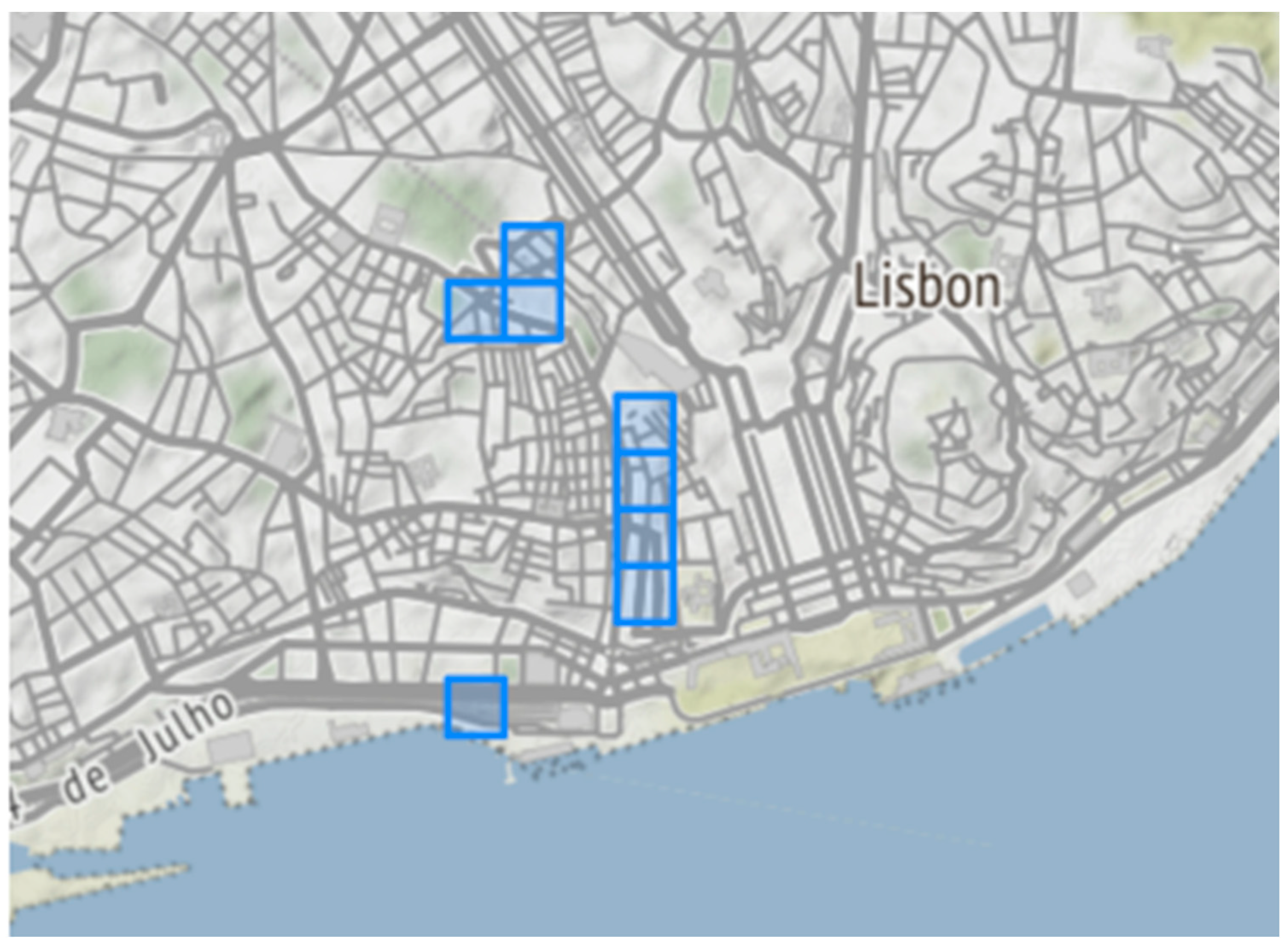
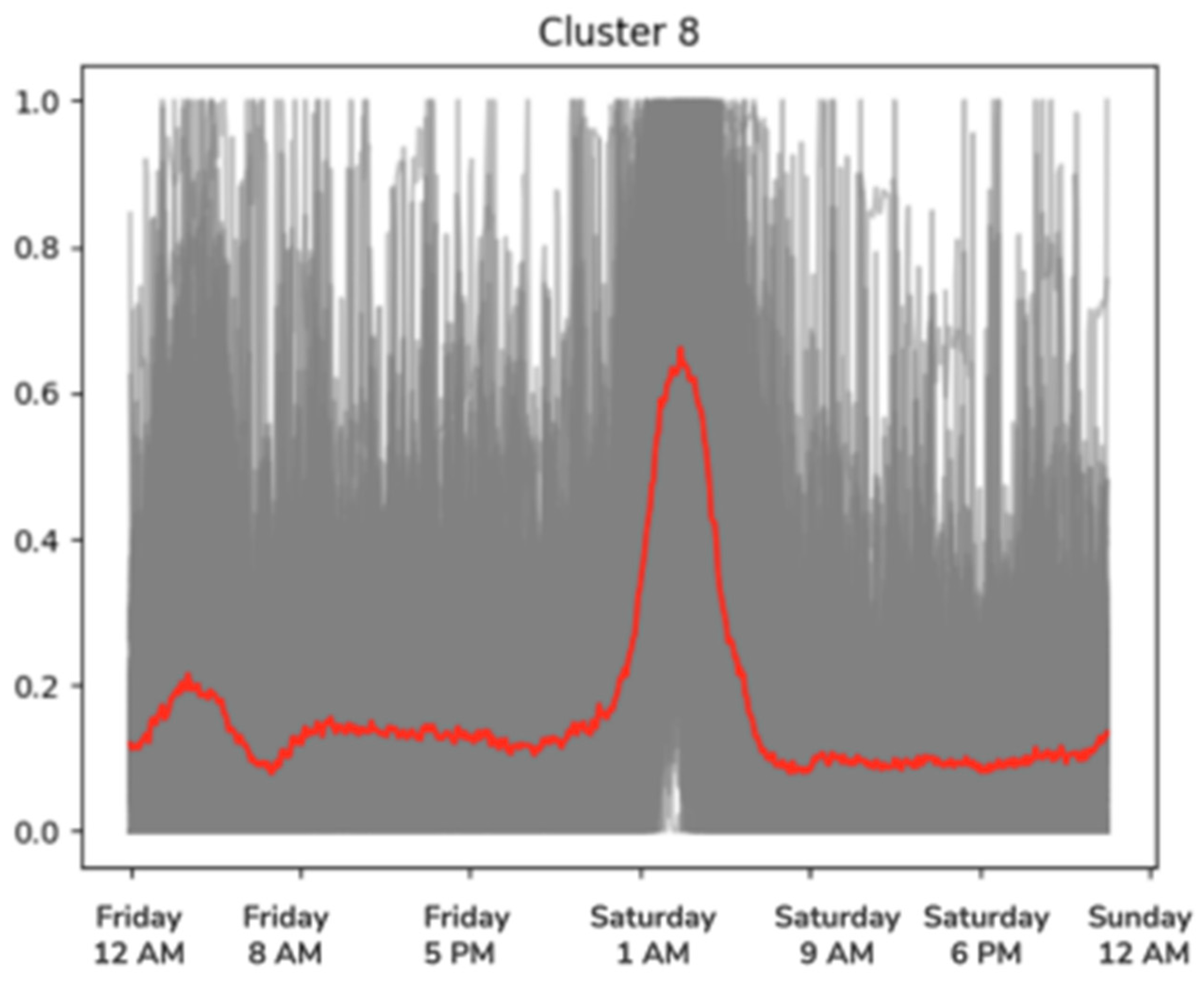
To give further perspective on how nightlife areas may vary, let us consider another cluster found by the algorithm, Cluster 8 (Figure 5). This cluster mainly encompasses the Santos dock area, where several nightclubs are located. This area consists mostly of night spots, a fact reflected by the map in Figure 5.
As is easily observed in Figure 6, there is one big spike in mobile phone entries after 1 a.m. Having insight into how the Lisbon nightlife behaves, this peak presumably correlates with a decrease in entries happening around the same time in the previously analyzed area, Bairro Alto, as people leave the smaller bars to spend the rest of the night in the more popular nightclubs. In comparison with Bairro Alto, the Santos dock area has very little touristic value, thus having a much smaller concentration of people during every other period outside of the peak.
In order to understand how tourists behave in the nightlife areas, a subsequent clustering was made, where the target variable was C2 (the number of distinct mobile phones in roaming in the grid), and only the time series corresponding to nightlife areas were included in the model. Once again, the SOM algorithm was used.
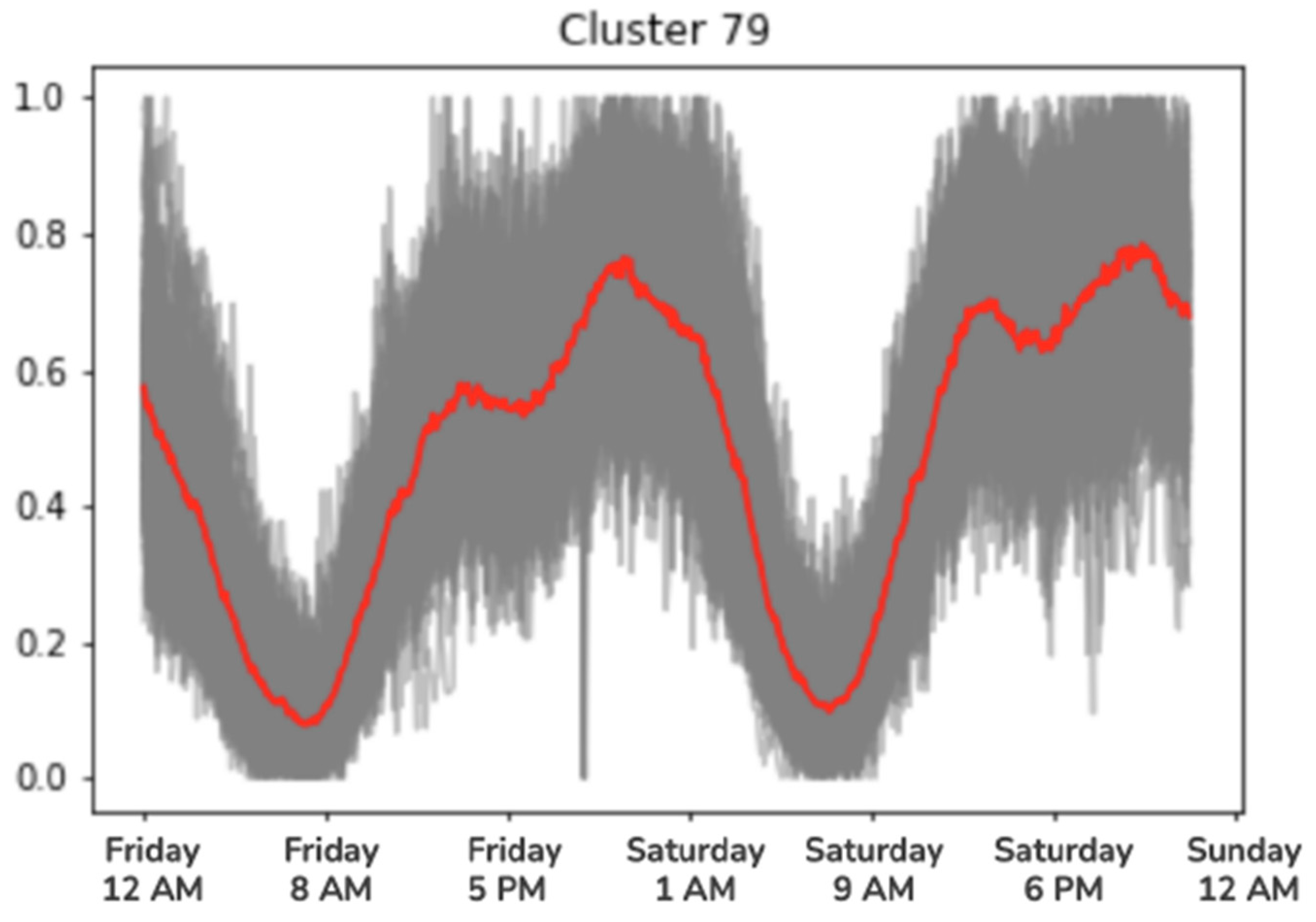
Figure 7 shows one of the clusters obtained from the C2 variable, Cluster 79. This cluster includes four grids referring to the Cais do Sodre and Rua do Alecrim area. Like Bairro Alto, this is an area with popular nightlife activity, depicted by the red line in Figure 8, where the C2 variable values are plotted between Friday 12 a.m. and Saturday 11:59 p.m. It can be observed that from Friday 8 a.m., there is an increase in mobile phones by grid, an ascending trend that continues until the maximum, which occurs around Saturday 1 a.m. This is quite reasonable, given that this is an area that has both tourist attractions and nightlife establishments. After 1 a.m. on Saturday, the values start to decrease, since, similarly to Bairro Alto, this is the time when people try to prolong the night in nightclubs or simply leave the area to go home. From 9 a.m. on Saturday, the Cais do Sodre area follows the trend of the previous day, once again showing demand from people of foreign nationality.
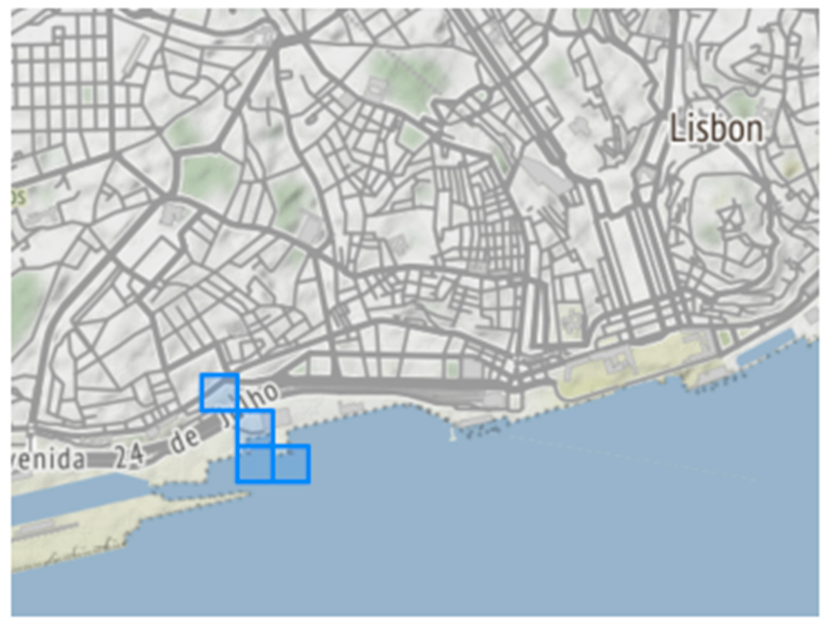
Another cluster that is worth analyzing is Cluster 70 (Figure 9), which refers to the Santos area (Cluster 70), more specifically, Cais da Viscondessa, where the K Urban Beach nightclub is located. Based on the trend of the red line in Figure 10, it can be assumed that this cluster corresponds to a grid containing nightclub-type establishments, as evidenced by the peak that can be observed in the early hours of Saturday. It is notable that from 1 a.m. on Saturday the trend is toward an increase of mobile phones in Cais da Viscondessa, prolonging until around Saturday at 3 a.m. From then, the tendency is to decrease until 9 a.m. on Saturday, during the period that tourists are leaving.
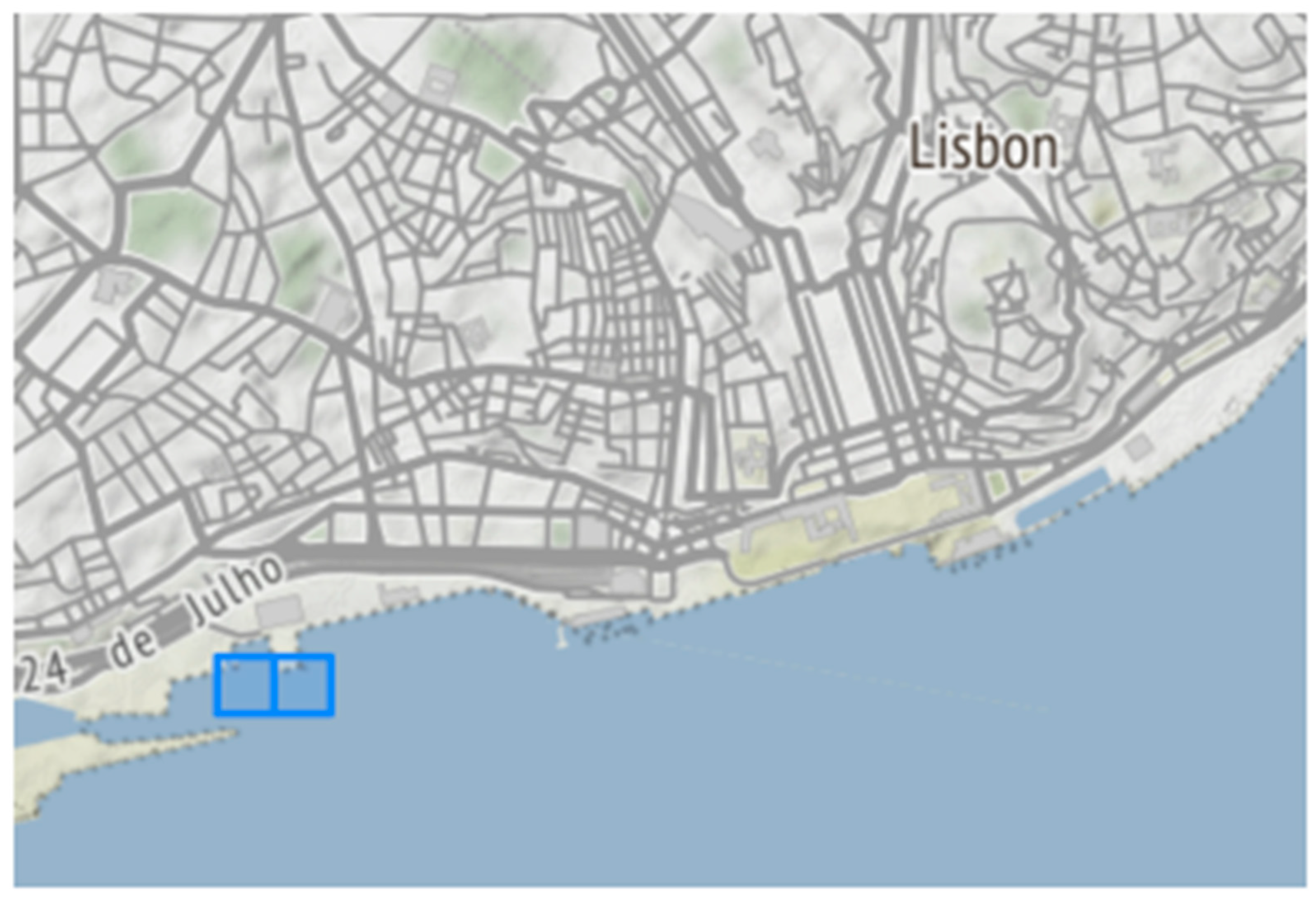
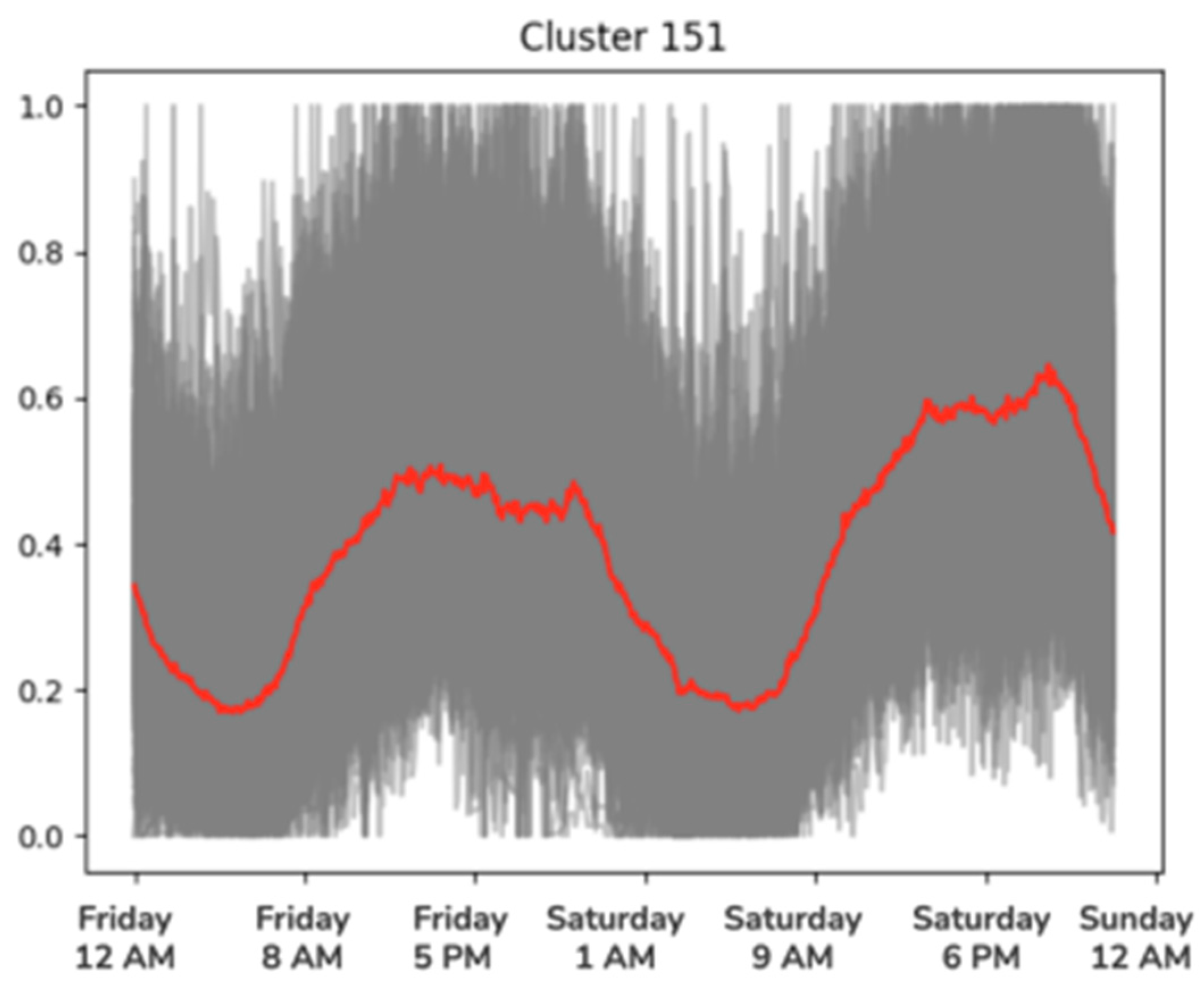
It is worth mentioning that the grids identified as nightlife areas have some flaws. One clear example of an area incorrectly recognized as a nightlife area is the Alfama area, with its corresponding grids in Figure 11.
As can be seen by the red trend line in Figure 12, there is a notable decrease in mobile phones around dinner time, which lasts the whole night and returns around Saturday at 9 a.m. This shows that this area does not offer much nightlife activity, despite containing many of the establishments present in the list provided by the City Council, which means that some of the entries in the list prevent the results from being even better. These may be restaurants that are open until late (thus being identified as nightlife establishments), as Alfama is a very touristic area. It is impossible to determine which establishments from the list limit the process, as each entry is composed solely by its latitude and longitude. A viable solution to this problem would be for the Lisbon City Council to provide a dataset with more information on each establishment.
4.2. Incorporating the Noise Data
In an attempt to further increase the accuracy of the obtained LSTM networks, we decided to try and include the noise data in the models.
The noise dataset was collected from the Lisbon City Council’s API3, where the noise level variable is identified as RULAEQ. There are a total of 80 sensors that measure this variable, and the data collected correspond to the hourly average of the noise level (in dB). These sensors were mostly placed on lampposts, and their locations were chosen with the purpose of collecting a diversified range of data [8].
Because of the large break in the mobile phone dataset, the noise data were collected for two separate periods: from September 2021 to January 2022, and from April to December 2022.
4.2.1. Data Pre-Processing
Unlike the mobile phone dataset, the noise data contained missing values: there were in 14,532 observations with the value −99. It was necessary to impute these values.
Within this analysis, the focus was on the noise sensors placed in nightlife areas. These correspond to RULAEQ0003, RULAEQ0005, RULAEQ0012, RULAEQ0014, RULAEQ0017, RULAEQ0076, RULAEQ0077, which can be found in Figure 13.
Having discarded all other sensors from the dataset, it was then discovered that many periods were also missing entirely, instead of being identified with an NaN value. It was therefore necessary to identify every missing period and add it to the dataset to prevent breaks in the time series (similar to the process for the mobile phone dataset).
Lastly, it was necessary to prepare the noise data for them to be comparable with the number of mobile phones in a given grid (C1 variable). The noise data in our study were averaged hourly, while mobile phone counts were recorded every 5 min. This difference in time intervals created a mismatch between the datasets. To address this, we inserted timestamps for each 5-min interval between two consecutive hourly noise measurements. Subsequently, we imputed the missing noise values for these newly added timestamps. This step ensured that both datasets were aligned in terms of timing, facilitating a more coherent analysis.
4.2.2. Relationship between Noise Levels and the Number of People
The methodology to identify the relationship between the noise levels and number of people on a nightlife grid proceeded as follows:
- Divide the noise dataset into periods of 48 h, and save those that start on a Friday and end on a Saturday (similar to with the process for the primary dataset in Section 4);
- Plot every saved time series, and add the corresponding time series of the C1 variable (after both have been normalized);
- Analyze the Pearson’s correlation coefficient between the two curves.
The Pearson’s correlation coefficient measures the direction and the strength of the linear relationship between two given variables, in this case, the number of mobile phones, and the noise levels. Its values can range from −1 to 1, where positive values indicate that the increase in one variable is followed by an increase in the other, and negative values indicate that the increase is followed by a decrease. Zero means that the relationship between the two variables is non-existent, and the closer the coefficient is to 1 (or −1), the greater the impact a variable has on the other.
The expectation is for the coefficient values to be high and positive, meaning that great noise levels are associated with large concentrations of people. Table 3 shows the descriptive statistics of the coefficients obtained for every sensor in each Friday–Saturday period.
On average, the only sensors whose noise levels are moderately correlated with the number of mobile phones are RULAEQ0014 and RULAEQ0077, with some values showing strong correlations (greater than 0.7), and the standard deviation being relatively low. RULAEQ0076 shows an average weak correlation, and the remaining sensors show negligible means (the fact that there are high max and minimum values shows that there is no consistency in the direction of the relationship; thus, the average coefficient is close to zero).
The reason for these values has mostly to do with the location of the sensors. In general, those with high correlations are placed in areas with a lot of pedestrians, and those with low correlations are located in areas with a lot of car traffic. This reflects Lisbon City Council’s strategy of collecting a wide variety of data.
Figure 14 shows an example of a strong correlation, whereas Figure 15 shows one that is weak. In the plot of RULAEQ0077, it is evident that the increase in noise is closely related to the increase in the number of people. On the other hand, the plot of RULAEQ0076 shows that an increase in the noise levels may not necessarily lead to an increase in the number of people.
The low average coefficients do not necessarily indicate that the noise levels will not improve the accuracy of the LSTM models. Given the max and minimum values in Table 3, one can see that there were often moderate (or even high) correlation coefficients, but the correlations are not consistent, with this inconsistency caused by some factors that the LSTM model may identify and use to improve its forecasts. This potential for the noise levels is evident in Figure 15. The increase in the noise levels in the first half is not matched with an increase in the number of people, but the sudden decrease is strongly correlated with the decrease in the number of people.
4.3. Noise Levels in the Forecasting
Having concluded that there are some strong correlations between the noise levels and the number of mobile phones in a nightlife area, the possibility arose that the noise levels in the LSTM models could increase the accuracy of their forecasts. Therefore, the areas of the city with noise sensors were identified, and their neural networks were fitted again. The results based on the test set can be seen in Table 4, where they are compared with the results obtained without the inclusion of the noise levels.
The only sensor that significantly increased the accuracy of the model was RULAEQ0005, with the RMSE (root mean square error) on the test set decreasing by five units in that area (there was also a decrease in the RMSE on the train and validation set). It can also be noted that the MAPE increased by 0.033 percentage points, from 11.395 to 11.428. As these two errors contradict each other, the choice was made to rely on the findings of the RMSE, as that is the error the model was trained on, and the dataset is the same for both models. The choice to rely on the RMSE is the reason that we concluded that sensor RULAEQ0076 did not improve the accuracy of the model, despite the fact that the MAPE decreased by 0.120 percentage points. Comparing these results with the Pearson’s correlation coefficients in Table 3, it can be observed that high correlations to noise levels do not necessarily increase the accuracy of the forecasts (in the context of these LSTM networks). In fact, the only model that had an increase in its accuracy corresponds to a noise level sensor with one of the lowest means in correlation degree. The fact that there was an increase in the accuracy of one LSTM network shows that relocating the noise sensors to more appropriate locations should lead to big increases in the accuracy of the neural networks in general.
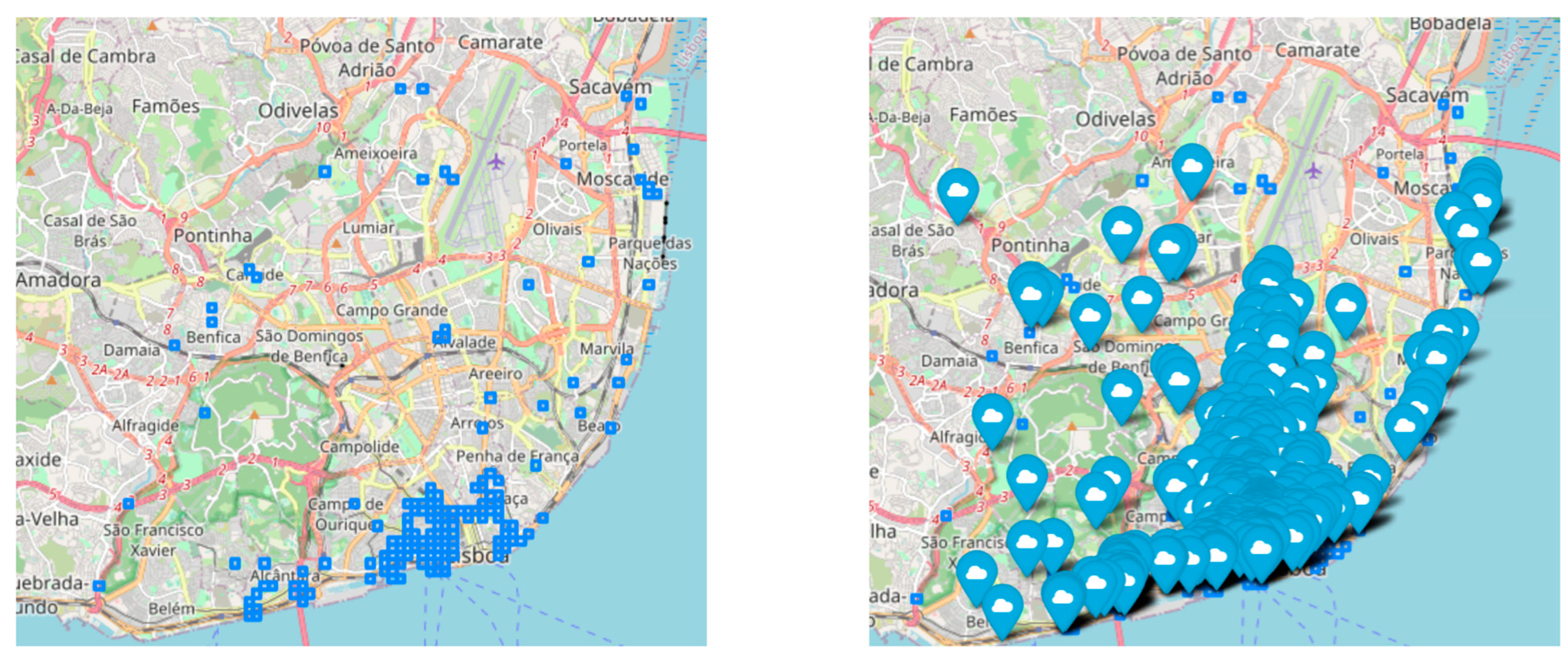
When comparing the night establishments identified by Lisbon municipality with the clusters identified by the algorithm, it is noticeable that there is an overlap between the location of such establishments and the clusters, as depicted in Figure 16.
5. Conclusions
This study has demonstrated the feasibility and significance of using mobile phone data for the analysis of nocturnal urban noise patterns and the identification of distinct noise zones within a city. The integration of mobile phone technology, machine learning, and soundscape analysis has opened up new avenues for comprehensively understanding and managing urban noise pollution.
Through the analysis of audio recordings collected from mobile phones placed across various urban areas during nighttime hours, it has been possible to capture the dynamic nature of urban soundscapes. The extracted noise features, combined with geographic location data, have facilitated the creation of detailed noise maps that reflect the varying intensities and sources of noise pollution. These noise maps provide a richer representation of the urban environment, enabling more informed decision making for urban planning and noise mitigation strategies.
The application of clustering algorithms to the combined audio and location data allows us to delineate distinct noise zones within the city. These noise zones capture the heterogeneity of noise sources and their distribution, shedding light on areas with varying levels of noise pollution. This information is invaluable for urban planners, policy makers, and public health officials seeking to design targeted interventions that enhance quality of life for city residents.
However, it is essential to acknowledge the challenges inherent in this approach. Ensuring the quality and accuracy of mobile phone-generated noise data remains a critical consideration. Privacy concerns and representativeness of the data are areas that require careful attention to ensure the credibility and validity of the findings.
In essence, this research showcases the transformative potential of mobile phone data in the field of noise analysis and urban planning. By integrating this innovative approach into existing noise management strategies, cities can move towards more adaptive and data-driven policies, resulting in healthier and more livable urban environments. As cities continue to grow and evolve, the ability to harness technology to gain a deeper understanding of their sonic landscapes will play a pivotal role in shaping the future of urban living. This study provides a stepping stone towards that future, contributing to the body of knowledge that underpins sustainable and harmonious urban development.
Author Contributions
Conceptualization, B.F. and L.B.E.; methodology, L.B.E.; software, M.N.; validation, J.A.A.; data curation, L.B.E. and M.N.; writing—original draft preparation, B.F. and J.C.F.; writing—review and editing, J.A.A. and J.C.F.; supervision, J.C.F. and B.F. All authors have read and agreed to the published version of the manuscript.
Funding
This work was supported by the Fundação para a Ciência e Tecnologia under Grant [UIDB/00315/2020]; and by the project “BLOCKCHAIN.PT (RE-C05-i01.01—Agendas/Alianças Mobilizadoras para a Reindustrialização, Plano de Recuperação e Resiliência de Portugal” in its component 5—Capitalization and Business Innovation and with the Regulation of the Incentive System “Agendas for Business Innovation”, approved by Ordinance No. 43-A/2022 of 19 January 2022).
Institutional Review Board Statement
Not applicable.
Data Availability Statement
Restrictions apply to the availability of these data. Data was obtained from [third party] and are available [Lisbon Municipality/at https://lisboaaberta.cm-lisboa.pt/index.php/pt/lx-data-lab/desafios] with the permission of Lisbon Municipality.
Acknowledgments
EEA Grants Blue Growth Programme (Call #5), Project PT-INNOVATION-0069-Fish2Fork.
Conflicts of Interest
The authors declare no conflicts of interest.
References
- Wu, K.; Wang, R.; Zhang, Y.; Wu, R.; He, Y.; Li, B.; Zhang, Y. The Influence of New-Type Urbanization and Environmental Pollution on Public Health: A Spatial Durbin Model Study. Sustainability 2023, 15, 16144. [Google Scholar] [CrossRef]
- Jariwala, H.; Syed, H.; Pandya, M.; Gajera, Y. Conference: Noise and Air Pollution: Challenges and Opportunities, Noise Pollution & Human Health: A Review. 2017. Available online: https://www.researchgate.net/profile/Hiral-Jariwala/publication/319329633_Noise_Pollution_Human_Health_A_Review/links/59a54434a6fdcc773a3b1c49/Noise-Pollution-Human-Health-A-Review.pdf (accessed on 24 October 2023).
- Sun, C.; Wang, Y.; Zhu, Z. Urbanization and residents’ health: From the perspective of environmental pollution. Environ. Sci. Pollut. Res. Int. 2023, 30, 67820–67838. [Google Scholar] [CrossRef] [PubMed]
- Asdrubali, F.; D’alessandro, F. Innovative Approaches for Noise Management in Smart Cities: A Review. Curr. Pollut. Rep. 2018, 4, 143–153. [Google Scholar] [CrossRef]
- Pita, A.; Rodriguez, F.J.; Navarro, J.M. Cluster Analysis of Urban Acoustic Environments on Barcelona Sensor Network Data. Int. J. Environ. Res. Public. Health 2021, 18, 8271. [Google Scholar] [CrossRef] [PubMed]
- Fredianelli, L.; Carpita, S.; Bernardini, M.; Del Pizzo, L.G.; Brocchi, F.; Bianco, F.; Licitra, G. Traffic Flow Detection Using Camera Images and Machine Learning Methods in ITS for Noise Map and Action Plan Optimization. Sensors 2022, 22, 1929. [Google Scholar] [CrossRef]
- Alías, F.; Alsina-Pagès, R.M. Review of Wireless Acoustic Sensor Networks for Environmental Noise Monitoring in Smart Cities. J. Sens. 2019, 2019, e7634860. [Google Scholar] [CrossRef]
- Liu, Y.; Ma, X.; Shu, L.; Yang, Q.; Zhang, Y.; Huo, Z.; Zhou, Z. Internet of Things for Noise Mapping in Smart Cities: State of the Art and Future Directions. IEEE Netw. 2020, 34, 112–118. [Google Scholar] [CrossRef]
- López, J.M.; Alonso, J.; Asensio, C.; Pavón, I.; Gascó, L.; de Arcas, G. A Digital Signal Processor Based Acoustic Sensor for Outdoor Noise Monitoring in Smart Cities. Sensors 2020, 20, 605. [Google Scholar] [CrossRef]
- Licitra, G.; Artuso, F.; Bernardini, M.; Moro, A.; Fidecaro, F.; Fredianelli, L. Acoustic Beamforming Algorithms and Their Applications in Environmental Noise. Curr. Pollut. Rep. 2023, 9, 486–509. [Google Scholar] [CrossRef]
- Ballesteros, J.A.; Sarradj, E.; Fernández, M.D.; Geyer, T.; Ballesteros, M.J. Noise source identification with Beamforming in the pass-by of a car. Appl. Acoust. 2015, 93, 106–119. [Google Scholar] [CrossRef]
- Bolognese, M.; Carpita, S.; Fredianelli, L.; Licitra, G. Definition of Key Performance Indicators for Noise Monitoring Networks. Environments 2023, 10, 61. [Google Scholar] [CrossRef]
- Ascari, E.; Cerchiai, M.; Fredianelli, L.; Licitra, G. Statistical Pass-By for Unattended Road Traffic Noise Measurement in an Urban Environment. Sensors 2022, 22, 8767. [Google Scholar] [CrossRef] [PubMed]
- Pallas, M.-A.; Bérengier, M.; Chatagnon, R.; Czuka, M.; Conter, M.; Muirhead, M. Towards a model for electric vehicle noise emission in the European prediction method CNOSSOS-EU. Appl. Acoust. 2016, 113, 89–101. [Google Scholar] [CrossRef]
- Licitra, G.; Bernardini, M.; Moreno, R.; Bianco, F.; Fredianelli, L. CNOSSOS-EU coefficients for electric vehicle noise emission. Appl. Acoust. 2023, 211, 109511. [Google Scholar] [CrossRef]
- Steinbach, L.; Altinsoy, M.E. Prediction of annoyance evaluations of electric vehicle noise by using artificial neural networks. Appl. Acoust. 2019, 145, 149–158. [Google Scholar] [CrossRef]
- Shah, S.K.; Tariq, Z.; Lee, J.; Lee, Y. Real-Time Machine Learning for Air Quality and Environmental Noise Detection. In Proceedings of the IEEE International Conference on Big Data (Big Data), Atlanta, GA, USA, 10–13 December 2020; pp. 3506–3515. [Google Scholar] [CrossRef]
- Nourani, V.; Gökçekuş, H.; Umar, I.K. Artificial intelligence based ensemble model for prediction of vehicular traffic noise. Environ. Res. 2020, 180, 108852. [Google Scholar] [CrossRef]
- Renaud, J.; Karam, R.; Salomon, M.; Couturier, R. Deep learning and gradient boosting for urban environmental noise monitoring in smart cities. Expert Syst. Appl. 2023, 218, 119568. [Google Scholar] [CrossRef]
- Goggin, G.; Clark, J. Mobile phones and community development: A contact zone between media and citizenship. Dev. Pract. 2009, 19, 585–597. [Google Scholar] [CrossRef]
- Zuo, J.; Xia, H.; Liu, S.; Qiao, Y. Mapping Urban Environmental Noise Using Smartphones. Sensors 2016, 16, 1692. [Google Scholar] [CrossRef] [PubMed]
- Longo, A.; Zappatore, M.; Bochicchio, M.; Navathe, S.B. Crowd-Sourced Data Collection for Urban Monitoring via Mobile Sensors. ACM Trans. Internet Technol. 2017, 18, 5:1–5:21. [Google Scholar] [CrossRef]
- Arshi, O.; Mondal, S. Advancements in sensors and actuators technologies for smart cities: A comprehensive review. Smart Constr. Sustain. Cities 2023, 1, 18. [Google Scholar] [CrossRef]
- Page, M.J.; McKenzie, J.E.; Bossuyt, P.M.; Boutron, I.; Hoffmann, T.C.; Mulrow, C.D.; Shamseer, L.; Tetzlaff, J.M.; Akl, E.A.; Brennan, S.E.; et al. The PRISMA 2020 statement: An updated guideline for reporting systematic reviews. BMJ 2021, 372, n71. [Google Scholar] [CrossRef] [PubMed]
- Albaji, A.O.; Rashid, R.B.A.; Hamid, S.Z.A. Investigation on Machine Learning Approaches for Environmental Noise Classifications. J. Electr. Comput. Eng. 2023, 2023, 3615137. [Google Scholar] [CrossRef]
- Toutouh, J.; Alba, E. A Low Cost IoT Cyber-Physical System for Vehicle and Pedestrian Tracking in a Smart Campus. Sensors 2022, 22, 6585. [Google Scholar] [CrossRef] [PubMed]
- Bhoi, S.K.; Mallick, C.; Mohanty, C.R.; Nayak, R.S. Analysis of Noise Pollution during Dussehra Festival in Bhubaneswar Smart City in India: A Study Using Machine Intelligence Models. Appl. Comput. Intell. Soft Comput. 2022, 2022, 6095265. [Google Scholar] [CrossRef]
- Middya, A.; Roy, S.; Dutta, J.; Das, R. JUSense: A Unified Framework for Participatory-based Urban Sensing System. Mob. Netw. Appl. 2020, 25, 1249–1274. [Google Scholar] [CrossRef]
- Chaware, S.; Chaware, T. Proposed algorithm for smart traffic control using ultrasonic sensors. Int. J. Eng. Adv. Technol. 2019, 8, 3912–3915. [Google Scholar] [CrossRef]
- Hernandez-Jayo, U.; Goñi, A. Zaratamap: Noise characterization in the scope of a smart city through a low cost and mobile electronic embedded system. Sensors 2021, 21, 1707. [Google Scholar] [CrossRef]
- Kaarivuo, A.; Salo, K.; Mikkonen, T. From sonic experiences to urban planning innovations. Eur. Plan. Stud. 2021, 34, 4. [Google Scholar] [CrossRef]
- Zamora, W.; Vera, E.; Calafate, C.T.; Cano, J.-C.; Manzoni, P. GRC-sensing: An architecture to measure acoustic pollution based on crowdsensing. Sens. Switz. 2018, 18, 2596. [Google Scholar] [CrossRef]
- Monti, L.; Vincenzi, M.; Mirri, S.; Pau, G.; Salomoni, P. Raveguard: A noise monitoring platform using low-end microphones and machine learning. Sensors 2020, 20, 5583. [Google Scholar] [CrossRef] [PubMed]
- Middya, A.; Roy, S. Spatial Interpolation Techniques on Participatory Sensing Data. ACM Trans. Spat. Algorithms Syst. 2021, 7, 1–32. [Google Scholar] [CrossRef]
- Shen, Y.; Cao, J.; Wang, J.; Yang, Z. Urban acoustic classification based on deep feature transfer learning. J. Frankl. Inst.-Eng. Appl. Math. 2020, 357, 667–686. [Google Scholar] [CrossRef]
- Lebrusan, I.; Toutouh, J. Using Smart City Tools to Evaluate the Effectiveness of a Low Emissions Zone in Spain: Madrid Central. Smart Cities 2020, 3, 456–478. [Google Scholar] [CrossRef]
- Navarro, J.M.; Martínez-España, R.; Bueno-Crespo, A.; Martínez, R.; Cecilia, J.M. Sound levels forecasting in an acoustic sensor network using a deep neural network. Sens. Switz. 2020, 20, 903. [Google Scholar] [CrossRef]
- Zhang, X.; Kuehnelt, H.; De Roeck, W. Traffic noise prediction applying multivariate bi-directional recurrent neural network. Appl. Sci. Switz. 2021, 11, 2714. [Google Scholar] [CrossRef]
- Awan, F.M.; Minerva, R.; Crespi, N. Using Noise Pollution Data for Traffic Prediction in Smart Cities: Experiments Based on LSTM Recurrent Neural Networks. IEEE Sens. J. 2021, 21, 20722–20729. [Google Scholar] [CrossRef]
Figure 1.
PRISMA workflow diagram.

Figure 2.
Nightlife areas identified in the city of Lisbon (represented by the blue squares).

Figure 3.
Grids corresponding to Cluster 165, the Bairro Alto area.

Figure 4.
Time series for Cluster 165.

Figure 5.
Grids corresponding to Cluster 8, the Santos dock area.

Figure 6.
Time series for Cluster 8.

Figure 7.
Grids corresponding to Cluster 79, the Cais do Sodre area.

Figure 8.
Time series for Cluster 79.

Figure 9.
Grids corresponding to Cluster 70, the Cais da Viscondessa area.

Figure 10.
Time series for Cluster 70.

Figure 11.
Grids corresponding to Cluster 151, the Alfama area.

Figure 12.
Cluster 151, the Alfama area.

Figure 13.
Noise sensors and their respective locations, where the clouds represent the sensors and the squares represent the clusters identified by the algorithm with more people.
Figure 13.
Noise sensors and their respective locations, where the clouds represent the sensors and the squares represent the clusters identified by the algorithm with more people.

Figure 14.
Strong correlation between the noise sensor and the number of mobile phones.

Figure 15.
Weak correlation between the noise sensor and the number of mobile phones.

Figure 16.
The map on the left shows the clusters identified by the algorithm as “nightlife”, and the map on the right shows the overlap between the clusters and nightlife establishments (represented by the pins).
Figure 16.
The map on the left shows the clusters identified by the algorithm as “nightlife”, and the map on the right shows the overlap between the clusters and nightlife establishments (represented by the pins).


Table 1.
Topics found in the literature review.
| Topic | References | Number of Documents |
|---|---|---|
| Machine Learning | [25,26,27,28,29,30,31,32,33] | 9 |
| Noise Pollution | [25,26,27,28,29,33,34,35,36] | 9 |
| Noise Monitoring | [8,19,30,31,32,33,34] | 7 |
| Internet of Things | [8,26,28,33,34,37] | 6 |
| Deep Learning | [19,35,37,38,39] | 5 |
| Smart Traffic | [29,36,39] | 3 |
| Noise Prediction | [27,37,38] | 2 |
Table 2.
Description of each variable present in the main dataset files.
| Variable | Description |
|---|---|
| Grid_ID | Identification of the grid cell number |
| Datetime | Date and time |
| extract_year_2 | Year |
| extract_month_3 | Month |
| extract_day_4 | Day |
| C1 | Number of distinct terminals in the grid, during the 5 min |
| C2 | Number of distinct terminals, roaming, in the grid, during the 5 min |
| C3 | Number of distinct terminals remaining in the grid at the end of each 5 min |
| C4 | Number of distinct terminals remaining in the grid, roaming, at the end of each 5 min |
| C5 | Number of distinct terminal entries in the grid |
| C6 | The number of distinct terminals exits in the grid |
| C7 | Number of distinct terminal entries in the grid, roaming |
| C8 | Number of distinct terminals exits in the grid, roaming |
| C9 | Number of distinct terminals with an active data connection, in the grid cell, during the 5 min |
| C10 | Number of distinct terminals with an active data connection, roaming, in the grid cell, during the 5 min |
| C11 | Number of voice calls originating from the grid |
| C12 | Number of entries into Lisbon along the 11 main roads |
| C13 | Number of exits into Lisbon along the 11 main roads |
| D1 | Top 10 home countries of terminal equipment roaming |
| E1 | Number of voice calls terminated in the grid |
| E2 | The average downstream rhythm of the grid |
| E3 | The average upstream rhythm of the grid |
| E4 | Peak downstream rhythm of the grid |
| E5 | Peak upstream rhythm of the grid |
| E6 | Top 10 apps (semicolon separated) |
| E7 | Duration of the minimum stay within the grid |
| E8 | Duration of the average stay within the grid |
| E9 | Duration of the maximum stay within the grid |
| E10 | Number of devices performing grid connection sharing during the 5 min |
Table 3.
Descriptive statistics of the Pearson’s correlation coefficients.
| Sensor | Max | Min | Mean | Standard Deviation |
|---|---|---|---|---|
| RULAEQ0003 | 0.498 | 0.222 | 0.167 | 0.195 |
| RULAEQ0005 | 0.145 | 0.316 | 0.136 | 0.134 |
| RULAEQ0012 | 0.462 | 0.548 | 0.072 | 0.256 |
| RULAEQ0014 | 0.796 | 0.210 | 0.561 | 0.128 |
| RULAEQ0017 | 0.589 | 0.186 | 0.176 | 0.184 |
| RULAEQ0076 | 0.697 | 0.111 | 0.354 | 0.159 |
| RULAEQ0077 | 0.803 | 0.289 | 0.636 | 0.130 |
Table 4.
Results of the original models compared with those obtained with noise levels.
| Sensor | Grid | RMSE (Noise) | RMSE (Before) | MAPE (Noise) | MAPE (Before) |
|---|---|---|---|---|---|
| 3 | 304 | 37.709 | 35.982 | 34.297 | 33.425 |
| 5 | 344 | 110.499 | 115.830 | 11.428 | 11.395 |
| 12 | 678 | 87.696 | 86.607 | 11.185 | 11.022 |
| 14 | 746 | 92.086 | 90.762 | 7.776 | 7.536 |
| 17 | 796 | 60.614 | 58.445 | 10.283 | 9.989 |
| 76 | 742 | 80.196 | 78.757 | 10.713 | 10.833 |
| 77 | 624 | 41.835 | 41.853 | 17.254 | 17.359 |
Disclaimer/Publisher’s Note: The statements, opinions and data contained in all publications are solely those of the individual author(s) and contributor(s) and not of MDPI and/or the editor(s). MDPI and/or the editor(s) disclaim responsibility for any injury to people or property resulting from any ideas, methods, instructions or products referred to in the content. |
© 2023 by the authors. Licensee MDPI, Basel, Switzerland. This article is an open access article distributed under the terms and conditions of the Creative Commons Attribution (CC BY) license (https://creativecommons.org/licenses/by/4.0/).
Share and Cite
MDPI and ACS Style
Elvas, L.B.; Nunes, M.; Ferreira, J.C.; Francisco, B.; Afonso, J.A. Georeferenced Analysis of Urban Nightlife and Noise Based on Mobile Phone Data. Appl. Sci. 2024, 14, 362. https://0-doi-org.brum.beds.ac.uk/10.3390/app14010362
AMA Style
Elvas LB, Nunes M, Ferreira JC, Francisco B, Afonso JA. Georeferenced Analysis of Urban Nightlife and Noise Based on Mobile Phone Data. Applied Sciences. 2024; 14(1):362. https://0-doi-org.brum.beds.ac.uk/10.3390/app14010362
Chicago/Turabian StyleElvas, Luís B., Miguel Nunes, Joao C. Ferreira, Bruno Francisco, and Jose A. Afonso. 2024. "Georeferenced Analysis of Urban Nightlife and Noise Based on Mobile Phone Data" Applied Sciences 14, no. 1: 362. https://0-doi-org.brum.beds.ac.uk/10.3390/app14010362
Note that from the first issue of 2016, this journal uses article numbers instead of page numbers. See further details here.