
Bearing Fault Diagnosis Based on Image Information Fusion and Vision Transformer Transfer Learning Model


1
School of Mechanical and Equipment Engineering, Hebei University of Engineering, Handan 056038, China
2
School of Mining and Geomatics Engineering, Hebei University of Engineering, Handan 056038, China
*
Author to whom correspondence should be addressed.
Appl. Sci. 2024, 14(7), 2706; https://0-doi-org.brum.beds.ac.uk/10.3390/app14072706
Submission received: 7 March 2024
/
Revised: 21 March 2024
/
Accepted: 22 March 2024
/
Published: 23 March 2024
(This article belongs to the Collection Bearing Fault Detection and Diagnosis)
Abstract
:In order to improve the accuracy of bearing fault diagnosis under a small sample, variable load, and noise conditions, a new fault diagnosis method based on an image information fusion and Vision Transformer (ViT) transfer learning model is proposed in this paper. Firstly, the method applies continuous wavelet transform (CWT), Gramian angular summation field (GASF), and Gramian angular difference field (GADF) to the time series data, and generates three grayscale images. Then, the generated three grayscale images are merged into an information fusion image (IFI) using image processing techniques. Finally, the obtained IFIs are fed into the advanced ViT model and trained based on transfer learning. In order to verify the effectiveness and superiority of the proposed method, the rolling bearing dataset from Case Western Reserve University (CWRU) is used to carry out experimental studies under different working conditions. Experimental results show that the method proposed in this paper is superior to other traditional methods in terms of accuracy, and the effect of ViT model based on transfer learning (TLViT) training is better than that of the Resnet50 model based on transfer learning training (TLResnet50) under variable loads and small sample conditions. In addition, the experimental results also prove that the IFI with multiple image information has better anti-noise ability than the single information image. Therefore, the method proposed in this paper can improve the accuracy of bearing fault diagnosis under small sample, variable load and noise conditions, and provide a new method for bearing fault diagnosis.
1. Introduction
In the process of industrial production, bearing failure is one of the common causes of mechanical equipment failure. Bearing status directly affects the operation of the whole rotating machinery; the existence of bearing failure will reduce the reliability and availability of equipment. Therefore, the timely diagnosis of bearing is of great significance in the current mechanical equipment maintenance and health management [1]. The traditional bearing fault diagnosis method mainly relies on manual experience and professional knowledge, but this method has some problems, such as time consumption, power consumption, and being easy to be affected by subjective factors. With the continuous progress of science and technology, the application of machine learning and artificial intelligence in various fields is more and more extensive, and has attracted wide attention. In recent years, with the continuous development of computer computing power, deep learning models with strong data-mining ability have been widely used in the field of fault diagnosis [2]. In the research of bearing fault diagnosis based on a machine learning model, Song et al. [3] used Wavelet Packet Transform (WPT) to decompose bearing vibration signals, and then used a Support vector machine (SVM) to carry out fault diagnosis. Zhu et al. [4] presents a fault diagnosis method based on wavelet threshold (WT), variational mode decomposition (VMD), and random forest. Amarnath et al. [5] extracted features from sound signals, reduced the dimensionality of features through Decision Trees to select important features, and then used a C4.5 Decision Tree algorithm to classify the selected features and complete fault diagnosis. In order to build models and process features, these machine learning methods all require certain prior knowledge and assumptions, and this method of manually extracting features has great limitations.
Deep learning has strong feature-learning ability and does not need to rely on manual feature extraction, so it has received great attention and has been widely used in the field of fault diagnosis. Fuan et al. [6] applied Convolutional Neural Network (CNN) to the fault diagnosis of rolling bearing. Eren et al. [7] proposed an adaptive one-dimensional CNN classification method which combined the feature extraction and classification blocks of the traditional mode into a special structure, learned the best features from the original vibration signals of bearing, and achieved a high degree of generalization. Song et al. [8] adopted the strategy of expanding a convolution kernel to obtain a larger receptive field, and the proposed model has good performance in terms of accuracy, noise resistance, and timeliness. For multi-channel data, Guo et al. [9] proposed a method for fault diagnosis using dimensionality reduction in multi-line subspace and then used CNN to extract fault features. Liu et al. [10] proposed a new bearing fault diagnosis algorithm based on the combination of Sparse Wavelet Decomposition and multi-scale one-dimensional CNN (1-DCNN), they used convolution kerns of different sizes to extract signal features from multiple scales. The original vibration signal of bearing is a kind of time sequence signal, and the CNN model cannot process the time information in the signal, so the recurrent neural network (RNN) sensitive to the time sequence characteristics has been widely used in the field of bearing fault diagnosis. Liu et al. [11] proposed a bearing fault diagnosis method based on RNN. A Long-Shot Term Memory (LSTM) network is a variant of an RNN that can solve the difficulty of RNN convergence and the disappearance of gradients. Zou et al. [12] combined signal processing technology with LSTM network to realize fault diagnosis in the case of small sample size. In order to combine the ability of CNN to extract spatial features and the sensitivity of LSTM to time series information, Pan et al. [13] used the series structure of 1D-CNN and LSTM to realize bearing fault diagnosis, and the diagnosis accuracy was higher than that of the single 1D-CNN model and LSTM model. However, for a too-long time series, LSTM is still prone to gradient disappearance and gradient explosion in the calculation process, and because of the cyclic structure of LSTM model, it is difficult to carry out effective parallel calculation.
The above methods are all proposed based on the original one-dimensional vibration signal data. At present, more and more scholars are beginning to convert one-dimensional data into two-dimensional images and make use of the advantages of deep learning models in the field of computer vision to achieve better diagnosis results. Hoang et al. [14] converted one-dimensional vibration signals into two-dimensional gray images and sent the images into CNN for bearing fault diagnosis, making full use of the advantages of CNN that are good at extracting image features and achieving better diagnosis results. Zhou et al. [15] directly took the bearing vibration waveform as the two-dimensional image input of the CNN model to obtain better real-time performance. Wen et al. [16] proposed a new method to transform one-dimensional data into a two-dimensional image without any predefined parameters, eliminating the influence of expert’s knowledge as much as possible. The image was trained in the LeNet-5 model based on CNN, and the proposed method which was tested on three famous datasets, including motor bearing dataset, self-priming centrifugal pump dataset, and axial piston hydraulic pump dataset, and had achieved a prediction accuracy of 99.79%, 99.481%, and 100%, respectively. Luo et al. [17] utilized the Adaptive Optimal-Kernel Time-Frequency Representation (AOK-TFR) algorithm to transform time series into time-frequency spectrogram representations, thereby simultaneously capturing signal characteristics from both time and frequency domains.
In recent years, researchers have introduced attention mechanisms into deep learning to address the drawbacks of traditional models, such as high complexity, large number of parameters, and high computational cost. The attention mechanism is derived from human visual attention and can automatically learn to focus on different parts of the input, thus enhancing the performance of the model. Through this approach, the model can better comprehend the intrinsic structure and semantic information of the input data. Introducing attention mechanism into deep learning models for fault diagnosis tasks has also become a research trend. Guo et al. [18] proposed an attention-based CNN-BiLSTM network, which achieved a diagnosis accuracy of 96.58% even under noisy conditions. Yang et al. [19] introduced a multi-scale feature fusion CNN with an attention mechanism for bearing fault diagnosis. Common methods used to convert one-dimensional vibration signals into two-dimensional images include continuous wavelet transform (CWT) [20], short-time Fourier transform (STFT) [21], and Gramian angular field (GAF) [22]. Among them, CWT and STFT are both time-frequency analysis methods, which transform signals from the time domain to the frequency domain for analysis. CWT enables multi-scale analysis of signals, thereby providing more detailed information in both time and frequency domains, making it suitable for analyzing non-stationary signals. Compared to STFT, CWT has better capability to capture the local time-frequency features of a signal, allowing for a more accurate determination of the signal’s local characteristics in both time and frequency domains. However, CWT is based on a continuous scale transformation, which means that the choice of scale can impact the analysis results. GAF is an image coding method for time series data. It can effectively capture the similarity and correlation between time series by computing the inner product between vectors, revealing their dynamic relationships. However, GAF is sensitive to noise during the calculation process, which may introduce errors or affect the accuracy of the results [23]. Using only one method to represent the original vibration signal may lose some signal features and may affect the model’s resistance to noise, reducing the robustness of the fault diagnosis method. Therefore, using multiple methods to represent the original signal simultaneously is a better approach.
Fault diagnosis models based on LSTM and CNN often have complex structures, limited parallel computing capabilities, and difficulties in learning more global and richer feature representations during the training process. In 2017, Vaswani et al. [24] introduced the Transformer, which utilized self-attention mechanisms to quickly capture global sensitive features of time series signals. The emergence of the Transformer sparked a revolution in the field of natural language processing. The attention mechanism can effectively address the challenge of capturing long-range dependencies in time series data and handling of the sequential nature of time series. Indeed, the Transformer architecture discards all recurrent and convolutional structures, enabling parallel computation of sequences and greatly improving training efficiency. The Vision Transformer (ViT) is the application of the Transformer model in the field of image processing. It inherits the multi-head attention mechanism of the Transformer, allowing it to capture global information from images, while abandoning the CNN-based network structures commonly used in computer vision. However, the ViT model has a high demand for training data volume [25], and in real-world scenarios, it can be challenging to acquire a sufficient amount of bearing fault data. Transfer learning is commonly used to address such issues [26,27]. It leverages knowledge learned from a source domain dataset to generalize and interpret different but similar or related tasks on the target domain dataset, thereby reducing the requirement for a large number of samples in the target domain dataset [28]. In recent years, some scholars have introduced transfer learning into the field of bearing fault diagnosis, demonstrating its effectiveness [29,30,31,32].
Based on the analysis above, this paper proposed a new fault diagnosis method for improving the accuracy of bearing fault diagnosis under conditions of small samples, varying loads, and noisy operating conditions. This method incorporated image information fusion and transfer learning with ViT. The main innovations and contributions of this paper are as follows.
- (1)
- In response to the problem that a single image generation method is unable to describe the features of time-domain vibration signals from multiple perspectives, resulting in poor generalization and noise resistance of the fault diagnosis method, this paper combined images generated using different methods into Information Fusion Images (IFI) based on image channel splicing. The IFI combined the information provided by the GAF method and the CWT method, which has both time sensitivity and frequency domain information, and can represent the effective information contained in the original time series data more comprehensively, which is conducive to the deep learning model to learn various fault characteristics and improve the accuracy and robustness of fault diagnosis.
- (2)
- In order to address challenges such as difficult data collection, limited sample size, and complex operating conditions in real production environments, this paper used a fine-tuned transfer learning Vision Transformer (TLViT) model. The model was pre-trained on a data-rich domain and then transferred to a domain with limited samples. This approach tackles the issue of ViT models requiring a large amount of training data to learn image features and reduces the demand for bearing fault data volume.
- (3)
- In order to prove the effectiveness and generality of the proposed method, a dataset from Case Western Reserve University (CWRU) was selected to perform small-sample performance tests, variable load performance tests, and noise resistance tests on the proposed method [33]. The ViT model, Resnet50 model, and Resnet50 model based on transfer learning training (TLResnet50) were used as the baseline model, and the TLViT model was trained and tested on IFI dataset; then the TLViT model was trained and tested in the image dataset generated using CWT, GASF, and GADF, respectively, and, compared with the proposed TLViT + IFI, it was confirmed that the proposed method has higher fault-diagnosis accuracy.
2. Correlation Method
2.1. Continuous Wavelet Transform
Suppose the function and , a series of wavelet basis functions can be obtained from by stretching and shifting, as shown in Formula (1),
where is a continuous wavelet function, is the mother wavelet function, and is the scaling factor. When , it indicates stretch in , which is beneficial for extracting low-frequency features from the signal. When , it indicates a compression in , which is beneficial for extracting high-frequency features from the signal.
The Morlet wavelet is suitable for capturing the rapid oscillation characteristics of signals, as it exhibits similar pulse features to those of bearing faults [34]. Therefore, in this paper, the Morlet wavelet was adopted as the mother wavelet function. The mathematical expression of the Morlet wavelet is [35]:
For any function , its CWT is defined as [16],
where represents the wavelet transform coefficient, denotes the inner product of two functions, and denotes the complex conjugate function of . The wavelet transform coefficient represents the degree of matching between the signal and the wavelet basis function, that is, the amplitude information at different times and frequencies. The more similar the signal is to the wavelet basis function, the greater the coefficient value.
After transforming the mother wavelet function through different scales, the wavelet coefficient matrix can be finally obtained through the above calculation process, which can be used to represent the energy distribution of the signal at different scales and frequencies. In the process of using the python programming language, the value of wavelet coefficient matrix was displayed in the image through color filling, and the time-frequency graph was obtained.
2.2. Gramian Angular Field
Given a time series with n value, normalizing the time series between , it can be expressed as , where is value of the normalized time series. The calculation is shown in Formula (4):
By solving the inverse cosine function of the normalized time series, the time series can be converted to the angle in polar coordinates, and the time stamp can be encoded as the radius, which can be represented in polar coordinates. Since the cosine function is monotonic at , the angle of mapping between time series on polar coordinates is unique. At the same time, radii of different lengths are used to represent time values in polar coordinates to maintain time dependence.
where is the timestamp and is the length of the time series. By calculating the cosine value of the sum of angles between each point or the sine value of the difference of angles, the Gramian angular sum field (GASF) and Gramian angular difference field (GADF) are formed, respectively, to reflect the time correlation of data at different time intervals.
where is the unit row vector.
Each value in the matrix is then mapped to the grayscale level to visualize it as a GAF plot. In the GAF plot, each data point corresponds to one pixel of the image. The horizontal and vertical axes of the image represent the index of the data points, and can also represent the order of time. The gray level in an image reflects the similarity or correlation between data points.
2.3. Vision Transformer
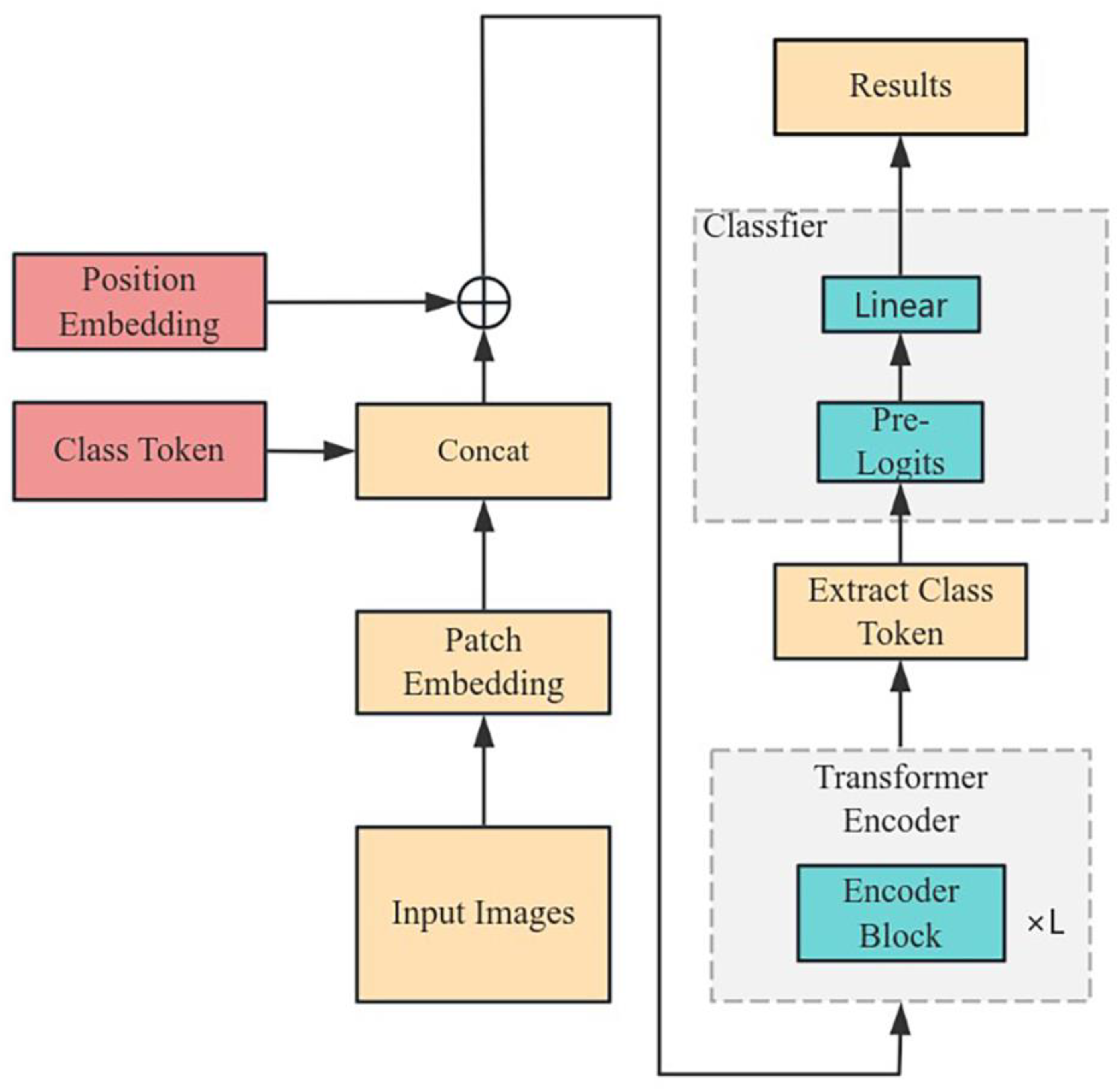
ViT is mainly composed of an embedding layer, an encoder (composed of Encoder Blocks), and a classifier, and its structure is shown in Figure 1.
The role of the embedding layer is to process the input images into the tokens required by the Transformer model. For the input image , where , , and are the height, width, and number of channels of the image, respectively, the image is first divided into patches of , and then each patch is linearly mapped to a one-dimensional vector, resulting in a token of length . In this paper, this part was implemented by a convolutional layer, which directly applied a convolutional kernel of size , stride , and number of kernels to the input image. The output of the convolutional layer is .
Then, a special category label was inserted into , and the shape of the concatenated token was . In order to make full use of the location information, the ViT model introduced a learnable position encoding matrix . The sum of position coding information and feature vector space was used as input of the Transformer Encoder:
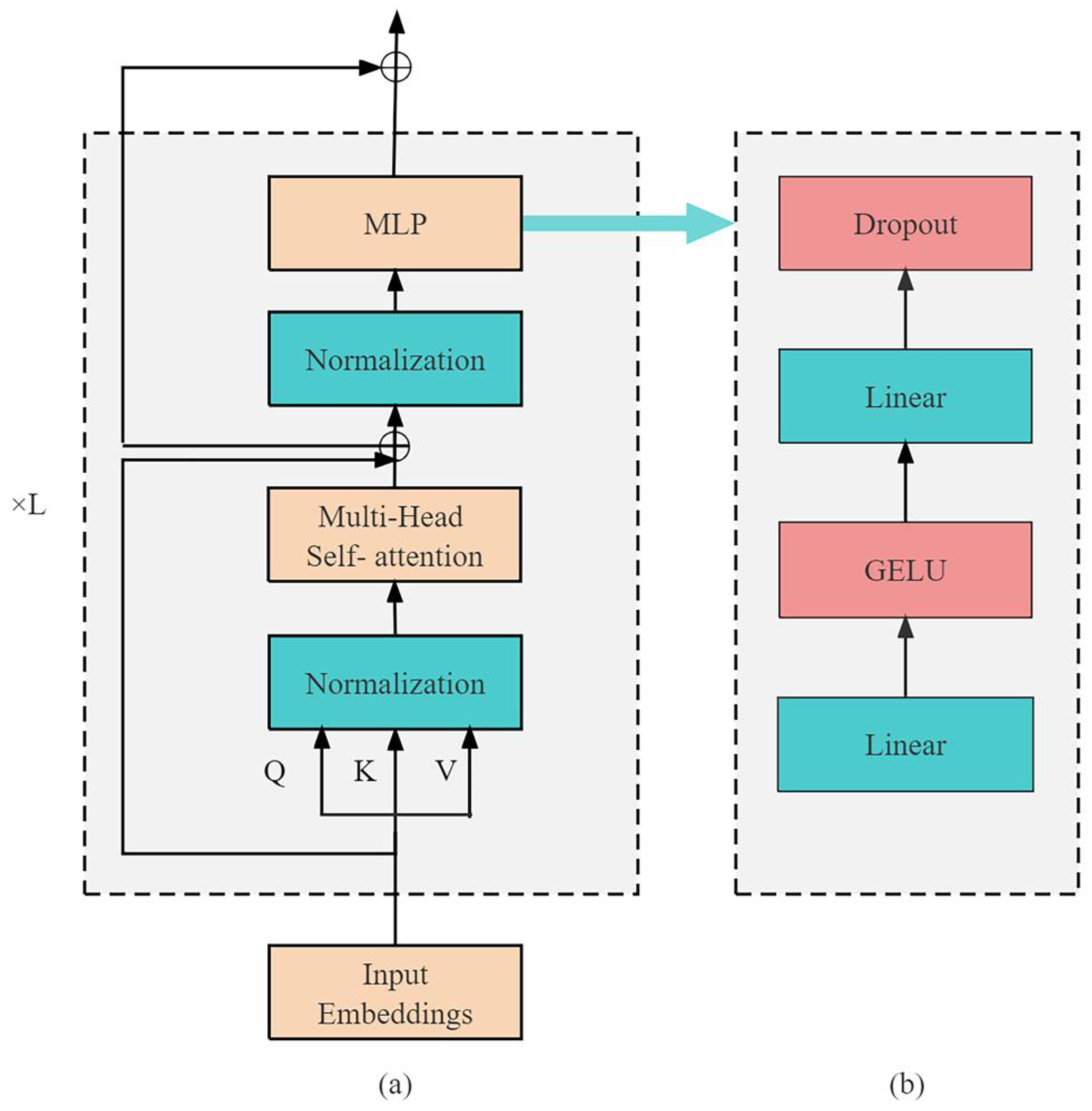
The Transformer encoder consists of identical stacked modules, and its internal structure is shown in Figure 2a. It mainly consists of two sub-layers, namely multi-head self-attention layer (MSA) and multilayer perception (MLP). Before data enters each sublayer, it was normalized using a normalization layer, and then fused by adding the output of each sublayer to the input of that sublayer. The encoder was set to layers, and the computation process of the l-th layer is as follows:
The encoding result after layers of encoder is .
ViT model adopts a multi-head self-attention mechanism, the multi-head self-attention layer uses multiple self-attention heads for parallel calculation, and finally splices the output of all self-attention heads together to get the result. The multilayer perception (MLP) is mainly composed of the fully connected layer, the GELU activation function, and the dropout layer, and its structure is shown in Figure 2b.
The classifier applies a nonlinear transformation to the encoder’s output and produces the final result of fault diagnosis.
2.4. Transfer Learning
Transfer learning is a machine learning technique that speeds up and improves the learning process by applying knowledge and model parameters gained from one task to another related task. Specifically, transfer learning leverages the knowledge learned from the source domain to assist learning in the target domain, aiming to enhance the model’s generalization performance in the target domain. Due to the fact that it is difficult to have bearing working in a faulty state for a long period of time in real operating conditions, the volume of bearing fault data samples in actual operating conditions is relatively small, which is quite different from the 14 million data samples in ImageNet-21k. Indeed, ViT models, like many other deep learning models, tend to rely on a larger amount of training data to achieve better performance. When the dataset is limited in size, it can be challenging to train a ViT model that exhibits optimal performance. To address this issue, this paper introduced a pre-trained ViT model trained on the ImageNet-21k dataset as the source model, and then the pre-trained model already was capable of extracting deep image features. Subsequently, a new model was created to be identical to the source model except for the output, which is changed to match the number of bearing fault categories in the target model. Finally, the target model was trained by inputting two-dimensional images generated from bearing vibration signals. The fine-tuned ViT transfer learning model can significantly reduce the training cost, improve the model’s generalization ability when the dataset is relatively small, and lower the required data cost.
3. Fault Diagnosis Experiment and Analysis
3.1. Dataset
The rolling bearing dataset used in this paper was derived from the Case Western Reserve University (CWRU) rolling bearing dataset [33]. An accelerometer sensor was used to collect the vibration acceleration signals of the bearing, which was installed near the bearing housing on the motor drive end, with a sampling frequency of 12 kHz. According to the different faulty parts, the bearing status is divided into four categories: rolling element fault, inner race fault, outer race fault, and normal operation state. The faulty bearing was installed in the test motor and makes the motor work under different loads, and the vibration data under different motor loads was recorded. The faulty signals collected in this paper were obtained from the driving end deep groove ball bearing SKF6205 under three different operating conditions with motor loads of 1~3 HP. Different motor loads correspond to different motor speeds, and the corresponding relationship between motor loads and motor speeds is shown in Table 1. The signals were collected in the form of acceleration data, sampled at a frequency of 12 kHz. The failure mode of the bearing was pitting corrosion.
3.2. Experimental Data Preparation
In this paper, the sliding time window method was used to perform overlapping sampling on the original vibration signals to reduce the risk of overfitting in the model.
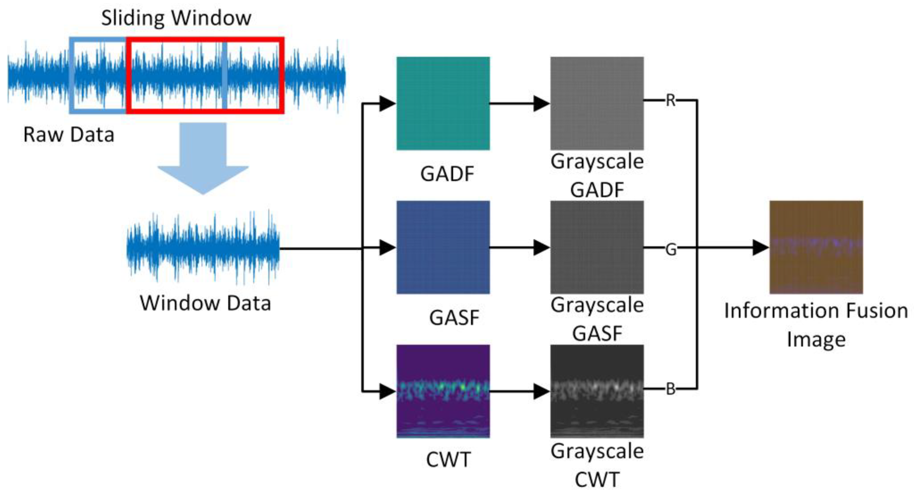
The accuracy of the model will increase with the increase of time window length, but a long time window length will make the calculation more complex and have little impact on the improvement of accuracy. Currently, the commonly used time window length is 1024, and this length had been proven to be a suitable time window length [36,37]. According to reference [25,38], the optimal input image size for the TLVIT model is 224 × 224. Therefore, in order to ensure that the pre-trained position encoding can continue to be used, this paper set the input image size of the model to 224 × 224. According to the calculation method of GAF, when the sliding time window length is 1120, the size of the generated GAF image is 1120 × 1120, which is exactly an integer multiple of the input image size selected in this article. Therefore, while ensuring the accuracy of the model, in order to facilitate the compression of image size by using the Python programming language, this article ultimately chose 1120 as the length of the time window. The sliding window length selected in the reference literature is 1024, with a sliding step size of 341 [37]. In this paper, the sliding step size is adjusted to 350 accordingly, referencing its window overlap rate. As shown in Figure 3, the blue box indicates the nth data sample, while the red box represents the (n+1)th data sample.
To ensure consistency in the number of channels for the ViT model, the sampled data were processed by using GASF, GADF, and CWT. These methods generated three pseudo-color images, which can be used as a control group in the study. The three pseudo-color images were converted to grayscale images, and an IFI was created by concatenating these grayscale feature images in the order of the RGB channels. It is as shown in Figure 3.
3.3. Fault Diagnosis Process
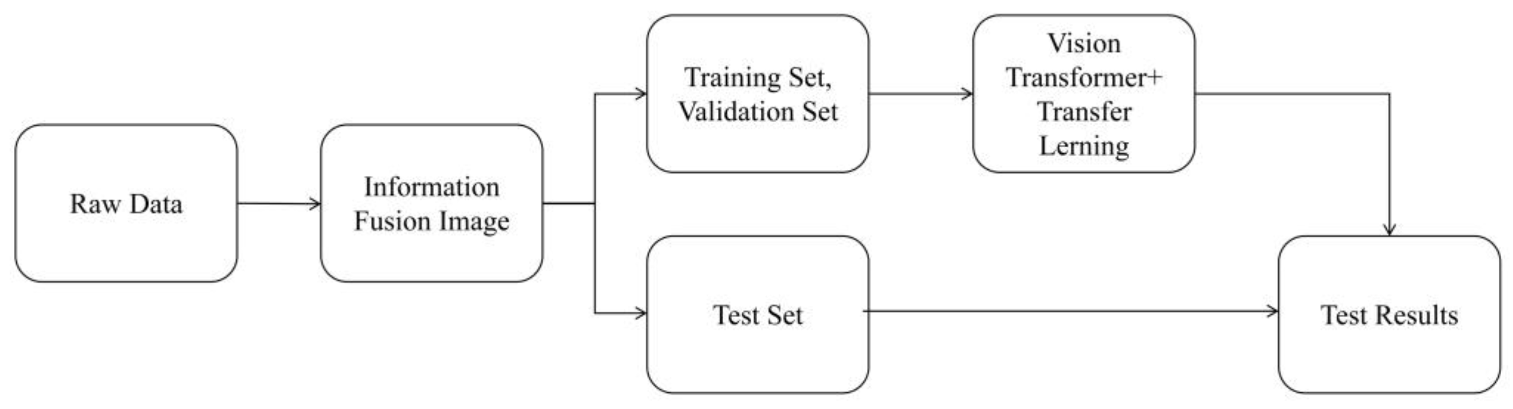
Figure 4 illustrates the fault diagnosis process by using the TLViT + IFI model. It involves converting the one-dimensional vibration signal into an IFI, partitioning the data into training, validation, and testing sets as required, training the ViT model by using transfer learning, and inputting the data samples from the test set into the trained TLViT model to obtain diagnosis results.
3.4. Model Training
The experiments described in the paper were implemented by using the TensorFlow 2.0 deep learning framework. TensorFlow 2.0 is a machine learning and deep learning framework developed by Google (Mountain View, CA, USA). It makes the development and deployment of machine learning models easier, more efficient, and more intuitive [39]. The data processing process in this paper was carried out on the Intel Core i7-12700H processor (manufactured by Intel Corporation in Santa Clara, CA, USA), and the model training process was carried out on the RTX3060 graphics card (manufactured by NVIDIA Corporation in Santa Clara, CA, USA). The Python version used was 3.8. In the experiment, firstly, data with motor loads of 1–3 HP were selected, and IFIs were generated form these three one-dimensional datasets by using the aforementioned method; then, three different two-dimensional image datasets, A, B, and C were obtained, each dataset containing 1600 samples with an equal number of samples for each fault category. The dataset was randomly partitioned into training, validation, and testing sets in a 6:2:2 ratios. To ensure the reproducibility of the partitioning results, a random seed was used to record the random partitioning process. The ViT model based on transfer learning (TLViT) was then fine-tuned and tested on the partitioned datasets separately. To avoid the influence of randomness in the experimental results, the experiment was repeated five times. Each time, a different random seed was used. The average accuracy on the testing set over the five repetitions was taken as the final result. To validate the performance of the TLViT model, a performance comparison experiment was conducted between different models. ResNet50 and ViT were used as the benchmark models, and they were trained and tested by using IFIs. In order to validate the effectiveness of the image fusion methods used, TLViT + CWT, TLViT + GASF, and TLViT + GADF were used as control experiments. In this study, all experiments were performed more than five times, and the average of the test results was taken as the final result. Based on previous experience, the training process of the ViT model typically stabilized after around 15 epochs. To balance the time cost of experiments and the stability of final training results, all experiments in this paper were set to run for 30 epochs with a batch size of 4. The stochastic gradient descent (SGD) optimization algorithm was selected [40], and during the training process, the weights of the model were recorded as the best weights when the validation loss is the lowest. These best weights were then used for testing on the testing set.
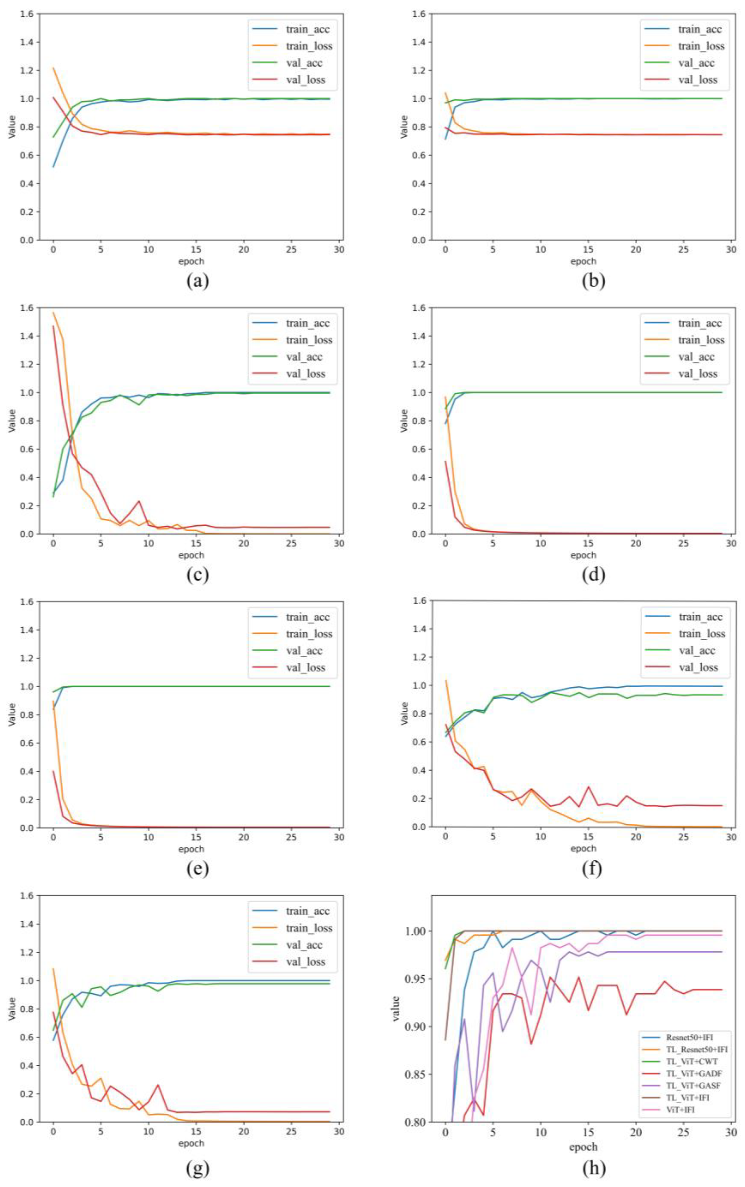
To observe the training process of each model more clearly, taking one training process of a model on dataset A as an example, the variation of the model’s loss and accuracy during training is shown in Figure 5. Figure 5h shows the comparison curve of the change of diagnosis accuracy of each model on the verification set during this training process, and the performance of each model can be preliminarily seen from the figure. To accurately evaluate the performance of each method, Table 2 provides the average accuracy on the testing set after five rounds of training and testing for each method on datasets A, B, and C. In the model performance comparison experiment, the ViT + IFI method achieved an accuracy of only 99.12% on the testing set. The performance of ResNet50 + IFI surpasses that of ViT + IFI, with an accuracy of 99.72% on testing set. This indicates that the performance of the ViT model cannot be fully utilized without pre-training on large datasets. As shown in Figure 5c,d, the TLResnet50 + IFI and TLViT + IFI models have high diagnosis accuracy at the beginning of training, indicating that the pre-trained models already have a certain fault diagnosis capability. The fact that both models ultimately achieved 100% diagnosis accuracy on the testing set demonstrates the effectiveness of transfer learning. This also indicates that it is difficult to compare the performance of the two models when there is an ample amount of training data in the target domain.
To verify the effectiveness of the proposed IFI, the TLViT model was trained and tested on pseudo-color image datasets generated using GADF, GASF, and CWT methods, respectively. The reason for using false color images is that the ViT model is greatly affected by the number of input image channels, so the three-channel image input is uniformly used in the controlled experiment. The TLViT + CWT model also achieved 100% diagnosis accuracy on the testing set, while the TLViT + GADF and TLViT + GASF performed less effectively, with accuracies of only 99.30% and 98.70% on the testing set, respectively. This indicates that using different methods to generate two-dimensional images from one-dimensional vibration signals results in varying diagnosis performance of the models. This difference in performance led to TLViT + GASF performing worse than ViT + IFI, highlighting the superiority of the proposed IFI.
3.5. Experimental Analysis of Small Samples
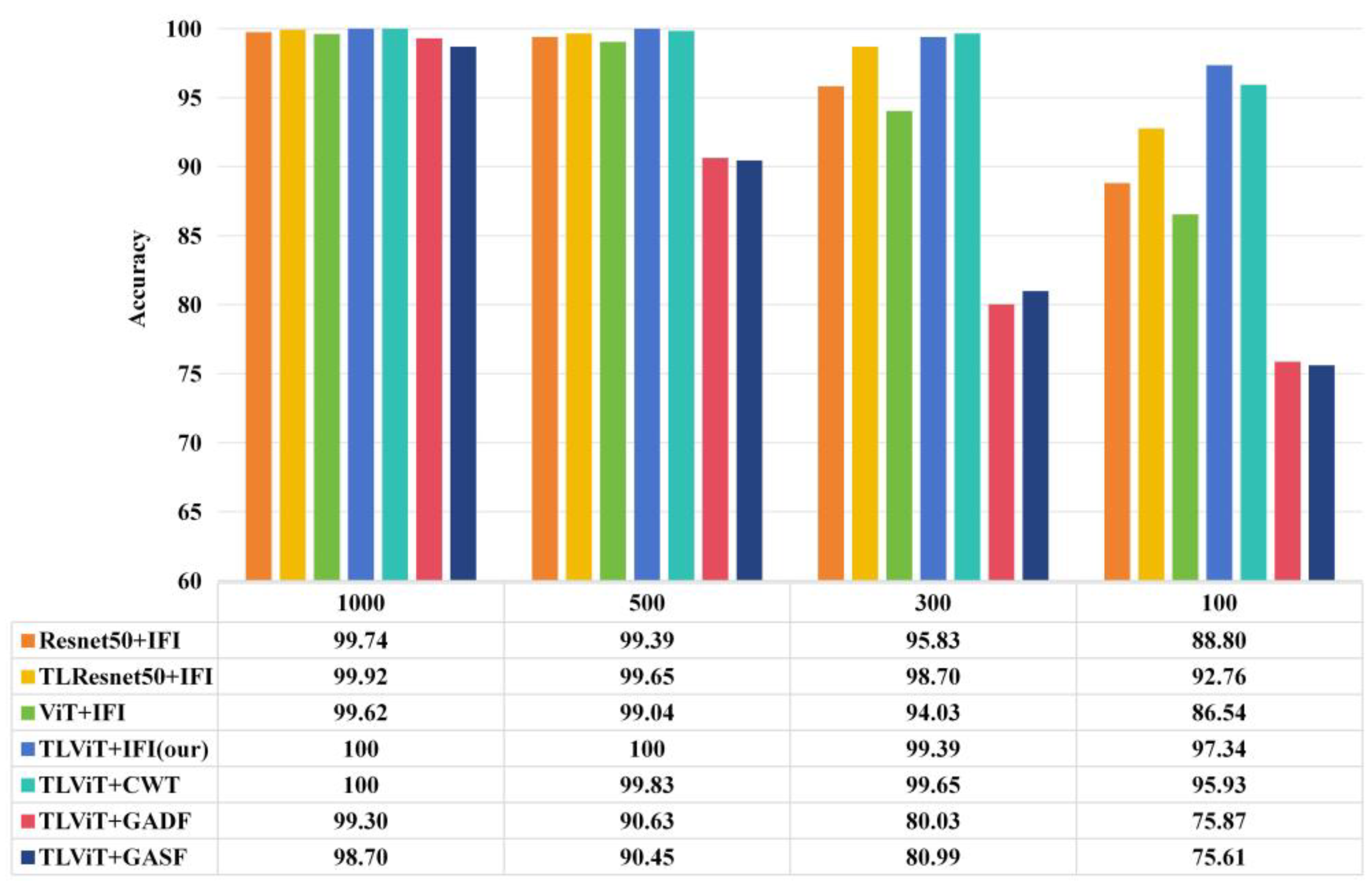
In practical working conditions, acquiring a substantial amount of fault data often poses challenges. Hence, it is imperative to ensure that fault diagnosis methods proposed under limited training data can uphold a commendable level of diagnostic accuracy. In this experiment, only the data with a motor load of 1HP were utilized to train the model by using four datasets comprising varying numbers of training samples. The dataset sizes were 1000, 500, 300, and 100, respectively, while each dataset consisted of 1152 test data samples. It is noteworthy that an equal number of training and test samples were allocated for each fault class within every dataset.
In the model performance comparison experiment, As shown in Figure 6, when the training sample is 1000, each method can achieve higher accuracy. With the decrease of training sample size, the fault diagnosis accuracy of all methods decreased, among which ViT + IFI model is the most affected, only 86.54% when the training sample size is 100, and the fault diagnosis ability decreased significantly. With the same number of training samples, the fault diagnosis accuracy of the Resnet50 + IFI model is slightly higher than that of the ViT + IFI model, and the diagnosis accuracy reaches 88.80% when the training sample size is 100, indicating that the ViT model without pre-training of large data sets has no advantage in diagnosis accuracy compared with the Resnet50 model.
The TLViT model based on transfer learning solves this problem. As shown in Figure 6, when the number of training samples in the target domain is 1000, 500, and 300, the diagnosis accuracy of TLViT model on the test set is slightly higher than that of TLResnet50 model, but there is no obvious difference between them. When there are 100 training samples in the target domain, TLViT can achieve 97.34% fault diagnosis accuracy on test set, while TLResnet50 + IFI diagnosis accuracy is only 92.76%, indicating that after pre-training on the same large data set, the fault diagnosis accuracy of TLresnet50 + IFI is only 92.76%. The performance of ViT model in this bearing fault diagnosis task exceeds that of Resnet50, which is more suitable for the case of less fault samples in the target domain. In the experiment to test the impact of image data generation on fault diagnosis methods, the fault diagnosis accuracy of each model gradually decreases with the reduction of the training sample size. Among them, TLViT + GADF and TLViT + GASF are most affected by the reduction of training sample size. When there are only 100 training data, the diagnosis accuracy on test set is only 75.87% and 75.61%. When the original data are small, it is not effective to convert one-dimensional vibration data into GAF images to train the model. Compared with TLViT + GADF and TLViT + GASF, TLViT + CWT has obvious advantages. When the amount of training data are only 100, the fault diagnosis accuracy on test set can reach 95.63%, but it is still lower than the 97.34% of TLViT + IFI. It shows that the IFI proposed in this paper can reduce the requirement of training data. It can be seen that TLViT + IFI model has strong diagnosis ability in the case of small samples.
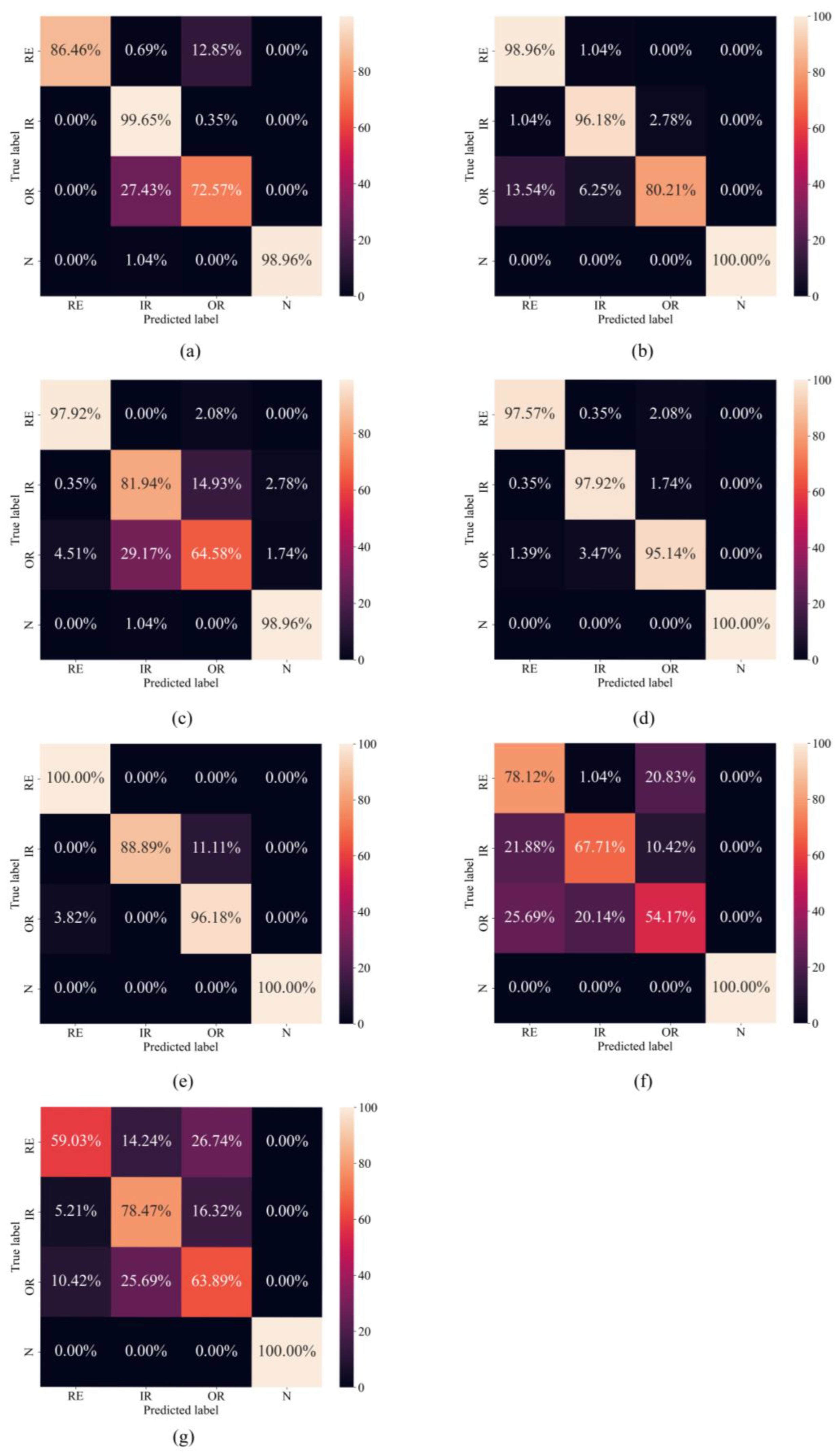
In order to more intuitively observe the fault diagnosis ability of the proposed methods under small sample conditions and the diagnosis of various kinds of faults, the test results of a training when the number of training samples of each method was 100 were visualized, and the confusion matrix was drawn. The X and Y axes in Figure 7 represent the predicted and actual categories, respectively.
3.6. Experimental Analysis of Variable Motor Load
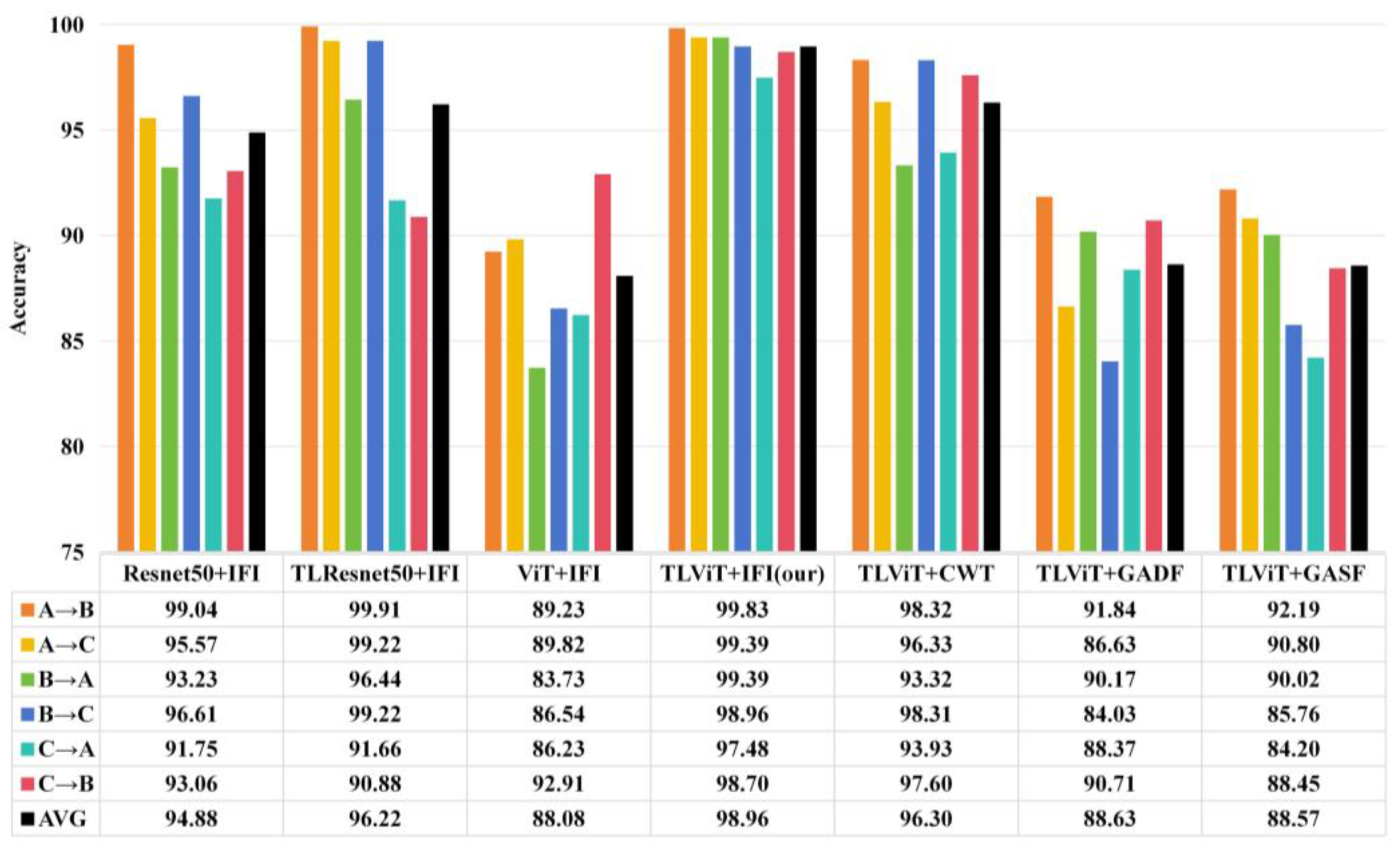
As can be seen from Table 2, each model has achieved high diagnosis accuracy under constant load. However, in the actual work process, the load of the motor often changes; this means that the speed of the bearing changes, so it is very important that the model can still be effectively diagnosed under the condition of variable motor load. In order to test the performance of the model proposed in this paper under varying loads, three datasets A, B, and C (corresponding to three loads of 1HP, 2HP, and 3HP, respectively), were used for training and testing. As shown in Figure 8, A→B means that A is used as the training set and B is used as the test set, and the same is true for other cases. AVG represents the average accuracy of the model under these variable conditions.
As can be seen from Figure 8, the average diagnosis accuracy of ViT + IFI model under variable load conditions is only 88.08%, lower than the average diagnosis accuracy of Resnet50 + IFI of 94.88%. The advantages of the ViT model have not been reflected, but the performance of the TLViT + IFI model, which uses a large amount of data for pre-training, has been significantly improved, and the average diagnosis accuracy under variable load conditions has reached 98.96%, which is more than 10% higher than that of ViT + IFI. The average diagnosis accuracy of TLResnet50 + IFI is 96.22%, indicating that TLViT model also has better performance under variable load conditions than TLResnet50. The average diagnosis accuracy of TLViT + GASF, TLViT + GADF, and TLViT + CWT models by using only one image as model input was 88.57%, 88.63%, and 96.30%, respectively. Moreover, the difference between the highest accuracy and the lowest accuracy is 7.99%, 7.81%, and 5%, respectively, while the average diagnosis accuracy of the TLViT + IFI method used in our study is 98.96%, and the difference between the highest accuracy and the lowest accuracy is 2.35%, indicating that the proposed method had higher diagnosis accuracy and better generalization.
3.7. Experimental Analysis of Anti-Noise Ability
In previous experiments, the TLViT + IFI method performed slightly better than TLViT + CWT method under small sample training and variable load conditions, but the gap between the two is not obvious. The anti-noise capability of the proposed method was further tested. This experiment was only to verify the noise resistance of the model, so only the samples in dataset A were used for training, and white Gaussian noise with different signal-to-noise ratios (SNRs) was added to the original data corresponding to dataset A, and then the data added with noise was converted into images, respectively, as the data of the test set. The SNR is defined as follows
where is the power of the original signal and is the power of the noise. From this formula, it can be seen that the SNR is inversely proportional to . The smaller the SNR is, the more serious the pollution in the original signal is.
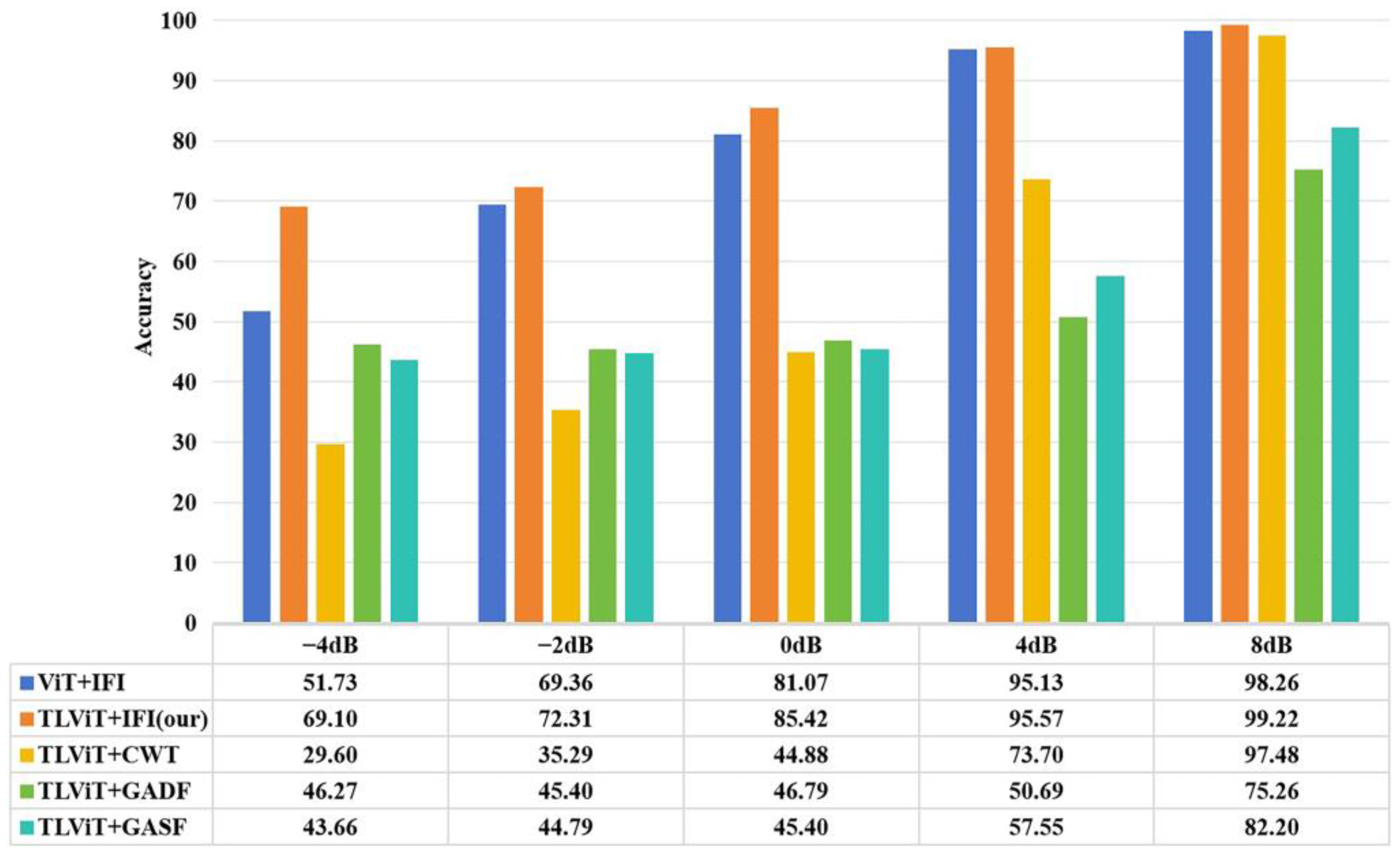
In order to verify that the IFI used in this paper has better noise resistance, only the TLViT model was used in the noise resistance comparison experiment. Figure 9 shows the results of TLViT model training on different image datasets and then testing under different SNR. It can be seen from the test results that images containing only one kind of image information have poor noise resistance. Under the influence of noise with a SNR of −4dB, the TLViT model is difficult to diagnose fault images containing only one kind of image information. The diagnosis accuracy of TLViT + CWT, TLViT + GASF, and TLViT + GADF are 29.60%, 46.27%, and 43.66%, respectively, and almost all lost the fault diagnosis capability. However, the TL_VIT + IFI proposed in this article still has a diagnosis accuracy of 69.10%, and the diagnosis accuracy is as high as 99.22% when the SNR is 8dB. It can be seen that the proposed image information fusion method greatly improves the anti-noise capability of the fault diagnosis model, because the fusion of multiple image information makes IFI have richer features and is not susceptible to noise.
4. Conclusions
A TLViT + IFI fault diagnosis method based on image information fusion was proposed to solve the problem of variable load conditions, less dataset, and noise in the working environment. The original signal was transformed into a grayscale image by using CWT, GASF, and GADF. This fused image effectively represented the signal characteristics in a comprehensive manner. Subsequently, the obtained IFI was input into the ViT for fault diagnosis based on transfer learning training. Consequently, the following conclusions can be derived.
In the model performance comparison experiment, the TLViT model trained based on transfer learning outperformed TLResnet50 under varying loads and small samples. When the number of training samples is 100, the fault diagnosis accuracy on the test set is 97.34%, indicating that this method can be applied to the situation with few training samples. The proposed method has an average diagnosis accuracy of 98.96% in the variable load condition, which is higher than other models, indicating that the fault diagnosis model trained by this method has good generalization.
The proposed IFI is more effective than the single image coding method. The test results of anti-noise performance show that when the SNR is −4 dB, the TLViT model is difficult to accurately diagnose the faults in the images generated by the control group method. However, the TLViT + IFI method can achieve a diagnosis accuracy of 69.10% on test set. It can be seen that IFI has higher anti-noise ability than the pseudo-color images generated using CWT, GADF, and GASF.
The above results show that the proposed TLViT + IFI fault diagnosis method has strong generalization and robustness under variable load, small sample, and noise environment, and can provide an effective idea for the research of rolling bearing fault diagnosis. Theoretically, this method can be used to diagnose the fault information in various time series forms, but only the vibration signal of the bearing, namely the acceleration sensor data, is discussed in this paper. In this paper, only the CWRU dataset was used for training and verification, and the bearing types and working conditions in the dataset were limited. In the process of converting time series data into IFIs, three methods, GASF, GADF, and CWT, need to be used first to generate grayscale maps, which increases the calculation cost. To solve the above problems, the author will carry out the following work in the follow-up research. (1) Explore the effect of combining other types of sensor data (such as temperature and sound signals) with the method proposed in this paper. (2) Validate the proposed method in more realistic and complex work environments. (3) The parameter volume of the Resnet50 model is 25.6 M [41], while the parameter volume of the ViT model used in this paper is 86M [25]; therefore, the lightweight treatment of the ViT model will be carried out in subsequent research, and the goal is to reduce its parameter volume by 50%.
Author Contributions
Z.Z.: Methodology, Formal analysis, Software, Validation and Writing—original draft. J.L.: Funding acquisition, Project administration, Formal analysis and Validation. C.C.: Funding acquisition, Methodology, Project administration, and Writing—review and editing. J.R.: Methodology, Formal analysis, Investigation and Writing—review and editing, Y.X.: Formal analysis, Investigation, and Writing—original draft. All authors have read and agreed to the published version of the manuscript.
Funding
This work was supported by the Hebei Nature Science Foundation under grant no. E2024402079, and Key Laboratory of Intelligent Industrial Equipment Technology of Hebei Province (Hebei University of Engineering) under grant no. 202206.
Institutional Review Board Statement
Not applicable.
Informed Consent Statement
Not applicable.
Data Availability Statement
The data were collected from a publicly available CWRU bearing database. The link is as follows: https://engineering.case.edu/bearingdatacenter/download-data-file (accessed on 20 March 2024).
Conflicts of Interest
The authors declare no conflicts of interests.
References
- Rai, A.; Upadhyay, S.H. A Review on Signal Processing Techniques Utilized in the Fault Diagnosis of Rolling Element Bearings. Tribol. Int. 2016, 96, 289–306. [Google Scholar] [CrossRef]
- Zhang, S.; Zhang, S.; Wang, B.; Habetler, T.G. Deep Learning Algorithms for Bearing Fault Diagnostics—A Comprehensive Review. IEEE Access 2020, 8, 29857–29881. [Google Scholar] [CrossRef]
- Song, W.; Xiang, J. A Method Using Numerical Simulation and Support Vector Machine to Detect Faults in Bearings. In Proceedings of the 2017 International Conference on Sensing, Diagnostics, Prognostics, and Control (SDPC), Shanghai, China, 16–18 August 2017; pp. 603–607. [Google Scholar]
- Zhu, H.; Li, X.; Liu, H. Fault Diagnosis of Rolling Bearing Based on WT-VMD and Random Forest. In Proceedings of the 2020 Chinese Control And Decision Conference (CCDC), Hefei, China, 22–24 August 2020; pp. 2130–2135. [Google Scholar]
- Amarnath, M.; Sugumaran, V.; Kumar, H. Exploiting Sound Signals for Fault Diagnosis of Bearings Using Decision Tree. Measurement 2013, 46, 1250–1256. [Google Scholar] [CrossRef]
- Fuan, W.; Hongkai, J.; Haidong, S.; Wenjing, D.; Shuaipeng, W. An Adaptive Deep Convolutional Neural Network for Rolling Bearing Fault Diagnosis. Meas. Sci. Technol. 2017, 28, 095005. [Google Scholar] [CrossRef]
- Eren, L.; Ince, T.; Kiranyaz, S. A Generic Intelligent Bearing Fault Diagnosis System Using Compact Adaptive 1D CNN Classifier. J. Signal Process. Syst. 2019, 91, 179–189. [Google Scholar] [CrossRef]
- Song, X.; Cong, Y.; Song, Y.; Chen, Y.; Liang, P. A Bearing Fault Diagnosis Model Based on CNN with Wide Convolution Kernels. J. Ambient Intell. Humaniz. Comput. 2022, 13, 4041–4056. [Google Scholar] [CrossRef]
- Guo, Y.; Zhou, Y.; Zhang, Z. Fault Diagnosis of Multi-Channel Data by the CNN with the Multilinear Principal Component Analysis. Measurement 2021, 171, 108513. [Google Scholar] [CrossRef]
- Liu, X.; Centeno, J.; Alvarado, J.; Tan, L. One Dimensional Convolutional Neural Networks Using Sparse Wavelet Decomposition for Bearing Fault Diagnosis. IEEE Access 2022, 10, 86998–87007. [Google Scholar] [CrossRef]
- Liu, H.; Zhou, J.; Zheng, Y.; Jiang, W.; Zhang, Y. Fault Diagnosis of Rolling Bearings with Recurrent Neural Network-Based Autoencoders. ISA Trans. 2018, 77, 167–178. [Google Scholar] [CrossRef]
- Zou, P.; Hou, B.; Lei, J.; Zhang, Z. Bearing Fault Diagnosis Method Based on EEMD and LSTM. Int. J. Comput. Commun. Control 2020, 15. [Google Scholar] [CrossRef]
- Pan, H.; He, X.; Tang, S.; Meng, F. An Improved Bearing Fault Diagnosis Method using One-Dimensional CNN and LSTM. J. Mech. Eng. 2018, 64, 443. [Google Scholar]
- Hoang, D.-T.; Kang, H.-J. Convolutional Neural Network Based Bearing Fault Diagnosis. In Proceedings of the Intelligent Computing Theories and Application, Liverpool, UK, 7–10 August 2017; Huang, D.-S., Jo, K.-H., Figueroa-García, J.C., Eds.; Springer International Publishing: Cham, Switzerland, 2017; pp. 105–111. [Google Scholar]
- Zhou, F.; Zhou, W.; Chen, D.; Wen, C. Rolling Bearing Real Time Fault Diagnosis Using Convolutional Neural Network. In Proceedings of the 2019 Chinese Control And Decision Conference (CCDC), Nanchang, China, 3–5 June 2019; pp. 377–382. [Google Scholar]
- Wen, L.; Li, X.; Gao, L.; Zhang, Y. A New Convolutional Neural Network-Based Data-Driven Fault Diagnosis Method. IEEE Trans. Ind. Electron. 2018, 65, 5990–5998. [Google Scholar] [CrossRef]
- Luo, H.; Bo, L.; Peng, C.; Hou, D. An Improved Convolutional-Neural-Network-Based Fault Diagnosis Method for the Rotor–Journal Bearings System. Machines 2022, 10, 503. [Google Scholar] [CrossRef]
- Guo, Y.; Mao, J.; Zhao, M. Rolling Bearing Fault Diagnosis Method Based on Attention CNN and BiLSTM Network. Neural Process. Lett. 2023, 55, 3377–3410. [Google Scholar] [CrossRef]
- Yang, S.; Liu, Y.; Tian, X.; Ma, L. Bearing Fault Diagnosis Based on Attentional Multi-Scale CNN. In Proceedings of the Intelligent Robotics and Applications, Yantai, China, 22–25 October 2021; Liu, X.-J., Nie, Z., Yu, J., Xie, F., Song, R., Eds.; Springer International Publishing: Cham, Switzerland, 2021; pp. 25–36. [Google Scholar]
- Yuan, X.; Zhang, H.; Liu, H. A Novel Fault Diagnosis Approach for Rolling Bearing Based on CWT and Adaptive Sparse Representation. Shock Vib. 2022, 2022, e9079790. [Google Scholar] [CrossRef]
- Zhang, Q.; Deng, L. An Intelligent Fault Diagnosis Method of Rolling Bearings Based on Short-Time Fourier Transform and Convolutional Neural Network. J Fail. Anal. Preven. 2023, 23, 795–811. [Google Scholar] [CrossRef]
- Zhou, Y.; Long, X.; Sun, M.; Chen, Z. Bearing Fault Diagnosis Based on Gramian Angular Field and DenseNet. MBE 2022, 19, 14086–14101. [Google Scholar] [CrossRef]
- Sun, Y.; Wang, W. Role of Image Feature Enhancement in Intelligent Fault Diagnosis for Mechanical Equipment: A Review. Eng. Fail. Anal. 2024, 156, 107815. [Google Scholar] [CrossRef]
- Vaswani, A.; Shazeer, N.; Parmar, N.; Uszkoreit, J.; Jones, L.; Gomez, A.N.; Kaiser, Ł.; Polosukhin, I. Attention Is All You Need. In Proceedings of the Advances in Neural Information Processing Systems, Long Beach, CA, USA, 4–9 December 2017; Curran Associates, Inc.: San Francisco, CA, USA, 2017; Volume 30. [Google Scholar]
- Dosovitskiy, A.; Beyer, L.; Kolesnikov, A.; Weissenborn, D.; Zhai, X.; Unterthiner, T.; Dehghani, M.; Minderer, M.; Heigold, G.; Gelly, S.; et al. An Image Is Worth 16x16 Words: Transformers for Image Recognition at Scale. arXiv 2020, arXiv:2010.11929. [Google Scholar]
- Pan, S.J.; Yang, Q. A Survey on Transfer Learning. IEEE Trans. Knowl. Data Eng. 2010, 22, 1345–1359. [Google Scholar] [CrossRef]
- Ben-David, S.; Blitzer, J.; Crammer, K.; Kulesza, A.; Pereira, F.; Vaughan, J.W. A Theory of Learning from Different Domains. Mach Learn 2010, 79, 151–175. [Google Scholar] [CrossRef]
- Shao, S.; McAleer, S.; Yan, R.; Baldi, P. Highly Accurate Machine Fault Diagnosis Using Deep Transfer Learning. IEEE Trans. Ind. Inform. 2019, 15, 2446–2455. [Google Scholar] [CrossRef]
- Wang, Z.; He, X.; Yang, B.; Li, N. Subdomain Adaptation Transfer Learning Network for Fault Diagnosis of Roller Bearings. IEEE Trans. Ind. Electron. 2022, 69, 8430–8439. [Google Scholar] [CrossRef]
- Wang, R.; Huang, W.; Wang, J.; Shen, C.; Zhu, Z. Multisource Domain Feature Adaptation Network for Bearing Fault Diagnosis Under Time-Varying Working Conditions. IEEE Trans. Instrum. Meas. 2022, 71, 3511010. [Google Scholar] [CrossRef]
- He, J.; Ouyang, M.; Chen, Z.; Chen, D.; Liu, S. A Deep Transfer Learning Fault Diagnosis Method Based on WGAN and Minimum Singular Value for Non-Homologous Bearing. IEEE Trans. Instrum. Meas. 2022, 71, 3509109. [Google Scholar] [CrossRef]
- Jiang, L.; Zheng, C.; Li, Y. Rotating Machinery Fault Diagnosis Based on Transfer Learning and an Improved Convolutional Neural Network. Meas. Sci. Technol. 2022, 33, 105012. [Google Scholar] [CrossRef]
- Bearing Data Center|Case School of Engineering|Case Western Reserve University. Available online: https://engineering.case.edu/bearingdatacenter (accessed on 20 March 2024).
- Lin, J.; Qu, L. Feature extraction based on Morlet wavelet and its application for mechanical fault diagnosis. J. Sound Vib. 2000, 234, 135–148. [Google Scholar] [CrossRef]
- Tang, B.; Liu, W.; Song, T. Wind Turbine Fault Diagnosis Based on Morlet Wavelet Transformation and Wigner-Ville Distribution. Renew. Energy 2010, 35, 2862–2866. [Google Scholar] [CrossRef]
- Xu, Z.; Tang, X.; Wang, Z. A Multi-Information Fusion ViT Model and Its Application to the Fault Diagnosis of Bearing with Small Data Samples. Machines 2023, 11, 277. [Google Scholar] [CrossRef]
- Cai, C.; Li, R.; Ma, Q.; Gao, H. Bearing Fault Diagnosis Method Based on the Gramian Angular Field and an SE-ResNeXt50 Transfer Learning Model. Insight—Non-Destr. Test. Cond. Monit. 2023, 65, 695–704. [Google Scholar] [CrossRef]
- Deng, J.; Dong, W.; Socher, R.; Li, L.-J.; Kai, L.; Li, F.-F. ImageNet: A Large-Scale Hierarchical Image Database. In Proceedings of the 2009 IEEE Conference on Computer Vision and Pattern Recognition, Miami, FL, USA, 20–25 June 2009; pp. 248–255. [Google Scholar]
- Introduction to TensorFlow. Available online: https://tensorflow.google.cn/learn (accessed on 20 March 2024).
- Bottou, L. Large-Scale Machine Learning with Stochastic Gradient Descent. In Proceedings of the COMPSTAT’2010: 19th International Conference on Computational Statistics, Paris, France, 22–27 August 2010; pp. 177–186, ISBN 978-3-7908-2604-3. [Google Scholar]
- He, K.; Zhang, X.; Ren, S.; Sun, J. Deep Residual Learning for Image Recognition. In Proceedings of the 2016 IEEE Conference on Computer Vision and Pattern Recognition (CVPR), Las Vegas, NV, USA, 27–30 June 2016; pp. 770–778. [Google Scholar]
Figure 1.
The structure of Vision Transformer.

Figure 2.
Transformer Encoder. (a) Encoder block. (b) MLP block.

Figure 3.
The process of converting time series data to IFI.

Figure 4.
Fault diagnosis process of the TLViT + IFI.

Figure 5.
Accuracy and loss of training set and validation set during training. (a) ViT + IFI, (b) Resnet50 + IFI, (c) TLViT + IFI, (d) TLResnet50 + IFI, (e) TLViT + CWT, (f) TLViT + GADF, (g) TLViT + GASF, and (h). Comparison of accuracy changes of each model on validation set.
Figure 5.
Accuracy and loss of training set and validation set during training. (a) ViT + IFI, (b) Resnet50 + IFI, (c) TLViT + IFI, (d) TLResnet50 + IFI, (e) TLViT + CWT, (f) TLViT + GADF, (g) TLViT + GASF, and (h). Comparison of accuracy changes of each model on validation set.

Figure 6.
Diagnosis accuracy under different number of training samples.

Figure 7.
Confusion matrix of test results. (a) Resnet50 + IFI, (b) TLResnet50 + IFI, (c) ViT + IFI, (d) TLViT + IFI, (e) TLViT + CWT, (f) TLViT + GADF, and (g) TLViT + GASF.
Figure 7.
Confusion matrix of test results. (a) Resnet50 + IFI, (b) TLResnet50 + IFI, (c) ViT + IFI, (d) TLViT + IFI, (e) TLViT + CWT, (f) TLViT + GADF, and (g) TLViT + GASF.

Figure 8.
The diagnosis accuracy of each method under variable load condition.

Figure 9.
The diagnosis accuracy of each method under different SNR.


Table 1.
Motor loads and motor speeds.
| Motor Load (HP) | Motor Speed (RPM) |
|---|---|
| 1 | 1772 |
| 2 | 1750 |
| 3 | 1730 |
Table 2.
Average accuracy on test set.
| Fault Diagnosis Method | Average Accuracy on the Test Set |
|---|---|
| Resnet50 + IFI | 99.72% |
| TLResnet50 + IFI | 100% |
| ViT + IFI | 99.12% |
| TLViT + IFI | 100% |
| TLViT + CWT | 100% |
| TLViT + GADF | 99.30% |
| TLViT + GASF | 98.70% |
Disclaimer/Publisher’s Note: The statements, opinions and data contained in all publications are solely those of the individual author(s) and contributor(s) and not of MDPI and/or the editor(s). MDPI and/or the editor(s) disclaim responsibility for any injury to people or property resulting from any ideas, methods, instructions or products referred to in the content. |
© 2024 by the authors. Licensee MDPI, Basel, Switzerland. This article is an open access article distributed under the terms and conditions of the Creative Commons Attribution (CC BY) license (https://creativecommons.org/licenses/by/4.0/).
Share and Cite
MDPI and ACS Style
Zhang, Z.; Li, J.; Cai, C.; Ren, J.; Xue, Y. Bearing Fault Diagnosis Based on Image Information Fusion and Vision Transformer Transfer Learning Model. Appl. Sci. 2024, 14, 2706. https://0-doi-org.brum.beds.ac.uk/10.3390/app14072706
AMA Style
Zhang Z, Li J, Cai C, Ren J, Xue Y. Bearing Fault Diagnosis Based on Image Information Fusion and Vision Transformer Transfer Learning Model. Applied Sciences. 2024; 14(7):2706. https://0-doi-org.brum.beds.ac.uk/10.3390/app14072706
Chicago/Turabian StyleZhang, Zichen, Jing Li, Chaozhi Cai, Jianhua Ren, and Yingfang Xue. 2024. "Bearing Fault Diagnosis Based on Image Information Fusion and Vision Transformer Transfer Learning Model" Applied Sciences 14, no. 7: 2706. https://0-doi-org.brum.beds.ac.uk/10.3390/app14072706
Note that from the first issue of 2016, this journal uses article numbers instead of page numbers. See further details here.