Two-Polarisation Physical Model of Bowed Strings with Nonlinear Contact and Friction Forces, and Application to Gesture-Based Sound Synthesis ^†

Abstract

Recent bowed string sound synthesis has relied on physical modelling techniques; the achievable realism and flexibility of gestural control are appealing, and the heavier computational cost becomes less significant as technology improves. A bowed string sound synthesis algorithm is designed, by simulating two-polarisation string motion, discretising the partial differential equations governing the string’s behaviour with the finite difference method. A globally energy balanced scheme is used, as a guarantee of numerical stability under highly nonlinear conditions. In one polarisation, a nonlinear contact model is used for the normal forces exerted by the dynamic bow hair, left hand fingers, and fingerboard. In the other polarisation, a force-velocity friction curve is used for the resulting tangential forces. The scheme update requires the solution of two nonlinear vector equations. The dynamic input parameters allow for simulating a wide range of gestures; some typical bow and left hand gestures are presented, along with synthetic sound and video demonstrations.

1. Introduction

Sound synthesis techniques for string instruments have evolved, in the past few decades, from abstract synthesis [1] (wavetables, frequency-modulation (FM) synthesis ...) towards sampling synthesis, based on a library of pre-recorded sounds, and physical models, emulating the instruments themselves. To this day, the best synthesised sound quality is achieved by sampling techniques; however, the potentially very large storage requirements for these sound libraries are a major argument for using physical models. Beyond the storage concerns, the use of a physical model allows for great flexibility for input parameters (typically, the instrument’s shape and material properties, together with the player’s controls), as well as output parameters, usually the “listening conditions”, that can be changed freely and dynamically along a simulation, as opposed to the case of statically recorded samples.

Physical modelling synthesis for strings debuted in the 1970s, with time stepping methods to discretise and directly solve the 1D wave equation [2,3,4]. However, the very limited computational power at the time ruled out simulation at an audio sample rate in any reasonable amount of time. The next generation of models therefore focussed on algorithmic simplification, through physically plausible assumptions. The physics-based Karplus-Strong string synthesis algorithm [5,6] was generalised by the digital waveguide framework [7,8]; Karjalainen et al. [9] review the use of these models for string synthesis. Their fast execution and realistic sound output found efficient applications in bowed string modelling, and are still widely used to this day [10,11,12,13,14]. Digital waveguides model the forward and backward travelling waves along a string using delay lines—a simple and efficient strategy for certain linear time invariant systems. In particular, they are well suited for systems in one dimension, well described by the wave equation. Another more general class of physical models relies on the modal solutions of the string equation, and has been successfully adapted for bowed strings [15,16].

However, the very assumptions that underlie the efficiency of these methods can lead to difficulties when extensions to more realistic settings are desired—the bowed string and its complex, nonlinear, time-varying interaction with the environment being an excellent example. Time-stepping methods, and more specifically finite difference methods [17], though computationally costly, have regained appeal in musical sound synthesis [18] with the great increase in computing power during the last two decades. String simulation in one dimension is particularly suited for these kind of methods [19,20]. The interactions of, say, a bowed string with its environment can be included in a straightforward manner, as long as they can be described with a system of partial differential equations (PDEs). These methods also allow a greater flexibility for modelling the musician’s gestures, and more generally to deal with the dynamic nature of the input and output parameters.

While the number of parameters is small compared to other methods, navigating the space they describe is somewhat of a challenge. Indeed, as opposed to a struck or plucked string, the continuous excitation mechanism of a bowed string makes playability a major issue, for real or virtual instruments. The player shapes the sound and behaviour of his instrument throughout the whole production of a note. Their gestures can be described with a handful of parameters, which must be perfectly coordinated at all times to allow a tone to be created and sustained; indeed, Schelleng [21], following the work of Raman [22] some decades earlier, was the first to analytically show that, under simplifying assumptions and for a certain bow velocity, only a relatively narrow triangular area (in logarithmic scale) in the downwards bow force versus bow-bridge distance parameter space gave rise to the characteristic stable Helmholtz motion desired by most musicians (his work was revised by Schoonderwaldt et al. [23], introducing more refined elements of bowed string motion). This area is tied to the concept of playability, and the so-called Schelleng diagrams are widely used in bowed string playability studies [24,25,26,27]. Transient quality also constitutes a major part of playability: Guettler [28] investigated the relation between bow downwards force and bow acceleration regarding the quality of initial transients, producing triangular diagrams resembling those of Schelleng, again under simplifying assumptions; Woodhouse et al. [29] produced Guettler diagrams with more refined numerical models as well as experimental data, showing the predicted wedge-shaped region. A detailed review of the published literature on bowed string mechanics (and, indeed, violin acoustics in general) was recently written by Woodhouse [30].

After the studies of Schelleng, an experimental study by Askenfelt [31,32] yielded measured values for these control parameters, on a violin; he was the first to develop a measuring rig able to record them all simultaneously during performance. More recently, the variation of these parameters along various bowed string gestures was observed and analysed in detail [15,33,34]. The obtained signals can be mathematically reconstructed [35], or directly used, to be fed into a physical modelling algorithm such as the one presented in this work. The aforementioned studies are mainly interested in bowing gestures; to handle those of the left hand fingers (vibrato, legato, glissando, etc.), one can include a finger model, along with a fingerboard.

This work is concerned with a detailed model of bowed string vibration, emphasising the interactions of the string with the player. A linear bowed string is simulated in two polarisations. The model includes the following features:

• in one polarisation, distributed nonlinear contact interactions between the string and the dynamic left hand fingers, dynamic bow, and fingerboard. A stable finite difference scheme for modelling distributed contact/collisions has recently been established [36,37], that can be used in this stopped string-fingerboard setup [38,39];
• in the other polarisation, orthogonally to the first, distributed nonlinear friction forces between the string and the same three objects. The friction force nonlinearity is modelled with a force/velocity friction curve for the bow [40]. Tangential Coulomb friction also keeps the string captured between the fingers and fingerboard during note production;
• full control over the physical parameters of the system, as well as dynamic variations of the playing parameters. This time domain model is therefore able to reproduce most bowed string gestures;
• introduction of an inertial term in the bow model, in the tangential direction. This leads to a horizontal force bow control, instead of the bow velocity input signal used in most of the aforementioned models;
• in the same direction, introduction of an inertial term and a restoring term in the finger model. The fingertip is massive, absorbs some of the tangential string vibrations, and oscillates about a fixed horizontal finger position.

The main challenges associated with this model are computational. On one hand, the resulting numerical method must be stable; energy methods are used to derive a stability condition from the model system, and establish a power balance to keep track of the energy exchanges between the various parts of the system. On the other hand, the distributed nonlinearities induce heavy computational costs, with the need to resort to iterative nonlinear system solving methods; extensive optimisation is necessary in order to bring the algorithm closer to real-time operation. Finally, the gestural control is obviously limited by the aforementioned playability issues; such a model is able to produce waveforms outside of the generally desired Helmholtz sawtooth, and the absence of direct feedback for the player in the present algorithm indeed makes parameter control a rather fastidious task.

In Section 2, the model equations for the bow/string system are presented, with an elaborate description of finger/string interaction in the case of stopped notes, and the string/fingerboard collision interaction. A globally energy balanced finite difference scheme is presented in Section 3. Finally, bowed string simulation results, with the reproduction of several typical gestures, are presented in Section 4. Some sound and video examples from the computed simulations are available online [41].

2. Model Description

2.1. Context

The choice of time-stepping methods is in line with the larger aim of building full physical models of musical instruments, embedded in virtual acoustic spaces. The work presented here is a step towards designing such a model for a bowed string instrument; this longer term aim guided the choice of whether or not to include certain features of bowed string playing in this work.

As a consequence, although the bowed string model described here uses sensible, physical assumptions, some of its features may not be as refined as one can find in some of the recent literature. This is the result of compromising between physical accuracy, computational complexity, and (subjective) synthetic sound quality. Some features, for instance, have been neglected for dramatically increasing the algorithmic complexity and computational load, while having very little influence to both the output sound and the control quality; this is the case for e.g., the nonlinear intrinsic coupling between the two polarisations of the string, or the thermal properties of the rosin layer coating the bow [42]. Torsion waves are also excluded; although, when present, their synchronisation with transverse waves has been experimentally shown to strongly contribute to tone quality and stability [43], their presence (or absence) may not have a strong bearing on the playability and synthetic sound quality of a simplified physical model [25].

2.2. A Linear, Two-Polarisation String Model

A dual-polarisation string model serves two main purposes in this work. First, treated in this paper, is the ability to simulate realistic, nonlinear impact interactions between the string and any external objects in one direction, translating directly into tangential friction forces in the other direction. This is an intuitive way to include not only a bow that is able to naturally bounce, but also dynamic left hand fingers to stop the string against a fingerboard, while absorbing some of the string vibrations.

Second is the potential to use this algorithm towards a model of a full instrument. The coupling of the two polarisations at the bridge boundary, through a model of the bridge itself coupled to the instrument body, would be straightforwardly achieved with this string model as a starting point. While the incorporation of the bridge and wooden cavity is undoubtedly crucial to the final sound of the virtual instrument, let us first describe the proposed string model.

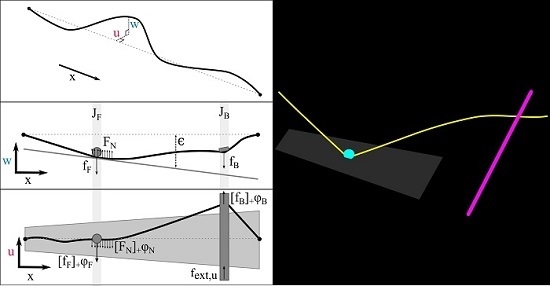
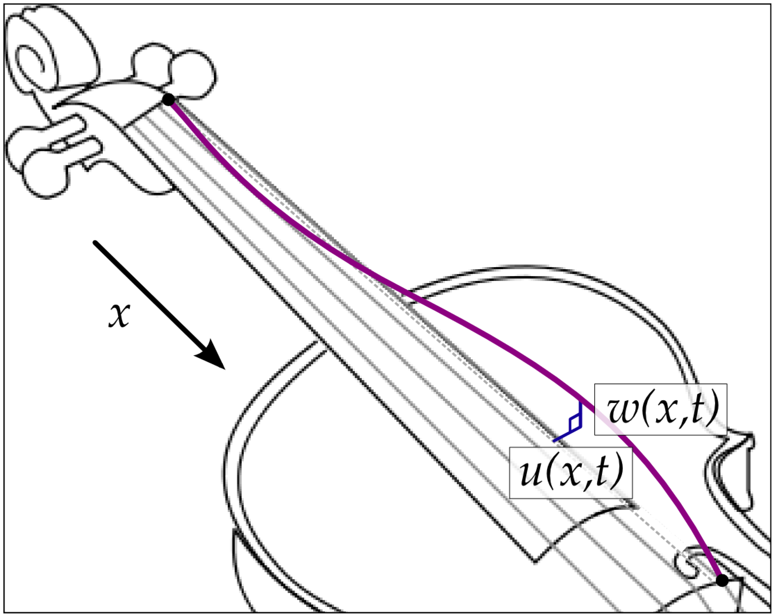
2.3. The Isolated String

Consider a linear, stiff, and lossy string, of length L. The string displacement in the vertical or normal polarisation is denoted by $w(x,t)$, while $u(x,t)$ is the string displacement in the horizontal or tangential polarisation. Both are defined for position $x\in \mathcal{D}=\left[0,L\right]$ and time $t\in {\mathbb{R}}^{+}=\left[0,+\infty \right]$ (see Figure 1).

The partial differential equations governing the time evolution of $u(x,t)$ and $w(x,t)$ can be written as:

$$\mathcal{L}w=0$$

(1a)

$$\mathcal{L}u=0$$

(1b)

$\mathcal{L}$ is the partial differential operator defined as [20]:

$$\mathcal{L}=\mathsf{\rho }{\partial }_t^2-T{\partial }_x^2+E{I}_0{\partial }_x^4+{\mathsf{\lambda }}_1\mathsf{\rho }{\partial }_t-{\mathsf{\lambda }}_2\mathsf{\rho }{\partial }_t{\partial }_x^2$$

(2)

where ${\partial }_{·}^i$ is equivalent to $\frac{{\partial }^i}{\partial {·}^i}$. $\mathsf{\rho }$ is the linear mass density of the string, in kg/m; T is the tension of the string, in N; $E{I}_0$ is the bending stiffness, where E is Young’s modulus in Pa, and $I_0=\frac{\pi r^4}{4}$ is the area moment of inertia of the circular cross-section of the string, with r the string radius in m. Some typical parameters for a violin, a viola, and a cello, can be found in the literature, notably those measured by Pickering [44] and Percival [45].

${\mathsf{\lambda }}_1$ (1/s) and ${\mathsf{\lambda }}_2$ (m²/s) are positive damping coefficients, that empirically account for frequency independent and dependent losses in the string, respectively. With more refinement, they could be replaced by a full model accounting for energy dissipation through air viscosity, acoustic radiation, and internal friction, each of these three mechanisms having a more or less pronounced impact across the spectrum [46]. In accordance with the statements in Section 2.1 however, this empirical, simplified loss model is deemed sufficient for the purposes of this work.

The system described by Equations (1) and (2) is accompanied by a set of boundary conditions (four of them for each polarisation of the stiff string). Standard energy conserving conditions of the simply supported type are chosen, assuming an isolated string, with no interaction with the instrument body (note that for the musical string, the effect of bending stiffness being very small with respect to that of tension, there is little difference between the simply supported and clamped boundary conditions):

$$\begin{array}{cc}\hfill w(0,t)& =w(L,t)=0\hfill \end{array}$$ (3a) $$\begin{array}{cc}\hfill {\partial }_x^{2}w(0,t)& ={\partial }_x^{2}w(L,t)=0 \hfill \end{array}$$ (3b)

$$\begin{array}{cc}\hfill u(0,t)& =u(L,t)=0\hfill \end{array}$$ (4a) $$\begin{array}{cc}\hfill {\partial }_x^{2}u(0,t)& ={\partial }_x^{2}u(L,t)=0 \hfill \end{array}$$ (4b)

It is worth noting that although definitely worth investigating, intrinsic and/or boundary coupling between the two polarisations is not included in the present model, although, as mentioned in Section 2.2, boundary coupling could be introduced through modelling the bridge and body. As will be clarified in Section 2.4 and Section 2.5, physical coupling between the two directions of vibration occurs where the string is in contact with the bow, finger, or fingerboard.

2.4. Vertical Polarisation

2.4.1. The Collision Interaction

The collision model used in this paper was formalised in 1975 by Hunt and Crossley [47], as a means to write a new law governing the mechanics of nonlinear damped impacts. The undamped power-law model was adopted by the musical acoustics community as a means to describe lumped collisions, especially hammer-string collisions in the piano [19,48,49], and mallet-membrane impacts in drums [50,51]. A similar model than that of Hunt and Crossley, with hysteretic damping, was used for the modelling of the interaction between the piano hammer felt and the piano string, with good concordance with experimental results, by Stulov [52]. A numerical time domain framework for this particular model has been developed throughout the recent few years [36,37], and has proven to give rise to stable schemes; this aspect will be further developed in Section 3.3.

This type of contact interaction is chosen for two modelling aspects of bowed string playing. First and foremost, a bow having the ability to naturally bounce is a necessary feature for a wide range of the musician’s gestural palette, such as spiccato or ricochet bowing. Introducing a collision mechanism in the bow model itself allows for this bouncing under realistic playing parameters. The natural frequency of the bouncing bow varies between 6 and 30 Hz, depending on whether the string is bowed closer to the tip or the frog of the bow [53]; this can be tuned by changing the stiffness and mass parameters of the bow model. It is worth noting that the entire dynamics of the bow hair have purposely been excluded from this work; as the primary aim is sound synthesis, it is found here that a dynamic, nonlinear, albeit lumped bow is a satisfying compromise between computational cost and gestural versatility.

The second aspect of the contact interaction lies in the capture of the string between a left hand finger and the fingerboard. The use of the damped impact law allows for realistic simulation of the fingertip reacting against the tension of the string, while significantly absorbing vibrations. The distributed fingerboard acts as a continuous barrier for fingers to slide along, allowing for glissando and vibrato gestures on the fly. Again, the built-in impact model allows for string rattling effects [39], used, for instance, in jazz double bass playing.

2.4.2. Bow and Finger

At a physical level, in the vertical polarisation, the bow and finger are essentially modelled the same way—that is, a lumped, flexible body pushing down on the string. The distinction lies in the values of the various parameters which define the collision force. For instance, the bow hair may have different stiffness properties than that of the fingertip, and the latter definitely exhibits higher damping than the former.

Adding the finger and bow forces to the string model described in Equation (1a) gives:

$$\mathcal{L}w=-J_F{f}_F-J_B{f}_B$$

(5)

where the downward forces exerted by the finger and the bow onto the string are respectively denoted by $f_F\left(t\right)$ and $f_B\left(t\right)$. Their action on the string is localised as defined by the continuous distributions $J_F(x,t)$ and $J_B(x,t)$, possibly time-varying (one can use, e.g., a Dirac delta function to model a pointwise interaction). $f_F\left(t\right)$ and $f_B\left(t\right)$ can be written using the Hunt and Crossley collision model mentioned in Section 2.4.1:

$$f_F\left({\Delta }_F\right)=\frac{{\dot{\mathrm{\Phi }}}_F}{{\dot{\Delta }}_F}+{\dot{\Delta }}_F{\mathrm{\Psi }}_F$$ (6a)

$$f_B\left({\Delta }_B\right)=\frac{{\dot{\mathrm{\Phi }}}_B}{{\dot{\Delta }}_B}+{\dot{\Delta }}_B{\mathrm{\Psi }}_B$$ (6b)

where the dot notation is used for total time differentiation ($\frac{d}{dt}$).

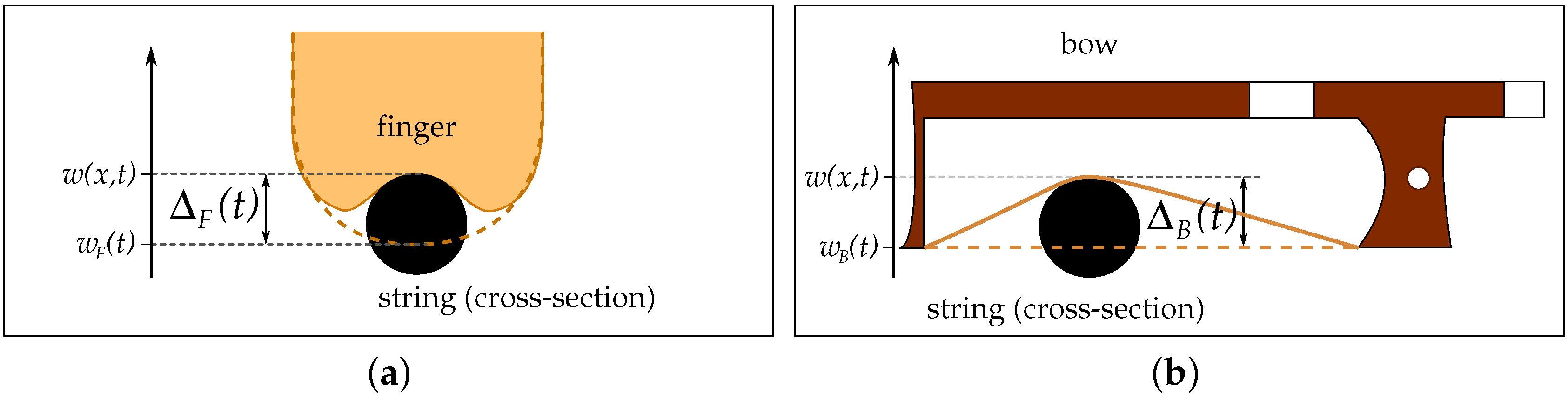
These contact forces are nonlinear functions of the penetration ${\Delta }_F\left(t\right)$ and ${\Delta }_B\left(t\right)$, corresponding to the distance by which the colliding object (here, the fingertip and the bow hair, respectively) would deform from its resting shape. Figure 2a,b provide a visual interpretation of the finger and the bow penetrations. ${\Delta }_F\left(t\right)$ and ${\Delta }_B\left(t\right)$ are defined as:

$${\Delta }_F\left(t\right)={\int }_{\mathcal{D}}{J}_F(x,t)w(x,t)dx-w_F\left(t\right)$$ (7a)

$${\Delta }_B\left(t\right)={\int }_{\mathcal{D}}{J}_B(x,t)w(x,t)dx-w_B\left(t\right)$$ (7b)

where $w_F\left(t\right)$ and $w_B\left(t\right)$ are respectively the vertical positions of the finger and bow at time t (see Figure 2).

${\mathrm{\Phi }}_F\left({\Delta }_F\right)$ and ${\mathrm{\Phi }}_B\left({\Delta }_B\right)$ are nonlinear potential functions, related to the stored collision energy. ${\mathrm{\Psi }}_F\left({\Delta }_F\right)$ and ${\mathrm{\Psi }}_B\left({\Delta }_B\right)$ are nonlinear damping coefficients. They can be written as:

$$\begin{array}{cc}\hfill {\mathrm{\Phi }}_F& =\frac{K_F}{{\mathsf{\alpha }}_F+1}{\left[{\Delta }_F\right]}_{+}^{{\mathsf{\alpha }}_F+1}\hfill \end{array}$$ (8a) $$\begin{array}{cc}\hfill {\mathrm{\Psi }}_F& =K_F{\mathsf{\beta }}_F{\left[{\Delta }_F\right]}_{+}^{{\mathsf{\alpha }}_F}\hfill \end{array}$$ (8b)

$$\begin{array}{cc}\hfill {\mathrm{\Phi }}_B& =\frac{K_B}{{\mathsf{\alpha }}_B+1}{\left[{\Delta }_B\right]}_{+}^{{\mathsf{\alpha }}_B+1}\hfill \end{array}$$ (9a) $$\begin{array}{cc}\hfill {\mathrm{\Psi }}_B& =K_B{\mathsf{\beta }}_B{\left[{\Delta }_B\right]}_{+}^{{\mathsf{\alpha }}_B}\hfill \end{array}$$ (9b)

where ${\left[·\right]}_{+}$ means $max(·,0)$.

The parameters $K_F$ and $K_B$, both strictly positive, define the respective stiffnesses of the finger and the bow. ${\mathsf{\alpha }}_F$ and ${\mathsf{\alpha }}_B$ are power law exponents, both larger than 1. ${\mathsf{\beta }}_F$ and ${\mathsf{\beta }}_B$ are positive damping factors.

$w_F\left(t\right)$ and $w_B\left(t\right)$ are respectively the vertical positions of the finger and bow at time t (see Figure 2). Their behaviour is governed by:

$$M_F{\ddot{w}}_F=f_F+f_{\mathrm{ext}w,F}$$ (10a)

$$M_B{\ddot{w}}_B=f_B+f_{\mathrm{ext}w,B}$$ (10b)

where $M_F$, $M_B$ are the finger and bow masses, respectively (in kg), and $f_{\mathrm{ext}w,F}\left(t\right)$, $f_{\mathrm{ext}w,B}\left(t\right)$ are the external forces applied vertically on the finger and bow, respectively (in N).

2.4.3. Fingerboard

The fingerboard forms a distributed barrier under the string. Equation (4) therefore generalises to:

$$\mathcal{L}w={\mathcal{F}}_N-J_F{f}_F-J_B{f}_B$$

(11)

where the index ${·}_N$ indicates “neck”, to avoid confusion.

${\mathcal{F}}_N$ is the contact force density exerted by the neck onto the string, along its length (in N/m). Here, the Hunt and Crossley collision model is used again, this time as a smooth approximation to a rigid collision:

$${\mathcal{F}}_N\left({\Delta }_N\right)=\frac{{\partial }_t{\mathrm{\Phi }}_N}{{\partial }_t{\Delta }_N}+{\partial }_t{\Delta }_N{\mathrm{\Psi }}_N$$

(12)

Once again, the contact force is a function of the fingerboard penetration ${\Delta }_N(x,t)$, defined over $\mathcal{D}$:

$${\Delta }_N(x,t)=\mathsf{\epsilon }\left(x\right)-w(x,t)$$

(13)

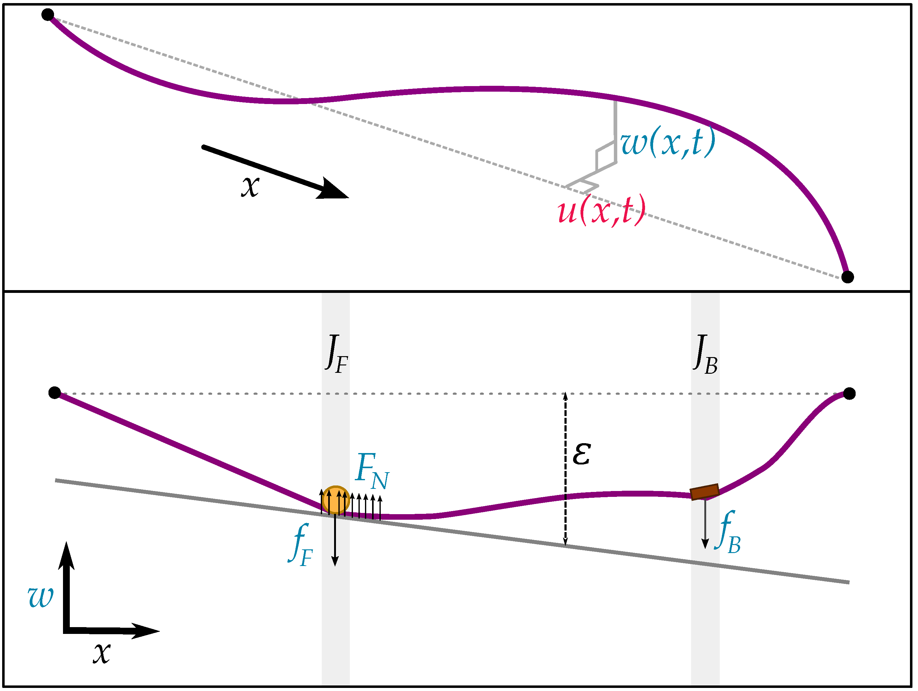
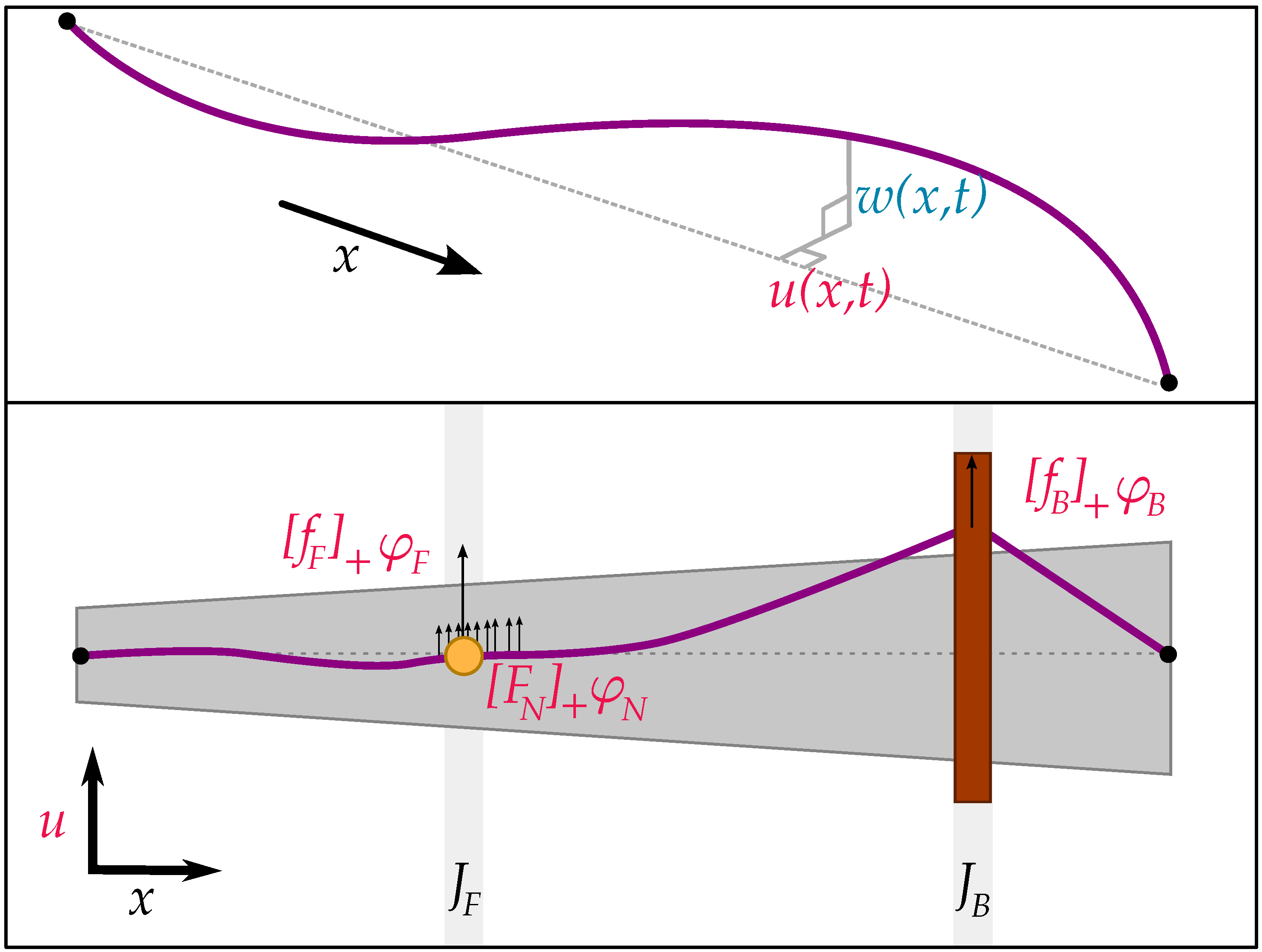
where $\mathsf{\epsilon }\left(x\right)$ is the position of the fingerboard with respect to the string at rest (i.e., the action of the instrument). Figure 3 summarises the forces at play in the vertical polarisation.

${\mathrm{\Phi }}_N\left({\Delta }_N\right)$ and ${\mathrm{\Psi }}_N\left({\Delta }_N\right)$ are defined analogously to the finger and bow functions in Equations (8) and (9):

$${\mathrm{\Phi }}_N=\frac{K_N}{{\mathsf{\alpha }}_N+1}{\left[{\Delta }_N\right]}_{+}^{{\mathsf{\alpha }}_N+1}$$ (14a)

$${\mathrm{\Psi }}_N=K_N{\mathsf{\beta }}_N{\left[{\Delta }_N\right]}_{+}^{{\mathsf{\alpha }}_N}$$ (14b)

where $K_N$ is chosen very large to approach an ideally rigid collision. Indeed, such a choice ensures that ${\Delta }_N$ stays very small, as should be for fingerboard-like structures [39].

2.5. Horizontal Polarisation

2.5.1. The Friction Interaction

The vertical contact forces described in Section 2.4 give rise to corresponding tangential friction forces onto the string, in the horizontal polarisation. A classic dry friction model is used, where the friction force is directly proportional to the normal force:

$$F_F={\left[F_C\right]}_{+}\mathsf{\phi }$$

(15)

where $F_F$ is the tangential friction force (in N), $\mathsf{\phi }$ is a dimensionless friction coefficient, and $F_C$ is the normal contact force, applied downwards on the string. The neck, finger and bow are not considered adhesive, therefore friction exists only for positive normal forces.

The friction force therefore arises from a friction coefficient, modulated by the normal force applied on the string. As a result, the interactions in the vertical polarisation feed into the horizontal polarisation. It is important to note that, for this particular framework, this is the coupling point between the two modelled directions; as mentioned earlier in Section 2.3, there is no other form of polarisation coupling in this model.

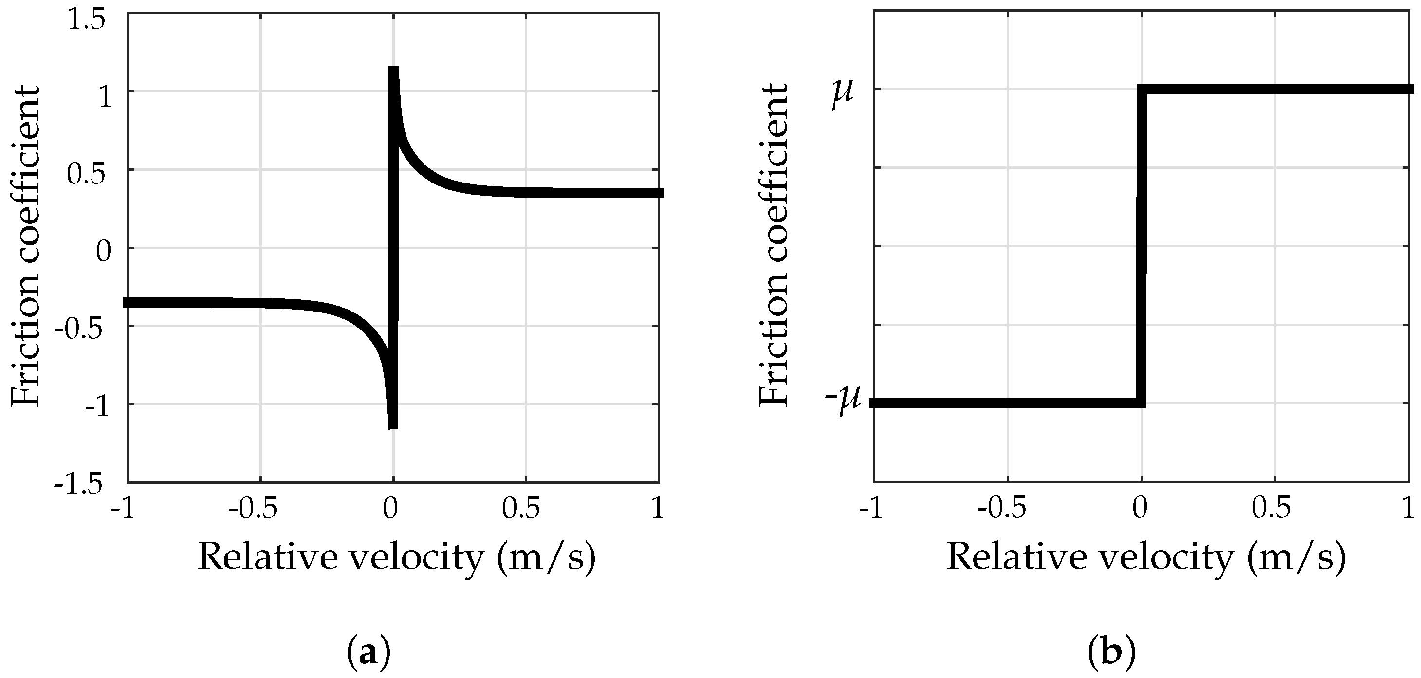
The friction coefficient can be defined as dependent on the relative velocity between the string and the external object. One can therefore establish a force-velocity friction curve, mapping the friction coefficient to a particular value of the relative velocity $v_{\mathrm{rel}}$.

2.5.2. Bow

The most straightforward way to introduce the tangential friction forces is probably to come back to the simple bowed string, where the friction phenomenon is the most appreciable. The bowed string equation in the horizontal polarisation is:

$$\mathcal{L}u=-J_B{\left[f_B\right]}_{+}{\mathsf{\phi }}_B$$

(16)

where $J_B(x,t)$ and $f_B\left(t\right)$ are the distribution and the normal collision force defined in Section 2.4.2. Note the negative sign in front of the friction term, reflecting the friction force opposing the motion of the string. ${\mathsf{\phi }}_B\left(v_{\mathrm{rel},B}\right)$ is a dimensionless friction coefficient, depending on $v_{\mathrm{rel},B}$, the relative velocity between the bow hair and the string. These are defined as [42]:

$$\begin{array}{cc}\hfill & \left\{\begin{array}{cc}|{\mathsf{\phi }}_B|⩽1.2\hfill & \mathrm{if} \left(v_{\mathrm{rel},B}\right)=0\hfill \\ {\mathsf{\phi }}_B=\mathrm{sign}\left(v_{\mathrm{rel},B}\right)\left(0.4e^{\frac{-|v_{\mathrm{rel},B}|}{0.01}}+0.45e^{\frac{-|v_{\mathrm{rel},B}|}{0.1}}+0.35\right)\hfill & \mathrm{if} v_{\mathrm{rel},B}\ne 0\left(\mathrm{kinetic}\right)\hfill \end{array}\right.\hfill \end{array}$$

(17a)

$$\begin{array}{cc}\hfill & v_{\mathrm{rel},B}\left(t\right)=\frac{d}{dt}\left({\int }_{\mathcal{D}}{J}_B(x,t)u(x,t)-u_B\left(t\right)\right)dx\hfill \end{array}$$

(17b)

where $u_B\left(t\right)$ is the bow transverse displacement. As the bow is pushed across the string, the equation governing the transverse motion of the bow is:

$$M_B{\ddot{u}}_B=-{\mathsf{\lambda }}_B{\dot{u}}_B+{\left[f_B\right]}_{+}{\mathsf{\phi }}_B+f_{\mathrm{ext}u,B}$$

(18)

${\mathsf{\lambda }}_B$ is a positive coefficient quantifying the linear energy absorption by the bow in the horizontal direction. The linear damping term is negligible compared to the friction term, when the string is in contact with the bow; indeed, this linear term mainly has a practical purpose in the numerical simulations, that is to avoid the bow drifting away when it is lifted from the string at the end of a note.

$f_{\mathrm{ext}u,B}\left(t\right)$ is the force with which the player pushes the bow tangentially, in order to establish the desired bow velocity. Note the slight difference with the usual control parameter in most bowed string studies; instead of directly imposing a bow velocity $v_B\left(t\right)$, the force applied by the player on the bow is used, resulting in a bow velocity ${\dot{u}}_B$.

The choice of a friction coefficient depending on relative velocity, ${\mathsf{\phi }}_B\left(v_{\mathrm{rel},B}\right)$, while already quite refined and fairly costly to model, is nonetheless somewhat of a trade-off between computational simplification and physical realism. More elaborate models for the bowed string friction interaction, involving viscothermal effects in the rosin layer coating the bow hair, can be used [13,14]; however, they require significantly more advanced implementations. Satisfying results and synthetic sound are obtained with the simple friction curve, although it has been shown that using a temperature-based friction model improves playability [25]. The friction curve employed here for the bow is deduced from experimental measurements in the steady sliding case (e.g., at constant velocity) [42]; it is illustrated in Figure 4a.

2.5.3. Finger

Adding the left hand finger in the horizontal direction yields:

$$\mathcal{L}u=-J_F{\left[f_F\right]}_{+}{\mathsf{\phi }}_F-J_B{\left[f_B\right]}_{+}{\mathsf{\phi }}_B$$

(19)

where $J_F(x,t)$ and $f_F\left(t\right)$ are defined in Section 2.4.2, and ${\mathsf{\phi }}_F\left(v_{\mathrm{rel},F}\right)$ is a dimensionless friction coefficient.

To the authors’ knowledge, there is no experimental data allowing for the calibration of the finger (or the fingerboard) friction curve. The fingers have the joint function, along with the fingerboard, of capturing the string to reduce its speaking length, to a crude approximation. In the absence of such data, a Coulomb-like step characteristic can therefore be assumed (illustrated in Figure 4b, where the static friction case occurs in most playing situations, but the string is capable of slipping under the finger if the left hand grip is too loose:

$$\begin{array}{cc}\hfill & \left\{\begin{array}{cc}|{\mathsf{\phi }}_F\left(v_{\mathrm{rel},F}\right)|⩽{\mathsf{\mu }}_F\hfill & \mathrm{if} v_{\mathrm{rel},F}=0\left(\mathrm{static}\right)\hfill \\ {\mathsf{\phi }}_F\left(v_{\mathrm{rel},F}\right)={\mathsf{\mu }}_F\mathrm{sign}\left(v_{\mathrm{rel},F}\right)\hfill & \mathrm{if} v_{\mathrm{rel},F}\ne 0\left(\mathrm{kinetic}\right)\hfill \end{array}\right.\hfill \end{array}$$

(20a)

$$\begin{array}{cc}\hfill & v_{\mathrm{rel},F}\left(t\right)=\frac{d}{dt}\left({\int }_{\mathcal{D}}{J}_F(x,t)u(x,t)-u_F\left(t\right)\right)dx\hfill \end{array}$$

(20b)

${\mathsf{\mu }}_F$ is a positive kinetic friction coefficient, quantifying how “sticky” the fingertip is. $u_F\left(t\right)$ is the horizontal position of the fingertip, with respect to the resting string axis. It is hypothesised that the fingertip oscillates about the top finger joint, while simultaneously damping the horizontal vibrations of the string. The temporal evolution of $u_F\left(t\right)$ can therefore be written as:

$$M_F{\ddot{u}}_F=-{\mathcal{K}}_F{u}_F-{\mathsf{\lambda }}_F{\dot{u}}_F+{\left[f_F\right]}_{+}{\mathsf{\phi }}_F$$

(21)

where ${\mathcal{K}}_F⩾0$ is a spring constant, and ${\mathsf{\lambda }}_F⩾0$ is a damping coefficient. A linear damped oscillator model for the finger is chosen in the horizontal polarisation. Indeed, the choice of a more elaborate contact model such as the one used in the vertical polarisation seems unjustified; while impacts are dominant in the vertical polarisation, e.g., when hammering the string for changing notes, it is clear that collisions only have an auxiliary effect in the tangential polarisation.

Note that this version of the model, before even introducing the fingerboard, could be used to simulate the bowing of natural harmonics of the string.

2.5.4. Fingerboard

The fingerboard friction force is distributed along the whole string; if plucked particularly hard, the string’s impact on the fingerboard can tangentially translate into friction, and the string will also slide against the neck of the instrument, adding to the audible rattling effect. The string equation becomes:

$$\mathcal{L}u=-{\left[{\mathcal{F}}_N\right]}_{+}{\mathsf{\phi }}_N-J_F{\left[f_F\right]}_{+}{\mathsf{\phi }}_F-J_B{\left[f_B\right]}_{+}{\mathsf{\phi }}_B$$

(22)

where, again, ${\mathcal{F}}_N(x,t)$ is the normal fingerboard force defined in Section 2.4.3, and ${\mathsf{\phi }}_N\left(v_{\mathrm{rel},N}\right)$ is the friction coefficient for the fingerboard, depending on the relative velocity between the fingerboard and the string (that is, the velocity of the string itself, as the fingerboard is not moving):

$$\begin{array}{cc}\hfill & \left\{\begin{array}{cc}|{\mathsf{\phi }}_N\left(v_{\mathrm{rel},N}\right)|⩽{\mathsf{\mu }}_N\hfill & \mathrm{if} v_{\mathrm{rel},N}=0\left(\mathrm{static}\right)\hfill \\ {\mathsf{\phi }}_N\left(v_{\mathrm{rel},N}\right)={\mathsf{\mu }}_N\mathrm{sign}\left(v_{\mathrm{rel},N}\right)\hfill & \mathrm{if} v_{\mathrm{rel},N}\ne 0\left(\mathrm{kinetic}\right)\hfill \end{array}\right.\hfill \end{array}$$

(23a)

$$\begin{array}{cc}\hfill & v_{\mathrm{rel},N}(x,t)={\partial }_{t}u\hfill \end{array}$$

(23b)

Figure 5 summarises the forces at play in the horizontal polarisation.

2.6. Energy Analysis

One can derive a power balance equation for both polarisations. The transfer of this equation to discrete time provides a tool to help ensure numerical stability.

Multiplying Equation (11) by ${\partial }_{t}w$ and integrating over the length of the string, and multiplying Equations (10a) and (10b) by ${\dot{w}}_F$ and ${\dot{w}}_B$ respectively, yield the following power balance (for energy-conserving boundary conditions, such as those given in Equation (3)):

$${\dot{H}}_w=P_w-Q_w$$

(24)

The variation of the total kinetic and potential energy $H_w\left(t\right)=H_{w,s}\left(t\right)+H_{w,N}\left(t\right)+H_{w,F}\left(t\right)+H_{w,B}\left(t\right)$ is equal to the total power $P_w\left(t\right)$ supplied to the system through external excitation (which can be negative), minus the power $Q_w\left(t\right)⩾0$ withdrawn from the system through damping. The system is therefore globally energy balanced. The energy is defined as:

$$\begin{array}{cc}\hfill H_w& =H_{w,s}+H_{w,N}+H_{w,F}+H_{w,B}\hfill \end{array}$$

(25a)

$$\begin{array}{cc}\hfill H_{w,s}& ={\int }_{{\mathcal{D}}_{\mathcal{S}}}\left[\frac{\mathsf{\rho }}{2}{\left({\partial }_{t}w\right)}^2+\frac{T}{2}{\left({\partial }_{x}w\right)}^2+\frac{E{I}_0}{2}{\left({\partial }_x^{2}w\right)}^2\right]dx\hfill \end{array}$$

(25b)

$$\begin{array}{cc}\hfill H_{w,N}& ={\int }_{{\mathcal{D}}_{\mathcal{S}}}{\mathrm{\Phi }}_{N}dx\hfill \end{array}$$

(25c)

$$\begin{array}{cc}\hfill H_{w,F,B}& ={\mathrm{\Phi }}_{F,B}+\frac{M_{F,B}}{2}{\dot{w}}_{F,B}^2\hfill \end{array}$$

(25d)

The power supplied through external excitation is:

$$P_w={\dot{w}}_F{f}_{\mathrm{ext}w,F}+{\dot{w}}_B{f}_{\mathrm{ext}w,B}+{\int }_{{\mathcal{D}}_{\mathcal{S}}}\left(f_{F}w{\partial }_t{J}_F+f_{B}w{\partial }_t{J}_B\right)dx$$

(26)

The power lost through damping within the string and through collision with the neck, finger and bow is given by:

$$\begin{array}{cc}\hfill Q_w& =Q_{w,s}+Q_{\mathrm{\Psi }}\hfill \end{array}$$

(27a)

$$\begin{array}{cc}\hfill Q_{w,s}& =\mathsf{\rho }{\int }_{{\mathcal{D}}_{\mathcal{S}}}\left[{\mathsf{\lambda }}_1{\left({\partial }_{t}w\right)}^2+{\mathsf{\lambda }}_2{\left({\partial }_t{\partial }_{x}w\right)}^2\right]dx\hfill \end{array}$$

(27b)

$$\begin{array}{cc}\hfill Q_{\mathrm{\Psi }}& ={\int }_{{\mathcal{D}}_{\mathcal{S}}}{\left({\partial }_t{\Delta }_N\right)}^2{\mathrm{\Psi }}_{N}dx+{\dot{\Delta }}_F^2{\mathrm{\Psi }}_F+{\dot{\Delta }}_B^2{\mathrm{\Psi }}_B\hfill \end{array}$$

(27c)

In the absence of excitation, the energy $H_w$ strictly decreases.

For the horizontal polarisation, multiplying Equation (22) by ${\partial }_{t}u$ and integrating over ${\mathcal{D}}_{\mathcal{S}}$, and multiplying Equations (18) and (21) by ${\dot{u}}_B$ and ${\dot{u}}_F$ respectively, yield the power balance:

$${\dot{H}}_u=P_u-Q_u$$

(28)

Again, the variation of $H_u\left(t\right)=H_{u,s}\left(t\right)+H_{u,F}\left(t\right)+H_{u,B}\left(t\right)$ is equal to the total power $P_u\left(t\right)$ supplied to the system in the horizontal polarisation through external excitation, minus power losses $Q_u\left(t\right)⩾0$ from damping. The energy is defined as:

$$\begin{array}{cc}\hfill H_u& =H_{u,s}+H_{u,F}+H_{u,B}\hfill \end{array}$$

(29a)

$$\begin{array}{cc}\hfill H_{u,s}& ={\int }_{{\mathcal{D}}_{\mathcal{S}}}\left[\frac{\mathsf{\rho }}{2}{\left({\partial }_{t}u\right)}^2+\frac{T}{2}{\left({\partial }_{x}u\right)}^2+\frac{E{I}_0}{2}{\left({\partial }_x^{2}u\right)}^2\right]dx\hfill \end{array}$$

(29b)

$$\begin{array}{cc}\hfill H_{u,F}& =\frac{M_F}{2}{\dot{u}}_F^2+\frac{{\mathcal{K}}_F}{2}{u}_F^2\hfill \end{array}$$

(29c)

$$\begin{array}{cc}\hfill H_{u,B}& =\frac{M_B}{2}{\dot{u}}_B^2\hfill \end{array}$$

(29d)

The power supplied or withdrawn by external excitation is:

$$P_u={\left[f_F\right]}_{+}{\mathsf{\phi }}_F{\int }_{{\mathcal{D}}_{\mathcal{S}}}u{\partial }_t{J}_{F}dx+{\left[f_B\right]}_{+}{\mathsf{\phi }}_B{\int }_{{\mathcal{D}}_{\mathcal{S}}}u{\partial }_t{J}_{B}dx+{\dot{u}}_B{f}_{\mathrm{ext}u,B}$$

(30)

The power lost through string damping and friction is:

$$\begin{array}{cc}\hfill Q_u& =Q_{u,s}+Q_{\mathsf{\phi }}+Q_{u,F}+Q_{u,B}\hfill \end{array}$$

(31a)

$$\begin{array}{cc}\hfill Q_{u,s}& =\mathsf{\rho }{\int }_{{\mathcal{D}}_{\mathcal{S}}}\left[{\mathsf{\lambda }}_1{\left({\partial }_{t}u\right)}^2+{\mathsf{\lambda }}_2{\left({\partial }_t{\partial }_{x}u\right)}^2\right]dx\hfill \end{array}$$

(31b)

$$\begin{array}{cc}\hfill Q_{\mathsf{\phi }}& ={\int }_{{\mathcal{D}}_{\mathcal{S}}}{v}_{\mathrm{rel},N}{\left[{\mathcal{F}}_N\right]}_{+}{\mathsf{\phi }}_{N}dx+v_{\mathrm{rel},F}{\left[f_F\right]}_{+}{\mathsf{\phi }}_F+v_{\mathrm{rel},B}{\left[f_B\right]}_{+}{\mathsf{\phi }}_B\hfill \end{array}$$

(31c)

$$\begin{array}{cc}\hfill Q_{u,F,B}& ={\mathsf{\lambda }}_{F,B}{\dot{u}}_{F,B}^2\hfill \end{array}$$

(31d)

Note that $Q_u⩾0$ if $v_{\mathrm{rel}}\mathsf{\phi }\left(v_{\mathrm{rel}}\right)⩾0$, which is true for the friction characteristics of the three objects.

The total power of the full system is therefore balanced by:

$$\dot{H}=P-Q$$ (32a)

$$H=H_u+H_w$$ (32b)

$$P=P_u+P_w$$ (32c)

$$Q=Q_u+Q_w$$ (32d)

A power balance of the same type as Equation (32a) is generally used as the base for another class of modelling methods, based on so-called port-Hamiltonian systems [54]. Discretisation of such systems has recently been successfully implemented for time domain physical modelling of acoustic and electroacoustic systems [55].

3. Numerical Scheme

3.1. Framework

3.1.1. Discretising the Equations of Motion

The equations of motion can now be discretised by approximating the partial derivatives with their finite difference [17] counterparts. This method allows a full system simulation, and therefore great flexibility of control for the input parameters and gesture reproduction, at the cost of increased computational requirements. This method has seen a myriad of applications in physical modelling sound synthesis, and more generally musical acoustics simulations [3,18]. In this section, the numerical scheme is defined, the discrete energy balance is detailed, and the scheme update is described.

3.1.2. Grid Functions and Finite Difference (FD) Operators

All the time varying quantities defined in Section 2 are now discretised into series of integer multiples of the time step, and defined at times $t=nk,n\in \mathbb{N}$. k is the time step in s; $F_s=k^{-1}$ is the desired sample rate in Hz. Typically, audio sample rates are used, such as $F_s=44.1$ kHz.

The space dependent variables are discretised into grid functions, defined at positions $x=lh,l\in \mathfrak{D}=\left[0,\cdots ,N_{\mathfrak{D}}\right]$, where h is the grid spacing, in m.

For an arbitrary continuous function $g(x,t)$ defined for $x\in \mathcal{D}$ and $t\in {\mathbb{R}}^{+}$, $g_l^n$ is a grid function approximating $g(lh,nk)$, at grid point l and time step n. Introduce the forward and backward unit time and space shift operators, applied to $g_l^n$:

$$\begin{array}{cc}\hfill e_{t-}{g}_l^n& =g_l^{n-1}\hfill \end{array}$$ $$\begin{array}{cc}\hfill e_{t+}{g}_l^n& =g_l^{n+1}\hfill \end{array}$$	(33a)	$$\begin{array}{cc}\hfill e_{x-}{g}_l^n& =g_{l-1}^n\hfill \end{array}$$ $$\begin{array}{cc}\hfill e_{x+}{g}_l^n& =g_{l+1}^n\hfill \end{array}$$	(34a)
	(33b)		(34b)

Partial differentiation with respect to time and space can be approximated with a number of first order Finite Difference (FD) operators:

$$\begin{array}{cc}\hfill {\mathsf{\delta }}_{t-}& =\frac{1-e_{t-}}{k}\hfill \end{array}$$ $$\begin{array}{cc}\hfill {\mathsf{\delta }}_{t+}& =\frac{e_{t+}-1}{k}\hfill \end{array}$$ $$\begin{array}{cc}\hfill {\mathsf{\delta }}_{t·}& =\frac{e_{t+}-e_{t-}}{2k}\hfill \end{array}$$	(35a)	$${\mathsf{\delta }}_{x-}=\frac{1-e_{x-}}{h}$$	(36a)
	(35b)	$${\mathsf{\delta }}_{x+}=\frac{e_{x+}-1}{h}$$	(36b)
	(35c)

Higher order partial derivation operators are approximated with:

$${\partial }_t^2\approx {\mathsf{\delta }}_{tt}={\mathsf{\delta }}_{t-}{\mathsf{\delta }}_{t+}$$ (37a)

$${\partial }_x^2\approx {\mathsf{\delta }}_{xx}={\mathsf{\delta }}_{x-}{\mathsf{\delta }}_{x+}$$ (37b)

Finally, the averaging FD operators approximate identity:

$${\mathsf{\mu }}_{t-}=\frac{1+e_{t-}}{2}$$ (38a)

$${\mathsf{\mu }}_{t+}=\frac{e_{t+}+1}{2}$$ (38b)

$${\mathsf{\mu }}_{t·}=\frac{e_{t+}+e_{t-}}{2}$$ (38c)

Note that ${\mathsf{\delta }}_{t-}{\mathsf{\mu }}_{t+}={\mathsf{\delta }}_{t+}{\mathsf{\mu }}_{t-}={\mathsf{\delta }}_{t·}$.

3.2. The Isolated String

3.2.1. Finite Difference Scheme

The discrete counterparts of $w(x,t)$ and $u(x,t)$ are the grid functions $w_l^n$ and $u_l^n$, as described in Section 3.1.2. System Equation (1) is discretised as:

$$\mathsf{L}{w}_l^n=0$$ (39a)

$$\mathsf{L}{u}_l^n=0$$ (39b)

where $\mathsf{L}$ is a finite difference discretisation of the differential operator $\mathcal{L}$ defined in Equation (2), using the finite difference operators described in Section 3.1.2:

$$\mathsf{L}=\mathsf{\rho }{\mathsf{\delta }}_{tt}-T{\mathsf{\delta }}_{xx}+E{I}_0{\mathsf{\delta }}_{xx}{\mathsf{\delta }}_{xx}+{\mathsf{\lambda }}_1\mathsf{\rho }{\mathsf{\delta }}_{t·}-{\mathsf{\lambda }}_2\mathsf{\rho }{\mathsf{\delta }}_{t-}{\mathsf{\delta }}_{xx}$$

(40)

The use of the backward first order time FD operator in the second damping term allows for the isolated string scheme to stay explicit; this results in simplified computations, at the cost of a slightly altered stability condition.

The discrete simply supported boundary conditions are given as:

$$\begin{array}{cc}\hfill w_0^n& =w_{N_{\mathfrak{D}}}^n=0\hfill \end{array}$$ $$\begin{array}{cc}\hfill {\mathsf{\delta }}_{xx}{w}_0^n& ={\mathsf{\delta }}_{xx}{w}_{N_{\mathfrak{D}}}^n=0\hfill \end{array}$$	(41a)	$$\begin{array}{cc}\hfill u_0^n& =u_{N_{\mathfrak{D}}}^n=0\hfill \end{array}$$ $$\begin{array}{cc}\hfill {\mathsf{\delta }}_{xx}{u}_0^n& ={\mathsf{\delta }}_{xx}{u}_{N_{\mathfrak{D}}}^n=0\hfill \end{array}$$	(42a)
	(41b)		(42b)

3.2.2. Vector-Matrix Notation

The grid functions $w_l^n$ and $u_l^n$ are defined over the discrete domain $\mathfrak{D}$, containing $N_{\mathfrak{D}}+1$ grid points. The discrete position of the whole string can therefore be described with vectors of length $N_{\mathfrak{D}}+1$. The first set of boundary conditions, Equations (41a) and (42a), ensure that the two extreme values of such vectors (i.e., the string displacement at the bridge and nut boundary) are 0 at all times. One now only needs to store the state of the string in a vector of size $(N_{\mathfrak{D}}-1)$, omitting these two extreme values:

$${\mathbf{w}}^n={\left[w_1^n,\cdots ,w_{N-1}^n\right]}^{\mathsf{T}}$$ (43a)

$${\mathbf{u}}^n={\left[u_1^n,\cdots ,u_{N-1}^n\right]}^{\mathsf{T}}$$ (43b)

The action of spatial FD operators on the grid functions is then equivalent to a matrix-vector multiplication. For simply supported boundary conditions, the notation of spatial FD operators in matrix form naturally follows as:

$${\mathbf{D}}_{x-}=\frac{1}{h}\left[\begin{array}{cccc}1& & & \\ -1& 1& & \\ & \ddots & \ddots & \\ & & -1& 1\\ & & & -1\end{array}\right]$$	(44a)	$$\begin{array}{c}\hfill \end{array}$$ $$\begin{array}{cc}\hfill & {\mathbf{D}}_{x+}=-{\mathbf{D}}_{x-}^{\mathsf{T}}\hfill \\ \hfill \end{array}$$ $$\begin{array}{cc}\hfill & {\mathbf{D}}_{xx}={\mathbf{D}}_{x+}{\mathbf{D}}_{x-}\hfill \end{array}$$	(44b)
			(44c)

of size $N_{\mathfrak{D}}\times (N_{\mathfrak{D}}-1)$, $(N_{\mathfrak{D}}-1)\times N_{\mathfrak{D}}$, $(N_{\mathfrak{D}}-1)\times (N_{\mathfrak{D}}-1)$, and $(N_{\mathfrak{D}}-1)\times (N_{\mathfrak{D}}-1)$, respectively.

System Equation (39) can now be written as a pair of vector equations:

$$\mathbf{L}{\mathbf{w}}^n=0$$ (45a)

$$\mathbf{L}{\mathbf{u}}^n=0$$ (45b)

where $\mathbf{L}$ is the matrix form of the difference operator $\mathsf{L}$ defined in Equation (40):

$$\mathbf{L}=\mathsf{\rho }{\mathsf{\delta }}_{tt}-T{\mathbf{D}}_{xx}+E{I}_0{\mathbf{D}}_{xx}{\mathbf{D}}_{xx}+{\mathsf{\lambda }}_1\mathsf{\rho }{\mathsf{\delta }}_{t·}-{\mathsf{\lambda }}_2\mathsf{\rho }{\mathsf{\delta }}_{t-}{\mathbf{D}}_{xx}$$

(46)

3.3. Vertical Polarisation

3.3.1. Discrete System

A discretisation for Equation (11) can now be written in vector-matrix form:

$$\mathbf{L}{\mathbf{w}}^n={\mathsf{\mu }}_{t·}{\mathbf{J}}_{\mathbf{w}}^n{\mathbf{f}}_{\mathbf{w}}^n$$

(47)

where ${\mathbf{J}}_{\mathbf{w}}^n$ is the $(N_{\mathfrak{D}}-1)\times (N_{\mathfrak{D}}+1)$ distribution matrix, and ${\mathbf{f}}_{\mathbf{w}}^n$ is a column vector containing all the contact force information:

$${\mathbf{J}}_{\mathbf{w}}^n=\left[\begin{array}{ccc}{\mathbf{I}}_{\mathbf{N}-\mathbf{1}}& -{\mathbf{j}}_F^n& -{\mathbf{j}}_B^n\end{array}\right]$$ (48a)

$${\mathbf{f}}_{\mathbf{w}}^n={\left[\begin{array}{ccc}{\left({\mathbf{f}}_N^n\right)}^{\mathsf{T}}& f_F^n& f_B^n\end{array}\right]}^{\mathsf{T}}$$ (48b)

where ${\mathbf{I}}_{\mathbf{N}-\mathbf{1}}$ is the $(N_{\mathfrak{D}}-1)\times (N_{\mathfrak{D}}-1)$ identity matrix, and ${\mathbf{j}}_F^n$ and ${\mathbf{j}}_B^n$ are discrete spreading operators in column vector form, accounting for the continuous distributions described in Section 2.4.2. If the contact regions are sufficiently wide, these can be sampled from the true shape of the concerned object; otherwise, if contact is localised in a small region, or pointwise, interpolation is needed between grid points, as truncation to the nearest grid point would result in audible artefacts when the finger or bow move along the length of the string.

The spreading vectors are normalised over the grid: for instance, in the simplified case of a fixed position object, located on a grid point, if $J_F(x,t)$ and $J_B(x,t)$ are Dirac delta functions, then ${\mathbf{j}}_F^n$ and ${\mathbf{j}}_B^n$ will be all-zero vectors, except for one element of value $\frac{1}{h}$, at the position where the force is applied.

Note the use of the averaging operator ${\mathsf{\mu }}_{t·}$ in Equation (47), necessary to show an energy balance for this scheme in the case of moving finger or bow (see Section 3.5).

${\mathbf{f}}_N^n$, $f_F^n$ and $f_B^n$ are the discrete counterparts of those defined in Section 2.4.2 and Section 2.4.3.

3.3.2. Collision Normal Forces

The force vector ${\mathbf{f}}_{\mathbf{w}}^n$ can be written as:

$${\mathbf{f}}_{\mathbf{w}}^n=\frac{{\mathsf{\delta }}_{t·}{\mathbf{\Phi }}^n}{{\mathsf{\delta }}_{t·}{\mathbf{\Delta }}^n}+\left({\mathsf{\delta }}_{t·}{\mathbf{\Delta }}^n\right)\odot {\mathbf{\Psi }}^n$$

(49)

where the division is pointwise, and ⊙ is the pointwise product. This expression for ${\mathbf{f}}_{\mathbf{w}}^n$ is written as a function of the vector penetration ${\mathbf{\Delta }}^n$, defined as:

$${\mathbf{\Delta }}^n=\left[\begin{array}{c}⋮\\ {\mathbf{\Delta }}_N^n\\ ⋮\\ {\Delta }_F^n\\ {\Delta }_B^n\end{array}\right]$$	(50a)	$$\begin{array}{cc}\hfill {\mathbf{\Delta }}_N^n& =\mathbf{\epsilon }-{\mathbf{w}}^n\hfill \end{array}$$ $$\begin{array}{cc}\hfill {\Delta }_F^n& =h{{\mathbf{j}}_F^n}^{\mathsf{T}}{\mathbf{w}}^n-w_F^n\hfill \end{array}$$ $$\begin{array}{cc}\hfill {\Delta }_B^n& =h{{\mathbf{j}}_B^n}^{\mathsf{T}}{\mathbf{w}}^n-w_B^n\hfill \end{array}$$	(50b)
			(50c)
			(50d)

where the elements of vector $\mathbf{\epsilon }$ are ${\mathsf{\epsilon }}_l=\mathsf{\epsilon }\left(lh\right)$, and $w_F^n$ and $w_B^n$ are the respective vertical positions of the finger and bow.

${\mathbf{\Phi }}^n\left({\mathbf{\Delta }}^n\right)$, ${\mathbf{\Psi }}^n\left({\mathbf{\Delta }}^n\right)$ are now vector functions of ${\mathbf{\Delta }}^n$:

$${\mathbf{\Phi }}^n\left({\mathbf{\Delta }}^n\right)=\frac{K}{\mathbf{\alpha }+1}\odot {\left[{\mathbf{\Delta }}^n\right]}_{+}^{\mathbf{\alpha }+1}$$ (51a)

$${\mathbf{\Psi }}^n\left({\mathbf{\Delta }}^n\right)=K\odot \mathbf{\beta }\odot {\left[{\mathbf{\Delta }}^n\right]}_{+}^{\mathbf{\alpha }}$$ (51b)

where the exponentiation operation is also element-wise, and the nonlinearity parameters K, $\mathsf{\alpha }$, and $\mathsf{\beta }$ are themselves in vector form:

$$K=\left[\begin{array}{c}⋮\\ K_N\\ ⋮\\ K_F\\ K_B\end{array}\right]$$ (52a)

$$\mathbf{\alpha }=\left[\begin{array}{c}⋮\\ {\mathsf{\alpha }}_N\\ ⋮\\ {\mathsf{\alpha }}_F\\ {\mathsf{\alpha }}_B\end{array}\right]$$ (52b)

$$\mathbf{\beta }=\left[\begin{array}{c}⋮\\ {\mathsf{\beta }}_N\\ ⋮\\ {\mathsf{\beta }}_F\\ {\mathsf{\beta }}_B\end{array}\right]$$ (52c)

Finally, the discrete equations for the evolution of the vertical positions of the finger and bow can be written as:

$${\mathbf{M}}_{FB}{\mathsf{\delta }}_{tt}{\mathbf{w}}_{FB}^n={\mathbf{f}}_{\mathbf{w}FB}^n+{\mathbf{f}}_{\mathbf{ext}w,FB}^n$$

(53a)

$${\mathbf{M}}_{FB}=\left[\begin{array}{c}{M}_{F}0\\ 0M_B\end{array}\right]$$ (53b)

$${\mathbf{w}}_{FB}^n=\left[\begin{array}{c}{w}_F^n\\ w_B^n\end{array}\right]$$ (53c)

$${\mathbf{f}}_{\mathbf{w}FB}^n=\left[\begin{array}{c}{f}_F^n\\ f_B^n\end{array}\right]$$ (53d)

$${\mathbf{f}}_{\mathbf{ext}w,FB}^n=\left[\begin{array}{c}{f}_{\mathrm{ext}w,F}^n\\ f_{\mathrm{ext}w,B}^n\end{array}\right]$$ (53e)

3.4. Horizontal Polarisation

Equation (22) is now discretised as:

$$\mathbf{L}{\mathbf{u}}^n=-{\mathsf{\mu }}_{t·}{\mathbf{J}}_{\mathbf{u}}^n{\mathbf{f}}_{\mathbf{u}}^n$$ (54a)

$${\mathbf{J}}_{\mathbf{u}}^n=\left[\begin{array}{ccc}{\mathbf{I}}_{\mathbf{N}-\mathbf{1}}& {\mathbf{j}}_F^n& {\mathbf{j}}_B^n\end{array}\right]$$ (54b)

$\mathbf{L}$ is defined in Equation (46). ${\mathbf{f}}_{\mathbf{u}}^n$ is a column vector containing the friction force information:

$${\mathbf{f}}_{\mathbf{u}}^n={\left[{\mathbf{f}}_{\mathbf{w}}^n\right]}_{+}\odot \left[\begin{array}{c}⋮\\ {\mathsf{\phi }}_N\left({\mathbf{v}}_{\mathrm{rel},N}^n\right)\\ ⋮\\ {\mathsf{\phi }}_F\left(v_{\mathrm{rel},F}^n\right)\\ {\mathsf{\phi }}_B\left(v_{\mathrm{rel},B}^n\right)\end{array}\right]$$	(55a)	$$\begin{array}{cc}\hfill {\mathbf{v}}_{\mathrm{rel},N}^n& ={\mathsf{\delta }}_{t·}{\mathbf{u}}^n\hfill \end{array}$$ $$\begin{array}{cc}\hfill v_{\mathrm{rel},F}^n& =h{\mathsf{\delta }}_{t·}\left({{\mathbf{j}}_F^n}^{\mathsf{T}}{\mathbf{u}}^n\right)-{\mathsf{\delta }}_{t·}{u}_F^n\hfill \end{array}$$ $$\begin{array}{cc}\hfill v_{\mathrm{rel},B}^n& =h{\mathsf{\delta }}_{t·}\left({{\mathbf{j}}_B^n}^{\mathsf{T}}{\mathbf{u}}^n\right)-{\mathsf{\delta }}_{t·}{u}_B^n\hfill \end{array}$$	(55b)
			(55c)
			(55d)

where ${\mathsf{\phi }}_N$, ${\mathsf{\phi }}_F$ and ${\mathsf{\phi }}_B$ are defined in Section 2.5. One can define a vector relative velocity:

$${\mathbf{v}}_{\mathrm{rel}}^n={\left[\begin{array}{c}{\left({\mathbf{v}}_{\mathrm{rel},N}^n\right)}^{\mathsf{T}}\left|v_{\mathrm{rel},F}^n\right|v_{\mathrm{rel},B}^n\end{array}\right]}^{\mathsf{T}}$$

(56)

Finally, a matrix equation describes the evolution of the horizontal displacements $u_F^n$ and $u_B^n$ of the finger and bow, respectively:

$${\mathbf{M}}_{FB}{\mathsf{\delta }}_{tt}{\mathbf{u}}_{FB}^n={\mathbf{K}}_{FB}{\mathsf{\mu }}_{t·}{\mathbf{u}}_{FB}^n-{\mathbf{\lambda }}_{FB}{\mathsf{\delta }}_{t·}{\mathbf{u}}_{FB}^n+{\mathbf{f}}_{\mathbf{u}FB}^n+{\mathbf{f}}_{\mathbf{ext}u,FB}^n$$

(57a)

$${\mathbf{K}}_{FB}=\left[\begin{array}{c}{\mathcal{K}}_{F}0\\ 00\end{array}\right]$$ (57b)

$${\mathbf{\lambda }}_{FB}=\left[\begin{array}{c}{\mathsf{\lambda }}_{F}0\\ 0{\mathsf{\lambda }}_B\end{array}\right]$$ (57c)

$${\mathbf{u}}_{FB}^n=\left[\begin{array}{c}{u}_F^n\\ u_B^n\end{array}\right]$$ (57d)

$${\mathbf{f}}_{\mathbf{u}FB}^n={\left[{\mathbf{f}}_{\mathbf{w}FB}^n\right]}_{+}\odot \left[\begin{array}{c}{\mathsf{\phi }}_F\left(v_{\mathrm{rel},F}^n\right)\\ {\mathsf{\phi }}_B\left(v_{\mathrm{rel},B}^n\right)\end{array}\right]$$ (57e)

$${\mathbf{f}}_{\mathbf{ext}u,FB}^n=\left[\begin{array}{c}0\\ f_{\mathrm{ext}u,B}^n\end{array}\right]$$ (57f)

where the 2-point averaging operator ${\mathsf{\mu }}_{t·}$ is used as a means to avoid restricting the stability limit of this scheme any further; this aspect will be developed in Section 3.5.4.

3.5. Energy Analysis

The results of Section 2.6 can be transferred to discrete time, and the energy exchanges going on in the system can be monitored at all times during the simulation. An energy balance equation is derived between the energy of the closed system (${\mathrm{H}}^n$) and the power brought in and out, by external excitation (${\mathrm{P}}^n$) and damping ${\mathrm{Q}}^n$. The maintenance of this energy balance is a means to ensure a stable algorithm.

3.5.1. Vertical Polarisation

For the vertical polarisation, multiplying Equation (47) by $h{\left({\mathsf{\delta }}_{t·}{\mathbf{w}}^n\right)}^{\mathsf{T}}$ and Equation (53a) by ${\left({\mathsf{\delta }}_{t·}{\mathbf{w}}_{FB}^n\right)}^{\mathsf{T}}$ gives the power balance:

$${\mathsf{\delta }}_{t-}{\mathrm{H}}_w^n={\mathrm{P}}_w^n-{\mathrm{Q}}_w^n$$

(58)

The numerical energy ${\mathrm{H}}_w^n$ is defined as:

$$\begin{array}{cc}\hfill & {\mathrm{H}}_w^n={\mathrm{H}}_{w,s}^n+{\mathrm{H}}_{\mathrm{\Phi }}^n\hfill \end{array}$$

(59a)

$$\begin{array}{cc}\hfill {\mathrm{H}}_{w,s}^n& =\frac{\mathsf{\rho }h}{2}{\left|{\mathsf{\delta }}_{t+}{\mathbf{w}}^n\right|}^2+\frac{Th}{2}{\left({\mathbf{D}}_{x-}{\mathbf{w}}^n\right)}^{\mathsf{T}}{\mathbf{D}}_{x-}{\mathbf{w}}^{n+1}+\frac{E{I}_{0}h}{2}{\left({\mathbf{D}}_{xx}{\mathbf{w}}^n\right)}^{\mathsf{T}}{\mathbf{D}}_{xx}{\mathbf{w}}^{n+1}\hfill \\ & -\frac{{\mathsf{\lambda }}_2\mathsf{\rho }kh}{4}{\left|{\mathsf{\delta }}_{t+}{\mathbf{D}}_{x-}{\mathbf{w}}^n\right|}^2\hfill \end{array}$$

(59b)

$$\begin{array}{cc}\hfill & {\mathrm{H}}_{\mathrm{\Phi }}^n={\mathbf{h}}^{\mathsf{T}}{\mathsf{\mu }}_{t+}{\mathbf{\Phi }}^n+\frac{1}{2}{\left({\mathbf{M}}_{FB}{\mathsf{\delta }}_{t+}{\mathbf{w}}_{FB}^n\right)}^{\mathsf{T}}{\mathsf{\delta }}_{t+}{\mathbf{w}}_{FB}^n\hfill \end{array}$$

(59c)

where $\mathbf{h}={[\cdots h\cdots |1\left|1\right]}^{\mathsf{T}}$.

The power ${\mathrm{P}}_w^n$ supplied or withdrawn through excitation is:

$${\mathrm{P}}_w^n={\left({\mathsf{\delta }}_{t·}{\mathbf{w}}_{FB}^n\right)}^{\mathsf{T}}{\mathbf{f}}_{\mathrm{ext}w,FB}^n-h\left({\left({\mathsf{\mu }}_{t·}{\mathbf{w}}^n\right)}^{\mathsf{T}}\left({\mathsf{\delta }}_{t·}{\mathbf{J}}^n\right)\right){\mathbf{f}}_{\mathbf{w}}^n$$

(60)

The power ${\mathrm{Q}}_w^n⩾0$ dissipated through damping is:

$$\begin{array}{cc}\hfill & {\mathrm{Q}}_w^n={\mathrm{Q}}_{w,s}^n+{\mathrm{Q}}_{\mathrm{\Psi }}^n\hfill \end{array}$$

(61a)

$$\begin{array}{cc}\hfill & {\mathrm{Q}}_{w,s}^n={\mathsf{\lambda }}_1\mathsf{\rho }h|{\mathsf{\delta }}_{t·}{\mathbf{w}}^n{|}^2+{\mathsf{\lambda }}_2\mathsf{\rho }h{\left|{\mathsf{\delta }}_{t·}{\mathbf{D}}_{x-}{\mathbf{w}}^n\right|}^2\hfill \end{array}$$

(61b)

$$\begin{array}{cc}\hfill & {\mathrm{Q}}_{\mathrm{\Psi }}^n={\left(\mathbf{h}\odot {\mathsf{\delta }}_{t·}{\mathbf{\Delta }}^n\right)}^{\mathsf{T}}\left(\left({\mathsf{\delta }}_{t·}{\mathbf{\Delta }}^n\right)\odot {\mathbf{\Psi }}^n\right)\hfill \end{array}$$

(61c)

In the absence of external excitation, the numerical energy ${\mathrm{H}}_w^n$ is strictly decreasing.

3.5.2. Horizontal Polarisation

On the other hand, the product of Equation (54a) by $h{\left({\mathsf{\delta }}_{t·}{\mathbf{u}}^n\right)}^{\mathsf{T}}$, and that of Equation (57a) by ${\left({\mathsf{\delta }}_{t·}{\mathbf{u}}_{FB}^n\right)}^{\mathsf{T}}$, yield a numerical power balance for the horizontal polarisation:

$${\mathsf{\delta }}_{t-}{\mathrm{H}}_u^n={\mathrm{P}}_u^n-{\mathrm{Q}}_u^n$$

(62)

where the numerical energy ${\mathrm{H}}_u^n$ is defined as:

$$\begin{array}{cc}\hfill & {\mathrm{H}}_u^n={\mathrm{H}}_{u,s}^n+{\mathrm{H}}_{u,FB}^n\hfill \end{array}$$

(63a)

$$\begin{array}{cc}\hfill {\mathrm{H}}_{u,s}^n& =\frac{\mathsf{\rho }h}{2}{\left|{\mathsf{\delta }}_{t+}{\mathbf{u}}^n\right|}^2+\frac{Th}{2}{\left({\mathbf{D}}_{x-}{\mathbf{u}}^n\right)}^{\mathsf{T}}{\mathbf{D}}_{x-}{\mathbf{u}}^{n+1}+\frac{E{I}_{0}h}{2}{\left({\mathbf{D}}_{xx}{\mathbf{u}}^n\right)}^{\mathsf{T}}{\mathbf{D}}_{xx}{\mathbf{u}}^{n+1}\hfill \\ & -\frac{{\mathsf{\lambda }}_2\mathsf{\rho }kh}{4}{\left|{\mathsf{\delta }}_{t+}{\mathbf{D}}_{x-}{\mathbf{u}}^n\right|}^2\hfill \end{array}$$

(63b)

$$\begin{array}{cc}\hfill & {\mathrm{H}}_{u,FB}^n=\frac{1}{2}{\left({\mathbf{M}}_{FB}{\mathsf{\delta }}_{t+}{\mathbf{u}}_{FB}^n\right)}^{\mathsf{T}}{\mathsf{\delta }}_{t+}{\mathbf{u}}_{FB}^n+\frac{1}{2}{\mathsf{\mu }}_{t+}\left({\left({\mathbf{K}}_{FB}{\mathbf{u}}_{FB}^n\right)}^{\mathsf{T}}{\mathbf{u}}_{FB}^n\right)\hfill \end{array}$$

(63c)

The power ${\mathrm{P}}_u^n$ brought in or out by the player excitation is:

$${\mathrm{P}}_u^n=h\left({\left({\mathsf{\mu }}_{t·}{\mathbf{u}}^n\right)}^{\mathsf{T}}\left({\mathsf{\delta }}_{t·}{\mathbf{J}}^n\right)\right){\mathbf{f}}_{\mathbf{u}}^n+{\left({\mathsf{\delta }}_{t·}{\mathbf{u}}_{FB}^n\right)}^{\mathsf{T}}{\mathbf{f}}_{\mathbf{ext}u,FB}^n$$

(64)

The power ${\mathrm{Q}}_u^n⩾0$ dissipated by friction and damping is:

$$\begin{array}{cc}\hfill & {\mathrm{Q}}_u^n={\mathrm{Q}}_{u,s}^n+{\mathrm{Q}}_{\mathsf{\phi }}^n+{\mathrm{Q}}_{u,FB}^n\hfill \end{array}$$

(65a)

$$\begin{array}{cc}\hfill & {\mathrm{Q}}_{u,s}^n={\mathsf{\lambda }}_1\mathsf{\rho }h|{\mathsf{\delta }}_{t·}{\mathbf{u}}^n{|}^2+{\mathsf{\lambda }}_2\mathsf{\rho }h{\left|{\mathsf{\delta }}_{t·}{\mathbf{D}}_{x-}{\mathbf{u}}^n\right|}^2\hfill \end{array}$$

(65b)

$$\begin{array}{cc}\hfill & {\mathrm{Q}}_{\mathsf{\phi }}^n={\left(\mathbf{h}\odot {\mathbf{v}}_{\mathrm{rel}}^n\right)}^{\mathsf{T}}{\mathbf{f}}_{\mathbf{u}}^n\hfill \end{array}$$

(65c)

$$\begin{array}{cc}\hfill & {\mathrm{Q}}_{u,FB}^n={\left({\mathbf{\lambda }}_{FB}{\mathsf{\delta }}_{t·}{\mathbf{u}}_{FB}\right)}^{\mathsf{T}}{\mathsf{\delta }}_{t·}{\mathbf{u}}_{FB}\hfill \end{array}$$

(65d)

3.5.3. Global Power Balance

The total numerical energy ${\mathrm{H}}^n$ of the system is balanced by:

$${\mathsf{\delta }}_{t-}{\mathrm{H}}^n={\mathrm{P}}^n-{\mathrm{Q}}^n$$

(66a)

$${\mathrm{H}}^n={\mathrm{H}}_u^n+{\mathrm{H}}_w^n$$ (66b)

$${\mathrm{P}}^n={\mathrm{P}}_u^n+{\mathrm{P}}_w^n$$ (66c)

$${\mathrm{Q}}^n={\mathrm{Q}}_u^n+{\mathrm{Q}}_w^n$$ (66d)

3.5.4. Non-Negativity of the Numerical Energy and Stability Condition

The stability of this scheme now reduces to a condition on the non-negativity of ${\mathrm{H}}^n={\mathrm{H}}_w^n+{\mathrm{H}}_u^n$ at all times. For the vertical polarisation, as ${\mathbf{\Phi }}^n⩾0$ by construction, it is straightforward to see from Equation (59c) that ${\mathrm{H}}_{\mathrm{\Phi }}^n⩾0$; the modelling of collision interactions does not have an effect on numerical stability. In the horizontal direction, ${\mathrm{H}}_{u,FB}^n⩾0$ follows directly from Equation (63c); the energy of the finger and bow is unconditionally strictly positive, thanks to the use of the averaging operator in Equation (57).

${\mathrm{H}}^n⩾0$ is then equivalent to the isolated string energy being non-negative, that is ${\mathrm{H}}_{w,s}^n+{\mathrm{H}}_{u,s}^n⩾0$. This is only ensured at all times if both ${\mathrm{H}}_{w,s}^n⩾0$ and ${\mathrm{H}}_{u,s}^n⩾0$, which are verified for this particular scheme under the same condition, linking the time step k and grid spacing h [18]:

$$h⩾\sqrt{\frac{1}{2}\left(\frac{T{k}^2}{\mathsf{\rho }}+2{\mathsf{\lambda }}_{2}k+\sqrt{{\left(\frac{T{k}^2}{\mathsf{\rho }}+2{\mathsf{\lambda }}_{2}k\right)}^2+16k^2\frac{E{I}_0}{\mathsf{\rho }}}\right)}$$

(67)

3.5.5. Invariant Quantity

Following Equation (66), the quantity ${\mathrm{E}}^n$ can be derived, that should remain constant throughout the simulation:

$${\mathrm{E}}^n={\mathrm{H}}^n-k\sum _{i=0}^n\left({\mathrm{P}}^i-{\mathrm{Q}}^i\right)={\mathrm{H}}^0$$

(68)

The variations of ${\mathrm{E}}^n$ should remain within machine accuracy, and can therefore be monitored as a means of ensuring that the algorithm is running properly. Examining its components separately provides a practical visualisation of the energy exchanges between the various parts of the system along time.

3.6. Scheme Update

As the horizontal friction forces depend on the normal contact forces, the vertical polarisation is updated first. The resulting impact forces are then fed into the horizontal polarisation system, which is subsequently updated.

3.6.1. Vertical Polarisation

Expanding the operators in Equations (47) and (53a), and combining Equations (49) and (51), leads to a two-step recursion algorithm in vector-matrix form, to be updated at each time step n:

$$\begin{array}{cc}\hfill & {\mathbf{w}}^{n+1}={\mathbf{Bw}}^n+{\mathbf{Cw}}^{n-1}+A{\mathsf{\mu }}_{t·}{\mathbf{J}}_{\mathbf{w}}^n{\mathbf{f}}_{\mathbf{w}}^n\hfill \end{array}$$

(69a)

$$\begin{array}{cc}\hfill & {\mathbf{w}}_{FB}^{n+1}=2{\mathbf{w}}_{FB}^n-{\mathbf{w}}_{FB}^{n-1}+k^2{\mathbf{M}}_{FB}^{-1}\left({\mathbf{f}}_{\mathbf{w}FB}^n+{\mathbf{f}}_{\mathbf{ext}w,FB}^n\right)\hfill \end{array}$$

(69b)

where A is a constant, and $\mathbf{B}$, $\mathbf{C}$ are matrices, written in terms of the physical parameters of the string, the time step k, and the grid spacing h, through the spatial difference matrices:

$$\begin{array}{cc}\hfill A& =\frac{2k^2}{\mathsf{\rho }(2+{\mathsf{\lambda }}_{1}k)}\hfill \end{array}$$

(70a)

$$\begin{array}{cc}\hfill \mathbf{B}& =\frac{2}{2+{\mathsf{\lambda }}_{1}k}\left(2+\left(\frac{T{k}^2}{\mathsf{\rho }}+{\mathsf{\lambda }}_{2}k\right){\mathbf{D}}_{xx}-\frac{E{I}_0{k}^2}{\mathsf{\rho }}{\mathbf{D}}_{xx}{\mathbf{D}}_{xx}\right)\hfill \end{array}$$

(70b)

$$\begin{array}{cc}\hfill \mathbf{C}& =\frac{2}{2+{\mathsf{\lambda }}_{1}k}\left(\frac{{\mathsf{\lambda }}_{1}k}{2}-1-{\mathsf{\lambda }}_{2}k{\mathbf{D}}_{xx}\right)\hfill \end{array}$$

(70c)

However, the nonlinearity of the contact model doesn’t allow for a simple explicit update. Combining Equations (69a) and (69b), and rewriting in terms of ${\mathbf{\Delta }}^n$, leads to a nonlinear equation in matrix form, in terms of the unknown vector ${\mathbf{r}}^n={\mathbf{\Delta }}^{n+1}-{\mathbf{\Delta }}^{n-1}$:

$${\mathbf{\Lambda }}_1^n{\mathrm{r}}^n+{{\Lambda }_2}^n{\mathbf{f}}_{\mathrm{\Phi }}^n+{\mathbf{b}}_{\mathbf{w}}^n=0$$

(71)

where the matrices ${\mathbf{\Lambda }}_1^n$, ${\mathbf{\Lambda }}_2^n$, and the vectors ${\mathbf{f}}_{\mathrm{\Phi }}^n$, ${\mathbf{b}}^n$ are given by:

$$\begin{array}{cc}\hfill {\mathbf{\Lambda }}_2^n& =A\mathrm{diag}\left(\overline{\mathbf{h}}\right){\left({\mathbf{J}}_{\mathbf{w}}^{n+1}\right)}^{\mathsf{T}}{\mathsf{\mu }}_{t·}{\mathbf{J}}_{\mathbf{w}}^n+k^2{\mathbf{M}}_{\mathrm{inv}}\hfill \end{array}$$

(72a)

$$\begin{array}{cc}\hfill {\mathbf{\Lambda }}_1^n& ={\mathbf{I}}_{\mathbf{N}+\mathbf{1}}+\frac{1}{2k}{\mathbf{\Lambda }}_2^n\mathrm{diag}\left({\mathbf{\Psi }}^n\right)\hfill \end{array}$$

(72b)

$$\begin{array}{cc}\hfill {\mathbf{f}}_{\mathrm{\Phi }}^n& =\frac{{\mathsf{\delta }}_{t·}{\mathbf{\Phi }}^n}{{\mathsf{\delta }}_{t·}{\mathbf{\Delta }}^n}=\frac{\mathbf{\Phi }({\mathbf{r}}^n+{\mathbf{\Delta }}^{n-1})-\mathbf{\Phi }\left({\mathbf{\Delta }}^{n-1}\right)}{{\mathbf{r}}^n}\hfill \end{array}$$

(72c)

$$\begin{array}{cc}\hfill {\mathbf{b}}_{\mathbf{w}}^n& ={\left[{\mathbf{0}}_{\mathbf{N}-\mathbf{1}}|2{\left({\mathbf{w}}_{FB}^n-{\mathbf{w}}_{FB}^{n-1}\right)}^{\mathsf{T}}+k^2{\left({\mathbf{M}}_{FB}^{-1}{\mathbf{f}}_{\mathbf{ext},\mathrm{FB}}^n\right)}^{\mathsf{T}}\right]}^{\mathsf{T}}\hfill \\ & +\mathrm{diag}\left(\overline{\mathbf{h}}\right)\left({\left({\mathbf{J}}_{\mathbf{w}}^{n+1}\right)}^{\mathsf{T}}\left({\mathbf{Bw}}^n+{\mathbf{Cw}}^{n-1}\right)-{\left({\mathbf{J}}_{\mathbf{w}}^{n-1}\right)}^{\mathsf{T}}{\mathbf{w}}^{n-1}\right)\hfill \end{array}$$

(72d)

where ${\mathbf{M}}_{\mathrm{inv}}$ is a $(N_{\mathfrak{D}}+1)\times (N_{\mathfrak{D}}+1)$ matrix with ${\mathbf{M}}_{FB}^{-1}$ at its bottom-right corner, and all zeros elsewhere; ${\mathbf{0}}_{\mathbf{N}-\mathbf{1}}$ is an all-zero row vector of length $(N_{\mathfrak{D}}-1)$; and $\overline{\mathbf{h}}={\left[\cdots 1\cdots \left|h\right|h\right]}^{\mathsf{T}}$.

Equation (71) is resolved with an iterative nonlinear system solver.

3.6.2. Horizontal Polarisation

Similarly to the vertical polarisation, a two-step recursion is derived from Schemes Equations (54a) and (57a):

$$\begin{array}{cc}\hfill & {\mathbf{u}}^{n+1}={\mathbf{Bu}}^n+{\mathbf{Cu}}^{n-1}-A{\mathsf{\mu }}_{t·}{\mathbf{J}}_{\mathbf{u}}^n{\mathbf{f}}_{\mathbf{u}}^n\hfill \end{array}$$

(73a)

$$\begin{array}{cc}\hfill & {\mathbf{u}}_{FB}^{n+1}={\mathbf{B}}_{FB}{\mathbf{u}}_{FB}^n+{\mathbf{C}}_{FB}^{n-1}+k^2{\mathbf{M}}_{FB}^{-1}{\mathbf{A}}_{FB}\left({\mathbf{f}}_{\mathbf{u}FB}^n+{\mathbf{f}}_{\mathbf{ext}u,FB}^n\right)\hfill \end{array}$$

(73b)

where A, $\mathbf{B}$, and $\mathbf{C}$ are the same as defined in Equation (70). ${\mathbf{A}}_{FB}$, ${\mathbf{B}}_{FB}$, and ${\mathbf{C}}_{FB}$ are $2\times 2$ matrices, defined as:

$$\begin{array}{cc}\hfill & {\mathbf{A}}_{FB}=2{\left(2{\mathbf{M}}_{FB}+k^2{\mathbf{K}}_{FB}+k{\mathbf{\lambda }}_{FB}\right)}^{-1}{\mathbf{M}}_{FB}\hfill \end{array}$$

(74a)

$$\begin{array}{cc}\hfill & {\mathbf{B}}_{FB}=2{\mathbf{A}}_{FB}\hfill \end{array}$$

(74b)

$$\begin{array}{cc}\hfill & {\mathbf{C}}_{FB}=\frac{1}{2}{\mathbf{A}}_{FB}\left(-2{\mathbf{M}}_{FB}-k^2{\mathbf{K}}_{FB}+k{\mathbf{\lambda }}_{FB}\right){\mathbf{M}}_{FB}^{-1}\hfill \end{array}$$

(74c)

Due to the friction linearity, the horizontal update is also implicit. Equations (73a) and (73b) can be written as a nonlinear system in terms of the vector variable ${\mathbf{v}}_{\mathrm{rel}}^n$:

$${\mathbf{v}}_{\mathrm{rel}}^n+{\mathbf{\Lambda }}_3^n{\mathbf{f}}_{\mathbf{u}}^n+{\mathbf{b}}_{\mathbf{u}}^n=0$$

(75)

where the matrix ${\mathbf{\Lambda }}_3^n$, and the vector ${\mathbf{b}}_{\mathbf{u}}^n$ are defined as:

$$\begin{array}{cc}\hfill & {\mathbf{\Lambda }}_3^n=\frac{1}{2k}\left(A\mathrm{diag}\left(\overline{\mathbf{h}}\right){\left({\mathbf{J}}_{\mathbf{u}}^{n+1}\right)}^{\mathsf{T}}{\mathsf{\mu }}_{t·}{\mathbf{J}}_{\mathbf{u}}^n+{\mathbf{A}}_{\mathrm{obj}}\right)\hfill \end{array}$$

(76a)

$$\begin{array}{cc}\hfill & {\mathbf{b}}_{\mathbf{u}}^n=\frac{1}{2k}\mathrm{diag}\left(\overline{\mathbf{h}}\right)\left({\left({\mathbf{J}}_{\mathbf{u}}^{n-1}\right)}^{\mathsf{T}}{\mathbf{u}}^{n-1}-{\left({\mathbf{J}}_{\mathbf{u}}^{n+1}\right)}^{\mathsf{T}}\left({\mathbf{Bu}}^n+{\mathbf{Cu}}^{n-1}\right)\right)+{\left[{\mathbf{0}}_{\mathbf{N}-\mathbf{1}}|{\left({\mathbf{b}}_{\mathbf{u}FB}^n\right)}^{\mathsf{T}}\right]}^{\mathsf{T}}\hfill \end{array}$$

(76b)

$$\begin{array}{cc}\hfill & {\mathbf{b}}_{\mathbf{u}FB}^n=\frac{1}{2k}\left({\mathbf{B}}_{FB}{\mathbf{u}}_{FB}^n+\left({\mathbf{C}}_{FB}-{\mathbf{I}}_{\mathbf{2}}\right){\mathbf{u}}_{FB}^{n-1}+{\mathbf{A}}_{FB}{\mathbf{f}}_{\mathbf{ext}u,FB}^n\right)\hfill \end{array}$$

(76c)

where ${\mathbf{A}}_{\mathrm{obj}}$ is a $(N_{\mathfrak{D}}+1)\times (N_{\mathfrak{D}}+1)$ matrix with ${\mathbf{A}}_{FB}$ at its bottom-right corner and zeros elsewhere; ${\mathbf{I}}_{\mathbf{2}}$ is the $2\times 2$ identity matrix.

3.6.3. Friedlander’s Construction and Pitch Flattening

Update Equation (75) is valid for the general case, for any friction curves obeying the condition $v\mathsf{\phi }\left(v\right)⩾0$. However, it is important to note that whenever the bow does not share any contact points with the fingers or the backboard (which is the case in most realistic playing scenarios), the last equation of System Equation (75) (corresponding to the bow friction force) is decoupled from the rest of the system. As a result, the bow friction nonlinearity, different in nature from that of the finger and fingerboard, can be treated separately, by the means of solving the nonlinear scalar equation:

Given the known values $b_B^n$ and ${\mathsf{\sigma }}^n$, Equation (77) is a scalar equation in terms of $v_{\mathrm{rel},B}^n$ only, and can be solved with the help of Friedlander’s graphical construction [56]. Indeed, the solutions to Equation (77) are the abscissas of the intersections of the friction curve ${\mathsf{\phi }}_B\left(v_{\mathrm{rel},B}^n\right)$ with the line defined by ${\mathsf{\eta }}_B\left(v_{\mathrm{rel},B}^n\right)=-\frac{1}{{\mathsf{\sigma }}^n}\left(v_{\mathrm{rel},B}^n+b_B^n\right)$, as shown in Figure 6, with ${\mathsf{\phi }}_B$ in black and ${\mathsf{\eta }}_B$ in blue, for different values of $b_B^n$. A solution on the vertical part of the curve corresponds to the sticking state ($v_{\mathrm{rel},B}^n=0$); otherwise, the string is slipping against the bow ($|v_{\mathrm{rel},B}|>0$).

$$v_{\mathrm{rel},B}^n+{\mathsf{\sigma }}^n{\mathsf{\phi }}_B(v_{\mathrm{rel},B}^n)+b_B^n=0$$

(77)

where $b_B^n$ is the last element of ${\mathbf{b}}^n$, and ${\mathsf{\sigma }}^n$ is defined as:

$${\mathsf{\sigma }}^n=\frac{hA}{2k}{\left({\mathbf{j}}_B^{n+1}\right)}^{\mathsf{T}}{\mathsf{\mu }}_{t·}{\mathbf{j}}_B^n{\left[f_B^n\right]}_{+}$$

(78)

As Figure 6 shows (case (c)), one must beware of the possibility of multiple solutions. With this force-velocity curve model, this possibility, although seemingly brought about by the particular discretisation chosen for the bowed string equations, does indeed resemble Friedlander’s so-called ambiguity, giving rise to pitch flattening phenomena, as McIntyre et al. have deduced [40]. They showed that the “correct” solution (Figure 6, i. and iii.) is the one that preserves the current oscillation phase (sticking (Figure 6, i.) or slipping (Figure 6, ii.)) for the longest time, and that the “middle” solution (Figure 6, iii.) is always physically unstable, and never seen in practice. This gives rise to hysteretic behaviour: the relative velocity solution jumps back and forth between the two branches of ${\mathsf{\phi }}_B$ at different points depending on whether the transition is from stick to slip, or the other way around. This shows as a lengthening of the stick/slip cycles, and therefore a flattening of the pitch. This effect has later been found to be due to the naturally hysteretic thermal behaviour of the melting rosin, which is somewhat approximated by the hysteresis rule on the simpler friction curve model [42].

As can be seen in Figure 6, multiple solutions can only arise if the (negative) slope of ${\mathsf{\eta }}_B$ is small enough, provided by the condition:

$$-\frac{1}{{\mathsf{\sigma }}^n}⩽min\left({\mathsf{\phi }}_B^{\prime }\right)$$

(79)

From Equation (78), it can be seen that for a given virtual string, as ${\mathbf{j}}_B^n$ is normalised at all times, the variations of ${\mathsf{\sigma }}^n$ are directly proportional to those of the normal bow force: as ${\left[f_B^n\right]}_{+}$ increases, $\frac{-1}{{\mathsf{\sigma }}^n}$ increases. The pitch flattening effect therefore is, for this scheme, a result of pushing down too strongly on the bow; this is indeed what can be observed in real bowed string playing. An expression can be derived for the minimal bow force beyond which this effect can occur; Appendix demonstrates that, for an ideal bowed string, the condition on this minimal force derived analytically by Friedlander is found to be the same as that obtained with a similar finite difference scheme as that used in this work, at the stability limit. This is an encouraging indicator of the validity of using a physical hysteresis rule such as that used by McIntyre et al. to resolve this seemingly numerical ambiguity, albeit not a definite proof that the minimal bow force expression will be the same, in practice, for different choices of discretisation. The implementation of the various cases is greatly beneficial for reducing computational time; indeed, the slipping phase only lasts for a fraction of a complete cycle, therefore the equation becomes linear (and trivial to solve) in most cases, no longer requiring a computationally expensive iterative solver.

4. Simulation Results

4.1. Control Parameters

The first aspect of user control for this model lies in the physical parameters of the system. Provided that algorithmic stability is ensured, the end user has total and independent control over all of the physical parameters defined in this work. The measurements mentioned in Section 2.3 can be used as a sort of safeguard, if one is concerned with synthesising realistic bowed string instrument sounds; the more adventurous composer can experiment with different parameters, not limited by physical constraints. It is important to note that because of the nature of bowed string playing, unusual combinations of physical parameters may drastically limit playability.

The second aspect is gesture control, defined by two sets of dynamically varying parameters (three for the bow, two for the finger):

• Bow parameters:

  –

  bow position along the string, closer to or further away from the bridge

  –

  bow downwards force (denoted by “bowing pressure” in most papers)

  –

  bow tangential force, which will determine the bowing velocity (and, in turn, the amplitude of bowed string motion)

• Finger parameters:

  –

  finger position along the string, determining the (possibly varying) pitch of the resulting note

  –

  finger downwards force, which can be used to capture the string against the fingerboard, or to lightly push the finger against the string for playing natural harmonics

These five gestural parameters are fed into the algorithm as time series. Their value at a certain time is determined with the help of a score file, defining breakpoint functions for every one of them. The resulting piecewise linear time series can be modified at will; a representative example is the addition of an oscillatory term in the finger position function, so as to simulate a vibrato sound (see Section 4.3).

All the simulations presented here are run at audio sample rate ($F_s=44.1$ kHz, with the exception of those for which spectrograms are computed, where the sampling rate has been increased in order to enhance the spectrogram resolution), as close as possible to the stability limit. The output waveform is read as the displacement of the last mobile point of the string before the bridge termination. Accompanying simulation videos and synthetic sounds are available online [41].

4.2. Bowed String Motion

As the bow is driven by the external force $f_{\mathrm{ext}u,B}^n$, and not an imposed velocity, the amplitude and shape of the force signal to send into the bow is at first less intuitive to gauge. However, while a full parameter exploration study is definitely worth considering (with regards to playability and transient quality; see e.g., [24]), minimal trial and error allowed to successfully reproduce the standard, periodic Helmholtz motion [57] of the bowed string, as well as other typical oscillation states under realistic bowing conditions.

For a given bow-bridge distance and bow velocity, if the player presses the bow too strongly for the returning Helmholtz corner to detach it from the string, the model produces raucous motion, as predicted by Schelleng [21]. If the string is bowed too lightly for it to stick to it for a whole nominal period, the synthesised bowed string motion has the characteristics of multiple slipping. Figure 7 shows the simulated typical sawtooth waveform associated with the Helmholtz motion, the split sawtooth associated with multiple slipping, and the rough, aperiodic waveform resulting from raucous motion of the string.

4.3. Gesture-Based Sound Synthesis

Modelling of the fingerboard, as well as that of the two-polarisation dynamics of the left hand finger and the bow, allows the simulation of a broad range of the bowed string player’s gestures. Figure 8 illustrates the start of a typical simulated gesture.

4.3.1. Varying Bow Forces and Position

As long as the combination of bow force and bow position along the string stays within the Schelleng-like triangular area allowing to produce a stable tone, the bow control parameters can be varied across the simulation, while keeping the Helmholtz motion sustained. This allows for dynamic variations of a note’s timbre and loudness, directly mapped to the same parameters that a player would handle on a real instrument (as opposed to a more abstract representation of their influence over the output sound), greatly enhancing the expressiveness of the synthetic sound. For instance, a sharper, more brilliant sound can be achieved by bowing the string closer to the bridge; loudness is controlled by adjusting the bow tangential force, determining the bow transverse velocity. Figure 9 shows the complex spectral variations associated with dynamic changes in the bow downwards force, tangential force, and position along the string, during a simple synthesised bowed string gesture.

4.3.2. Moving Finger

Like the bow, the left hand finger can be moved along the string while pressed down against the fingerboard. It is therefore straightforward to introduce gestures such as glissando, where the finger slides up or down along a significant portion of the string, and vibrato, by oscillating the finger along a central position, at a sub-audio rate. Figure 10 shows the spectrogram for a glissando gesture, followed by a vibrato; the associated finger position is displayed underneath the spectrogram for reference.

4.3.3. Natural Harmonics

If the finger downwards force is set small enough so that the string does not touch the fingerboard, but large enough so that the finger has a grip on the string, it is possible to bow natural harmonics by placing the finger at an integer ratio of the string length.

4.3.4. Bouncing Bow

The bow spontaneously bounces against the string, if the initial vertical bow velocity is high enough (that is if the bow is pushed down on the string too fast, typically with a downwards initial velocity of 1–10 m/s), and the downwards force $f_{\mathrm{ext}w,B}^n$ is too small to immediately compensate the restoring force due to the tension of the string. Figure 11 shows the resulting waveform, with alternation of sustained oscillations when the bow is in contact with the string, and decaying free string oscillations. With more refined control over the gesture parameters, it is indeed possible to simulate spiccato playing.

4.3.5. Rattling

In the absence of a bow, the string can be “plucked” by either initialising the string displacement away from its resting position, or feeding an external force signal in the form of a raised half-cosine into the string at the desired plucking position [39]. If the string is plucked hard enough in both polarisations at the same point, that is equivalent to pulling the string both aside and away from the fingerboard, it will both collide and rub against the fingerboard; the resulting sound is that of the string rattling against the fingerboard, as can be heard in some double bass techniques. Pizzicato playing is achieved with a lighter pluck.

4.4. Energy Balance

To demonstrate the balanced numerical energy of the system, we monitor the variations of the quantity ${\mathrm{E}}^n$ defined in Equation (68) along a bowed string simulation, where the bow and finger positions, forces, and the bow tangential force are all time-varying. We normalise ${\mathrm{E}}^n$ with respect to the mean energy ${\overline{\mathrm{H}}}^n$, averaged over the duration of the simulation. As seen in Figure 12b, ${\mathrm{E}}^n$ is invariant until the 10th significant digit. The finite error tolerance for the nonlinear system solvers, as well as the accumulation of round-off error, seem to prevent reaching true floating point accuracy.

5. Discussion

This work introduces a novel two polarisation bowed string physical model, including nonlinear damped contact and friction interactions with one bow, one stopping finger, and the distributed fingerboard. An energy-balanced finite difference scheme was presented, resulting in a two-step time recursion.

The inclusion of lumped and distributed interactions with the player (through the bow and finger) and fingerboard allows for simulating full articulated gestures in a relatively instinctive and concrete way, without having to rely on somewhat abstract hypotheses — an eloquent example being the finger model, that accounts for several important phenomena that would be difficult (impossible in fact, for some) to model with a simple absorbing string termination. Here, the simple action of pushing a finger down onto the string results in damped dynamic behaviour in both polarisations, variations of the string’s speaking length, possible slipping of the string while captured, while the portion of the string between the nut and finger is still realistically oscillating, and responding to the excitation.

However, an important aspect of gestural control in bowed string playing resides in real-time adjustments of playing parameters during note production. The musician relies on immediate feedback from his instrument, adapting its playing accordingly. Our model, even with the aforementioned possible optimisations, does not run in real-time, making gesture design rather difficult. An interesting study could make use of recorded data from sensors during various gestures, feeding them as time series into the model, rather than our current breakpoint functions. This would help calibrate the model, on the string side as well as for the gestural functions [15,35].

The adaptation of this work to the more realistic case of multiple fingers (and, why not, multiple bows) is trivial, as well as the design of a multiple string environment. The mutual coupling of such strings is the obvious next step, moving towards the design of a full instrument, where strings communicate with a flexible body and with each other through a bridge. The simulated body will eventually take a great part in both the virtual instrument’s playability, introducing vibrations feeding back into the strings, and the realism of the synthetic sound; to address the latter, and get a glimpse at the potential of a full instrument model, we have convolved a dry output signal from this string model with the impulse response of a cello body, a principle that is still used to this day for high quality sound synthesis [58]. The resulting sound example can be found online, amongst other relevant samples obtained from the model [41].

References

1. Kleimola, J. Nonlinear Abstract Sound Synthesis Algorithms. Ph.D. Thesis, Aalto University, Espoo, Finland, 22 February 2013. [Google Scholar]
2. Ruiz, P.M. A Technique for Simulating the Vibration of Strings with a Digital Computer. Ph.D. Thesis, University of Illinois at Urbana-Champaign, Champaign, IL, USA, 1970. [Google Scholar]
3. Hiller, L.; Ruiz, P. Synthesizing musical sounds by solving the wave equation for vibrating objects: Part 1. J. Audio Eng. Soc. 1971, 19, 462–470. [Google Scholar]
4. Bacon, R.A.; Bowsher, J.M. A discrete model of a struck string. Acustica 1978, 41, 21–27. [Google Scholar]
5. Karplus, K.; Strong, A. Digital synthesis of plucked-string and drum timbres. Comput. Music J. 1983, 7, 43–55. [Google Scholar] [CrossRef]
6. Jaffe, D.; Smith, J.O., III. Extensions of the Karplus-Strong plucked-string algorithm. Comput. Music J. 1983, 7, 56–69. [Google Scholar] [CrossRef]
7. Smith, J.O., III. A new approach to digital reverberation using closed waveguide networks. In Proceedings of the International Computer Music Conference (ICMC), Burnaby, BC, Canada, 19–22 August 1985; pp. 47–53.
8. Smith, J.O. Efficient simulation of the reed-bore and bow-string mechanisms. In Proceedings of the International Computer Music Conference (ICMC), The Hague, The Netherlands, 20–24 October 1986; pp. 275–280.
9. Karjalainen, M.; Välimäki, V.; Tolonen, T. Plucked-string models: From the Karplus-Strong algorithm to digital waveguides and beyond. Comput. Music J. 1998, 22, 17–32. [Google Scholar] [CrossRef]
10. Woodhouse, J. Physical modeling of bowed strings. Comput. Music J. 1992, 16, 43–56. [Google Scholar] [CrossRef]
11. Takala, T.; Hiipakka, J.; Laurson, M.; Välimäki, V. An expressive synthesis model for bowed string instruments. In Proceedings of the International Computer Music Conference (ICMC), Berlin, Germany, 27 August–1 September 2000.
12. Serafin, S.; Avanzini, F.; Ing, D.; Rocchesso, D. Bowed string simulation using an elasto-plastic friction model. In Proceedings of the Stockholm Music Acoustics Conference (SMAC), Stockholm, Sweden, 6–9 August 2003; pp. 1–4.
13. Woodhouse, J. Bowed string simulation using a thermal friction model. Acta Acust. United Acust. 2003, 89, 355–368. [Google Scholar]
14. Maestre, E.; Spa, C.; Smith, J.O., III. A bowed string physical model including finite-width thermal friction and hair dynamics. In Proceedings of the International Computer Music Conference (ICMC), Athens, Greece, 22–26 October 2014.
15. Demoucron, M. On the Control of Virtual Violins—Physical Modelling and Control of Bowed String Instruments. Ph.D. Thesis, Université Pierre et Marie Curie-Paris VI, Paris, France, 24 November 2008. [Google Scholar]
16. Debut, V.; Delaune, X.; Antunes, J. Identification of the nonlinear excitation force acting on a bowed string using the dynamical responses at remote locations. Int. J. Mech. Sci. 2010, 52, 1419–1436. [Google Scholar] [CrossRef]
17. Strikwerda, J.C. Finite Difference Schemes and Partial Differential Equations; Siam: Philadelphia, PA, USA, 2004. [Google Scholar]
18. Bilbao, S. Numerical Sound Synthesis; John Wiley & Sons, Ltd.: Chichester, UK, 2009. [Google Scholar]
19. Chaigne, A.; Askenfelt, A. Numerical simulations of piano strings. I. A physical model for a struck string using finite difference methods. J. Acoust. Soc. Am. 1994, 95, 1112–1118. [Google Scholar] [CrossRef]
20. Bensa, J.; Bilbao, S.; Kronland-Martinet, R.; Smith, J.O., III. The simulation of piano string vibration: From physical models to finite difference schemes and digital waveguides. J. Acoust. Soc. Am. 2003, 114, 1095–1107. [Google Scholar] [CrossRef] [PubMed]
21. Schelleng, J.C. The bowed string and the player. J. Acoust. Soc. Am. 1973, 53, 26–41. [Google Scholar] [CrossRef]
22. Raman, C. On the mechanical theory of the vibrations of bowed strings and of musical instruments of the violin family, with experimental verification of the results. Bull. Indian Assoc. Cultiv. Sci. 1918, 15, 1–158. [Google Scholar]
23. Schoonderwaldt, E.; Guettler, K.; Askenfelt, A. Schelleng in retrospect: A systematic study of bow-force limits for bowed violin strings. In Proceedings of the International Symposium on Musical Acoustics (ISMA), Barcelona, Spain, 9–12 September 2007.
24. Schumacher, R.T.; Woodhouse, J. The transient behaviour of models of bowed-string motion. Chaos 1995, 5, 509–523. [Google Scholar] [CrossRef] [PubMed]
25. Serafin, S.; Smith, J.O., III; Woodhouse, J. An investigation of the impact of torsion waves and friction characteristics on the playability of virtual bowed strings. In Proceedings of the IEEE Workshop on Applications of Signal Processing to Audio and Acoustics, New Paltz, NY, USA, 17–20 October 1999; pp. 1–4.
26. Young, D.; Serafin, S. Playability evaluation of a virtual bowed string instrument. In Proceedings of the Conference on New Interfaces for Musical Expression (NIME), Montreal, QC, Canada, 22–24 May 2003; pp. 104–108.
27. Woodhouse, J. Playability of bowed-string instruments. In Proceedings of the Stockholm Music Acoustics Conference (SMAC), Stockholm, Sweden, 30 July–3 August 2013; pp. 3–8.
28. Guettler, K. On the creation of the Helmholtz motion in bowed strings. Acta Acust. United Acust. 2002, 88, 970–985. [Google Scholar]
29. Woodhouse, J.; Galluzzo, P.M. The bowed string as we know it today. Acta Acust. United Acust. 2004, 90, 579–589. [Google Scholar]
30. Woodhouse, J. The acoustics of the violin: A review. Rep. Prog. Phys. 2014, 77. [Google Scholar] [CrossRef] [PubMed]
31. Askenfelt, A. Measurement of bow motion and bow force in violin playing. J. Acoust. Soc. Am. 1986, 80, 1007–1015. [Google Scholar] [CrossRef]
32. Askenfelt, A. Measurement of the bowing parameters in violin playing. II: Bow-bridge distance, dynamic range, and limits of bow force. J. Acoust. Soc. Am. 1989, 86, 503–516. [Google Scholar] [CrossRef]
33. Maestre, E. Modeling Instrumental Gesture: An Analysis/Synthesis Framework for Violin Bowing. Ph.D. Thesis, University Pompeu Fabra, Barcelona, Spain, 12 November 2009. [Google Scholar]
34. Schoonderwaldt, E. Mechanics and Acoustics of Violin Bowing. Ph.D. Thesis, KTH Royal Institute of Technology, Stockholm, Sweden, 30 January 2009. [Google Scholar]
35. Maestre, E. Analysis/synthesis of bowing control applied to violin sound rendering via physical models. In Proceedings of the Meetings on Acoustics, Montreal, QC, Canada, 2–7 June 2013; Volume 19. [CrossRef]
36. Bilbao, S.; Torin, A.; Chatziioannou, V. Numerical modeling of collisions in musical instruments. Acta Acust. United Acust. 2015, 101, 155–173. [Google Scholar] [CrossRef]
37. Chatziioannou, V.; van Walstijn, M. Energy conserving schemes for the simulation of musical instrument contact dynamics. J. Sound Vib. 2015, 339, 262–279. [Google Scholar] [CrossRef]
38. Desvages, C.; Bilbao, S. Physical modeling of nonlinear player-string interactions in bowed string sound synthesis using finite difference methods. In Proceedings of the International Symposium on Musical Acoustics (ISMA), Le Mans, France, 7–12 July 2014.
39. Bilbao, S.; Torin, A. Numerical simulation of string/barrier collisions: The fretboard. In Proceedings of the International Conference on Digital Audio Effects (DAFx), Erlangen, Germany, 1–5 September 2014.
40. McIntyre, M.E.; Woodhouse, J. On the fundamentals of bowed-string dynamics. Acustica 1979, 43, 93–108. [Google Scholar]
41. Bowed String Simulations and Gesture-Based Sound Synthesis. Available online: http://www.charlottedesvages.com/companion/appl-sci-16 (accessed on 4 May 2016).
42. Smith, J.H.; Woodhouse, J. The tribology of rosin. J. Mech. Phys. Solids 2000, 48, 1633–1681. [Google Scholar] [CrossRef]
43. Bavu, E.; Smith, J.; Wolfe, J. Torsional waves in a bowed string. Acta Acust. United Acust. 2005, 91, 241–246. [Google Scholar]
44. Pickering, N.C. Physical properties of violin strings. Catgut Acoust. Soc. J. 1985, 44, 6–8. [Google Scholar]
45. Percival, G.K. Physical Modelling Meets Machine Learning: Performing Music with a Virtual String Ensemble. Ph.D. Thesis, University of Glasgow, Glasgow, Scotland, 8 May 2013. [Google Scholar]
46. Cuesta, C.; Valette, C. Evolution temporelle de la vibration des cordes de clavecin. Acustica 1988, 66, 37–45. (In French) [Google Scholar]
47. Hunt, K.H.; Crossley, F.R.E. Coefficient of restitution interpreted as damping in vibroimpact. J. Appl. Mech. 1975, 42, 440–445. [Google Scholar] [CrossRef]
48. Boutillon, X. Model for piano hammers: Experimental determination and digital simulation. J. Acoust. Soc. Am. 1988, 83. [Google Scholar] [CrossRef]
49. Chabassier, J.; Chaigne, A.; Joly, P. Time domain simulation of a piano. Part 1 : Model description. ESAIM: Math. Model. Numer. Anal. 2013, 48, 1241–1278. [Google Scholar] [CrossRef]
50. Rhaouti, L.; Chaigne, A.; Joly, P. Time-domain modeling and numerical simulation of a kettledrum. J. Acoust. Soc. Am. 1999, 105, 3545–3562. [Google Scholar] [CrossRef]
51. Chaigne, A.; Joly, P.; Rhaouti, L. Numerical modeling of the timpani. In Proceedings of the European Congress on Computational Methods in Applied Sciences and Engineering, Barcelona, Spain, 11–14 September 2000.
52. Stulov, A. Dynamic behavior and mechanical features of wool felt. Acta Mech. 2004, 169, 13–21. [Google Scholar] [CrossRef]
53. Guettler, K. A closer look at the string player’s bowing gestures. Catgut Acoust. Soc. J. 2003, 4, 12–16. [Google Scholar]
54. Van der Schaft, A.J. Port-Hamiltonian systems: An introductory survey. In Proceedings of the International Congress of Mathematicians, Madrid, Spain, 22–30 August 2006; pp. 1339–1365.
55. Falaize, A.; Lopes, N.; Hélie, T.; Matignon, D.; Maschke, B. Energy-balanced models for acoustic and audio systems: A port-Hamiltonian approach. In Proceedings of the Unfold Mechanics for Sounds and Music, Paris, France, 11–12 September 2014.
56. Friedlander, F.G. On the oscillations of a bowed string. In Proceedings of the Mathematical Proceedings of the Cambridge Philosophical Society; Cambridge University Press: Cambridge, UK, 1953; Volume 49, pp. 516–530. [Google Scholar]
57. Von Helmholtz, H. On the Sensations of Tone (English Translation A.J. Ellis, 1885, 1954), 3rd ed.; Cambridge University Press: Cambridge, UK, 2009. [Google Scholar]
58. Pérez Carrillo, A.; Bonada, J.; Patynen, J.; Välimäki, V. Method for measuring violin sound radiation based on bowed glissandi and its application to sound synthesis. J. Acoust. Soc. Am. 2011, 130, 1020–1029. [Google Scholar] [CrossRef] [PubMed]
Figure 1. String displacement in two polarisations. The horizontal polarisation ( u ( x , t ) ) corresponds to the plane containing the bow and the string; the vertical polarisation ( w ( x , t ) ) is orthogonal to this plane.
Applsci 06 00135 g001
Figure 2. Visualisation of the penetration variables Δ F and Δ B . (a) Δ F ( t ) represents the distance by which the finger deforms under the surface of the string; (b) δ B ( t ) can be interpreted as the deformation of the flexible bow hair against the string.
Applsci 06 00135 g002
Figure 3. Diagram summarising the interactions of the string with the finger, bow, and fingerboard, in the vertical polarisation.
Applsci 06 00135 g003
Figure 4. Friction curves for (a) bow, and (b) neck and finger. (a) Friction characteristic for the bow, from Smith et al. [42]; (b) Coulomb friction characteristic.
Applsci 06 00135 g004
Figure 5. Diagram summarising the interactions of the string with the finger, bow, and fingerboard, in the horizontal polarisation.
Applsci 06 00135 g005
Figure 6. Friedlander construction to solve for the bow relative velocity. The solutions for v rel , B n lie at the intersections of φ B (black) and η B (blue). Case (a): sticking; case (b): slipping. Under certain conditions (case (c)), there are potentially multiple solutions; this ambiguity is resolved by choosing the solution on the same branch of φ B as the previous time step [40]. i. sticking; ii. slipping; iii. is always unstable, and is not seen in bowed string motion.
Applsci 06 00135 g006
Figure 7. Different simulated waveforms on a cello G string, with fixed bow position x B = 0 . 851 L m, bow tangential force f ext u , B = 4 . 4 N, and bow downwards force f ext w , B = 3 N (Helmholtz motion, (a)), f ext w , B = 0 . 5 N (multiple slipping, (b)), and f ext w , B = 3 . 8 N (raucous motion, (c)).
Applsci 06 00135 g007
Figure 8. Typical gesture simulation. A finger (a) captures the string against the fingerboard (b); the bow then comes down (c), and starts bowing across (d). The string is excited along its speaking length, and some residual oscillations are observed between the nut and the finger.
Applsci 06 00135 g008
Figure 9. Spectrogram of the synthetic sound produced by bowing a cello string with varying downwards force f ext w n , tangential force f ext u n , and position along the string x B n . Higher harmonics appear when increasing the bow force and bowing closer to the bridge ((i), between the two purple dashed lines). A bow tangential force increase does not influence the spectral content of the sound, but increases its global amplitude ((ii), between the two red dashed lines). The free string oscillations decay as soon as the bow is lifted up (iii). The green dashed line marks the start of steady-state bowing.
Applsci 06 00135 g009
Figure 10. Spectrogram (a) of a synthesised gesture, showing a glissando along a cello string followed by a vibrato, accompanied the by variations of the finger position (b).
Applsci 06 00135 g010
Figure 11. Bow bouncing against a violin string. The shaded areas are those where the bow is in contact with the string; elsewhere, the free string oscillations decay. Note the rounding of the waveform moments after the bow detaches itself, due to frequency-dependent loss modelling. The bow bouncing frequency is related to the bow parameters ( M B , K B , α B , β B ).
Applsci 06 00135 g011
Figure 12. Numerical energy balance for the whole system. (a) in both polarisations, the energy is balanced at all times by the cumulative supplied and withdrawn power; (b) the total energy is conserved to the 10th significant digit, when normalised with respect to the mean energy. The apparent trend is due to accumulated round-off error.
Applsci 06 00135 g012