Article

Mathematical Modeling of Bacteria Communication in Continuous Cultures

by
Maria Vittoria Barbarossa
1,* and
Christina Kuttler
2
1
Faculty for Mathematics and Informatics, Universität Heidelberg, Im Neuenheimer Feld 205, D-69120 Heidelberg, Germany
2
Faculty for Mathematics, Technische Universität München, Boltzmannstraße 3, D-85748 Garching bei München, Germany
*
Author to whom correspondence should be addressed.
Submission received: 30 March 2016 / Revised: 2 May 2016 / Accepted: 3 May 2016 / Published: 16 May 2016
(This article belongs to the Special Issue Dynamical Models of Biology and Medicine)

Abstract

:
Quorum sensing is a bacterial cell-to-cell communication mechanism and is based on gene regulatory networks, which control and regulate the production of signaling molecules in the environment. In the past years, mathematical modeling of quorum sensing has provided an understanding of key components of such networks, including several feedback loops involved. This paper presents a simple system of delay differential equations (DDEs) for quorum sensing of Pseudomonas putida with one positive feedback plus one (delayed) negative feedback mechanism. Results are shown concerning fundamental properties of solutions, such as existence, uniqueness, and non-negativity; the last feature is crucial for mathematical models in biology and is often violated when working with DDEs. The qualitative behavior of solutions is investigated, especially the stationary states and their stability. It is shown that for a certain choice of parameter values, the system presents stability switches with respect to the delay. On the other hand, when the delay is set to zero, a Hopf bifurcation might occur with respect to one of the negative feedback parameters. Model parameters are fitted to experimental data, indicating that the delay system is sufficient to explain and predict the biological observations.

Graphical Abstract

1. Background

More than twenty years ago it was first discovered that even primitive single-celled organisms such as bacteria are able to communicate with each other and coordinate their behavior [1,2]. Bacterial communication is based on the exchange of signaling molecules, or autoinducers, which are produced and released in the surrounding space. At the same time, bacteria are able to measure the autoinducer concentration in the environment, and according to this, they can coordinate and even switch their behavior, adapting to environmental changes. The term “quorum sensing” was coined to summarize the cell-to-cell communication mechanism thanks to which single bacteria cells are able to measure (“sense”) the whole population density [3]. Quorum sensing was first observed for the species Vibrio fischeri [2], which uses such a mechanism to regulate its bioluminescence. Nowadays, it is known that many bacterial species are able to use similar regulation systems, controlling biofilm formation, swarming motility, and the production of antibiotics or virulence factors [4,5,6].
The basis for cell-to-cell communication is a gene regulatory network that not only controls certain target genes, but often also their own production, resulting in a positive feedback loop. Gram-positive bacteria use so-called two-component systems (see e.g., [7]), whereas Gram-negative bacteria produce autoinducers directly in the cells, release them to and take them up from the extracellular space without any further modification or transformation.
In the following, we focus on the architecture of a quorum sensing system in Gram-negative bacteria, which mainly communicate via N-Acyl homoserine lactones (AHLs) [3,8], typically produced by a synthase. AHL molecules bind to receptors, which control the transcription of target genes. The receptor–AHL complex usually induces the expression of AHL synthases in a positive feedback loop.
We restrict our considerations to the bacteria species Pseudomonas putida, a root colonizing, plant growth-promoting organism [9]. Nevertheless, these basic principles may be easily transferred to related bacterial species.
Mathematical modeling of quorum sensing systems has developed in the last decade. Basic principles for a mathematical approach can be found, for example, in [10], where quasi-steady state assumptions for mRNA and corresponding protein in Pseudomonas aeruginosa were introduced, or in [11], which focuses on the basic feedback system of Vibrio fischeri and the resulting bistability. Alternative approaches for Gram-negative bacteria can be found in [12] (focussing on population dynamics) and [13] (including a further feedback loop). Classical mathematical models for Gram-positive bacteria were introduced, for example, for Staphylococcus aureus in [7,14,15].
Several model approaches have also been proposed for Pseudomonas putida, in closed systems (batch) as well as in continuous cultures (chemostat) [16,17,18]. The goal of this manuscript is to review such models, investigating mathematical properties and principles underlying the equations. The interesting component of quorum sensing models of Pseudomonas putida is that beside a positive feedback for the autoinducer one also finds a negative feedback via an autoinducer-degrading enzyme, a Lactonase. This is initialized with a certain time lag, leading to a system of delay differential equations (DDEs).
The paper is organized as follows. In Section 2 we provide a short overview of previous modeling approaches for quorum sensing of Pseudomonas putida. Starting from ordinary differential equations (ODEs) for the regulatory network in one single cell, in a second step we extend to quorum sensing in populations, including signal exchange among cells and Lactonase activity. The latter component introduces delays into the system. The delay represents the activation time of the Lactonase-dependent negative feedback. Bacteria population might be considered in batch as well as in continuous cultures. It is our purpose to investigate the long term behavior of the presented dynamical systems, and this can be achieved via a reduced model of two delay equations. We explain in great detail how to obtain the two-equation system, maintaining key properties of the gene regulatory network.
In Section 3 we present results concerning the existence and uniqueness of solutions to the reduced model. Moreover, we show that non-negative initial data yield non-negative solutions, a fundamental property of models in biology that is often violated when working with delay differential equations (cf. [19]). We compute stationary states of the dynamical system and investigate local stability properties. To this purpose, we compare the DDE system (with a constant delay, τ > 0 ) to the associated ODE system ( τ = 0 ), studying delay-induced stability switches. In the last part of Section 3, model parameters are fitted to experimental data from [18], indicating that in the long run the reduced model is sufficient to explain and predict the general behavior of the system.
Everywhere in this manuscript, if not otherwise specified, we shall denote variables dependent on time by x or x ( t ) . First derivatives with respect to time are denoted by x ˙ , respectively by x ˙ ( t ) .

2. Methods

2.1. Compartmental Models

We present in the following compartmental models for quorum sensing of bacteria in a continuous culture. One compartment represents either bacterial population density, the nutrient concentration in the medium, or the concentration of a certain protein/enzyme/signaling substance in a single cell or in the medium.

2.1.1. Regulatory Pathway in One Cell

Let us start to consider the gene regulatory system for a single Pseudomonas putida cell. We follow a standard approach for modeling the quorum sensing system in Pseudomonas putida (ppu), analogous to the lux system in Vibrio fischeri [11], where polymers of the receptor–AHL complex initiate a positive feedback loop. The autoinducer concentration in Pseudomonas putida is regulated by a (self-induced) positive feedback as well as by a negative feedback via the AHL-degrading enzyme Lactonase. Transcriptional activators PpuR bind to AHLs, forming a PpuR-AHL complex which polymerizes. PpuR-AHL n-mers bind to the AHL-dependent quorum sensing locus (ppu-box) and synthesize PpuI. This protein is finally responsible for AHL synthesis. We neglect possible feedbacks (cf. [13,20]) on the transcription of PpuR, as these seem to be of minor influence [16]. Thus, just a constant basic production of the receptor PpuR is considered, as in [10,11,17]. Further, we assume as in [16,17,18] that PpuR-AHL n-mers induce synthesis of Lactonase molecules. A schematic representation of this regulatory pathway is given in Figure 1.
Everywhere in this work, mRNA equations are assumed to be in quasi-steady state. This assumption is justified by the evidence that many proteins are more stable than their own mRNA code (cf. [10] and references thereof). Let us denote the intracellular concentrations of PpuI and PpuR at time t by I ( t ) and R ( t ) , respectively. The variables C and C i indicate the concentration of the PpuR–AHL complex and of its i-mer in one bacterial cell, respectively. It is assumed that the formation of complex i-mers takes place via the combination of an ( i - 1 ) -mer with a single PpuR-AHL complex, cf. [11]. AHL concentration will be denoted by x; in some cases, it might be convenient to distinguish between intracellular ( x i n t ) and extracellular concentration ( x e x t ). The variable y denotes Lactonase concentration.
To begin with, we consider only the positive feedback which regulates AHL. The Lactonase-degrading activity shall be included in a separate step. The positive feedback loop of the regulatory pathway on the protein level described in Figure 1 can be written in the form of an ODE system (cf. [21]):
I ˙ = α I basic production + β I C n I t h + C n feedback-regulated production - γ I I natural decay x ˙ i n t = α ^ I production - γ A x i n t natural decay - π 1 + x i n t R complex formation + π 1 - C complex degradation + d ( x e x t - x i n t ) exchange with medium x ˙ e x t = d ( x i n t - x e x t ) exchange with medium - γ A x e x t natural decay R ˙ = α R basic production - π 1 + x i n t R complex formation + π 1 - C complex degradation - γ R R natural decay C ˙ = π 1 + x i n t R complex formation - π 1 - C complex degradation + 2 π 2 - C 2 dimer degradation - 2 π 2 + C 2 dimer formation + j = 3 n π j - C j j-mer degradation - j = 3 n π j + C C j - 1 j-mer formation C ˙ i = π i + C C i - 1 i-mer formation - π i - C i i-mer degradation + π i + 1 - C i + 1 (i+1)-mer degradation - π i + 1 + C C i (i+1)-mer formation for   2 i n - 1 C ˙ n = π n + C C n - 1 n-mer formation - π n - C n n-mer degradation .
Although this regulatory pathway seems to be well understood, experimental settings cannot provide information on the dynamics of all components described in system (1). Typically only data for the time course of AHL (and for the population dynamics of the bacteria, which will be introduced in the next step) are available. For this reason, one is interested in a model reduction, decreasing the number of variables and parameters in the system of equations. In a first step, we assume the formation of complexes and its polymers to take place on a fast time scale. Quasi steady state assumptions ( ε 0 ) yield for the n-mer,
ε C ˙ n = π n + C C n - 1 - π n - C n ε 0 C n = π n + π n - C C n - 1
Consider now the ( n - 1 ) -mer for ε 0 and substitute the last expression. We find
0 = π n - 1 + C C n - 2 - π n - 1 - C n - 1 + π n - C n - π n + C C n = 0
It follows that
C n = π n + π n - 1 + π n - π n - 1 - C 2 C n - 2
and, recursively,
C n = j = 2 n π j + π j - C n
We denote p I : = j = 2 n π j + π j - and substitute the result of the quasi-steady state assumption into the I-equation in (1), obtaining
I ˙ = α I + β I p I C n I t h + p I C n - γ I I .
Observe that the Hill coefficient n covers the fact that polymers (n-mers) of the complex PpuR-AHL are relevant for the positive feedback loop (see also [17]).
To reduce the system further, we also assume that PpuI is in quasi steady state, as in [11,13,17], for example, resulting in
I = α I γ I + β I γ I C n I t h / p I + C n
Let C t h : = I t h / p I n , then the modified equation for x i n t reads
x ˙ i n t = α A + β A C n C t h n + C n - γ A x i n t - π 1 + x i n t R + π 1 - C + d ( x e x t - x i n t ) ,
where α A : = α ^ α I / γ I and β A : = α ^ β I / γ I
Diffusion through the cell membrane plays an important role in regulation processes. Nevertheless, AHL diffusion into and out of the cytoplasm does not require any transport mechanisms and the whole diffusion process goes rather fast, compared to the time scale chosen for the experimental measurements (1 h) [17,22]. This allows us to assume that x i n t and x e x t are in equilibrium. Via steady state assumption, we get
x e x t = d x i n t d + γ A x i n t
as d γ A . Taken together, the resulting AHL concentration (now simply denoted by x) follows
x ˙ = α A + β A C n C t h n + C n - γ A x - π 1 + x R + π i - C
and the simplified version of the single cell model (1) reads
x ˙ = α A + β A C n C t h n + C n - γ A x - π 1 + x R + π i - C R ˙ = α R - π 1 + x R + π 1 - C - γ R R C ˙ = π 1 + x R - π 1 - C

2.1.2. Population Dynamics

In the next step, the model is adapted for a bacterial population, including its growth in the classical experimental situation of a batch culture [17]. We denote the bacteria density in the medium at time t by N ( t ) . The dynamics of the bacterial population is classically described by logistic growth,
N ˙ = r N 1 - N K
where r is the bacterial growth rate and K the carrying capacity of the batch culture system.
Alternatively, one can consider the situation in a continuous culture, also called chemostat, with a continuous inflow of water and nutrient substrate for the bacteria and an outflow for all extracellular players. In this setting, one introduces a separate variable (S) for the available substrate concentration, which limits the bacterial growth. Consumption of nutrients is usually assumed to lead directly to a proportional increase of the biomass (N). The consumption term includes a saturation with the possibility of a further nonlinearity via the Hill coefficient n s . Standard equations for nutrient–bacteria dynamics in a chemostat, with dilution rate D > 0 , are given by [23]
S ˙ = D S 0 inflow - γ S N S n s K m n s + S n s consumption - D S washout N ˙ = a N S n s K m n s + S n s growth - D N washout

2.1.3. Lactonase Regulates AHL Degradation

It turned out by experimental observations [16,18] that a further process plays a major role in the AHL dynamics. In both the batch [16] and the continuous culture experiments [18], maximum concentrations of detected AHLs were followed by a rapid degradation of AHLs to Homoserines, indicating the presence of extracellular enzymatic activity. It is reasonable to assume that the AHL-degrading enzyme is a Lactonase [16], whose production or activation could also be initiated by polymers of the PpuR–AHL complex. Experiments in [16] suggested that Lactonases are activated with a certain delay (about 2 h) compared to the up-regulation of AHL production. From a mathematical point of view, this time lag can be included in the model via a delay differential equation [17].

2.1.4. Full Model

Let us now see how the regulatory pathway model (1), respectively the simplified system (2), can be adapted for a bacteria population. It can be convenient to distinguish between intracellular and extracellular components, and different assumptions are reasonable. For example, whereas in [17] the PpuR concentration was thought for the whole population, we consider here a system where the intracellular components (like PpuR) are interpreted per single (typical) cell.
In [18], to keep the model simple and at the same time to cover some details in the dynamics, equations for the concentrations of AHL (x) and Lactonase (y) in the medium, as well as one equation for the intracellular concentration of PpuR–AHL (C) were added to (3). At the same time, the total amount of PpuR (either free or in the PpuR–AHL complex) in one cell was assumed to be constant.
This does not correspond exactly to reality, but covers the idea that a cell typically maintains the number of receptors within a certain range. This simplification is justified by the still realistic resulting AHL-dynamics (see [18] for details).
The result is the following system of equations:
S ˙ ( t ) = D S 0 - γ S N ( t ) S ( t ) n s K m n s + S ( t ) n s - D S ( t ) N ˙ ( t ) = a N ( t ) S ( t ) n s K m n s + S ( t ) n s - D N ( t ) x ˙ ( t ) = α A + β A C ( t ) n C t h n + C ( t ) n N ( t ) total AHL production - γ A x ( t ) natural decay - π 1 + ( R c o n s t - C ( t ) ) x ( t ) complex formation + π 1 - C ( t ) complex degradation - D x ( t ) washout - δ x ( t ) y ( t ) Lactonase-regulated degradation C ˙ ( t ) = π 1 + ( R c o n s t - C ( t ) ) x ( t ) - π 1 - C ( t ) y ˙ ( t ) = α L C ( t - τ ) m C t h 2 m + C ( t - τ ) m N ( t ) total Lactonase production - γ L y ( t ) natural decay - D y ( t ) washout
where m , C t h 2 are the Hill coefficient and the threshold for Lactonase activation, respectively, and δ is the Lactonase-dependent degradation rate of AHLs. Observe that there is no outflow term in the complex equation, as PpuR–AHL is considered to be intracellular.
The model (4) can be extended by adding one equation for PpuR dynamics in one cell, as in [17] or in system (1). Then the system reads
S ˙ ( t ) = D S 0 - γ S N ( t ) S ( t ) n s K m n s + S ( t ) n s - D S ( t ) N ˙ ( t ) = a N ( t ) S ( t ) n s K m n s + S ( t ) n s - D N ( t ) x ˙ ( t ) = α A + β A C ( t ) n C t h n + C ( t ) n N ( t ) - γ A x ( t ) - π 1 + R ( t ) x ( t ) + π 1 - C ( t ) - D x ( t ) - δ x ( t ) y ( t ) C ˙ ( t ) = π 1 + R ( t ) x ( t ) - π 1 - C ( t ) R ˙ ( t ) = α R + π 1 - C ( t ) - π 1 + R ( t ) x ( t ) - γ R R ( t ) y ˙ ( t ) = α L C ( t - τ ) m C t h 2 m + C ( t - τ ) m N ( t ) - γ L y ( t ) - D y ( t )

2.1.5. Reduced Model

When being interested in the long term behavior of regulatory systems in the chemostat, one can assume that substrate concentration and bacterial density have approximately assumed a stationary state ( N * , S * ) . We consider the system (5) for large values of t and impose quasi-steady state conditions for PpuR and complex. In other words, we assume that when bacteria stay at their saturation level, the dynamics of R and C is slow compared to those of AHL and Lactonase. The equilibrium conditions are given by
R * = α R γ R , C * = π 1 + α R π 1 - γ R = : γ ˜ x = γ ˜ x
Define the parameters
α = α A N * , β = β A N * , x t h = C t h / γ ˜ , ω = γ L + D γ = γ A + D , ρ = α L N * , y t h = C t h 2 / γ ˜
Substituting the equilibrium conditions (6) into (5), we obtain the system
x ˙ ( t ) = α - γ x ( t ) - δ x ( t ) y ( t ) + β x ( t ) n x t h n + x ( t ) n y ˙ ( t ) = ρ x ( t - τ ) m y t h m + x ( t - τ ) m - ω y ( t )
Observe that all parameter values are non-negative. Their meaning is summarized in Table 1.

2.2. Experimental Data

We report experimental data as published in the previous publication [18]. Pseudomonas putida IsoF was cultivated and grown in a continuous culture with a working volume of 2 L , under controlled conditions at 30 C , enabling the reproducible establishment of defined environmental conditions.
AHL molecules and their degradation products were identified and quantified via two different methods. The first one is the so-called ultra-high-performance liquid chromatography (UHPLC), a technique used to separate different components in a mixture. The second method, the enzyme-linked immunosorbent assay (ELISA), allows the rapid detection and quantification of AHLs and Homoserines directly in biological samples with the help of antibodies.

2.3. Parameter Estimation

In [18], the model (4) was fitted to a first set of experimental data using a mean square error algorithm and the simplex search algorithm in MATLAB ® (Version 2013b, The Mathworks, Natick, MA, USA, 2013). Obtained parameter values were used to validate further data sets with minor adaptations for some initial values, which increased the quality of the fit.
Starting from these estimated parameter values, we fit the reduced system (8) to the same experimental data published in [18]. The fit was performed using curve fitting tools in MATLAB ® and Wolfram Mathematica ® (Version 10, Wolfram Research, Champaign, IL, USA, 2014). The reduced model (8) is obtained assuming the cell population to be in equilibrium; that is, it holds only for times t > t e c , where t e c is the time at which the cell population has reached its saturation level.

3. Results

In this section we present analytical results concerning qualitative properties of the solution of the reduced model (8), as well as numerical simulations and data fit.

3.1. Existence of Solutions

Theorem 1. 
Let the system (8) hold for t t 0 , and let initial data x ( t ) = x 0 ( t ) , y ( t ) = y 0 ( t ) be given for t [ t 0 - τ , t 0 ] , τ > 0 , with x 0 , y 0 Lipschitz continuous. Then there is a unique solution to (8) in [ t 0 , ) . Moreover, if x 0 , y 0 are non-negative, the solution is also non-negative.
Proof. 
The proof follows from basic principles of DDE theory, cf. [19,24,25]. We provide here a sketch of the proof steps. For simplicity, we shall denote the right-hand side of the system (8) by f ( u , v ) , where u = ( x ( t ) , y ( t ) ) and v = ( x ( t - τ ) , y ( t - τ ) ) .
Local existence
For the construction of a local (maximal) solution on an interval [ t 0 , t 0 + Δ ) , Δ > 0 , it is sufficient to guarantee Lipschitz continuity of the initial data, as well as of f with respect to both arguments, cf. [25] (Thm. 2.2.1). It is easy to verify that the right-hand side of (8) is continuously differentiable with respect to the delayed, as well as to the non-delayed argument, and that the partial derivatives are bounded (computation not shown).
Non-negativity
Preservation of positivity is due to the fact that the delay only appears in the positive feedback term. Indeed, if for some t ¯ > t 0 , x ( t ¯ ) = 0 then x ˙ ( t ¯ ) = α > 0 , and x ( t ) remains non-negative. With this result it follows that also y stays non-negative. If for some t ¯ > t 0 , y ( t ¯ ) = 0 , then y ˙ ( t ¯ ) = ρ x ( t ¯ - τ ) m y t h m + x ( t ¯ - τ ) m 0 .
Global existence
We show that the maximal solution is bounded. This follows with estimates on the right-hand side. Observe that
y ˙ ( t ) = ρ x ( t - τ ) m y t h m + x ( t - τ ) m - ω y ( t ) ρ - ω y ( t )
hence for all t t 0 we have 0 y ( t ) y ^ , where y ^ : = y 0 ( t 0 ) - ρ ω e - ω t + ρ ω .
Similarly,
x ˙ ( t ) = α - γ x ( t ) - δ x ( t ) y ( t ) + β x ( t ) n x t h n + x ( t ) n ( α + β ) - ( γ + δ y ( t ) ) x ( t ) ( α + β ) - γ x ( t )
Thus for all t t 0 we have 0 x ( t ) x ^ , with x ^ : = x 0 ( t 0 ) - α + β γ e - γ t + α + β γ . The maximal solution is bounded, hence it exists on [ t 0 , ) , cf. [25] (Thm. 2.2.2).

3.2. Fixed Points

Fixed points of (8) are given by the solutions of
0 = α - γ x ¯ - δ x ¯ y ¯ + β x ¯ n x t h n + x ¯ n 0 = ρ x ¯ m y t h m + x ¯ m - ω y ¯ .
So we have
y ¯ = ρ ω x ¯ m y t h m + x ¯ m
where x ¯ is given by the solutions of
α - γ x ¯ - δ ρ ω x ¯ m + 1 y t h m + x ¯ m + β x ¯ n x t h n + x ¯ n = 0
Recall that for the biological motivation of the model, we are only interested in non-negative x ¯ . In the following, for simplicity of notation, we shall omit the bars from x ¯ .
In the general case n m and x t h y t h , solutions of (9) are the zeros of the polynomial
a 0 x n + m + 1 + a 1 x n + m + a 2 x n + 1 + a 3 x m + 1 + a 4 x n + a 5 x m + a 6 x + a 7 = 0
where
a 0 = - ( γ ω + ρ δ ) < 0 , a 1 = ω ( α + β ) > 0 , a 2 = - γ y t h m ω < 0 , a 3 = - x t h n ( γ ω + ρ δ ) < 0 , a 4 = y t h m ω ( α + β ) > 0 , a 5 = α ω x t h n > 0 , a 6 = - ω γ x t h n y t h m < 0 , a 7 = α ω x t h n y t h m < 0 .
Let us consider a special case which is relevant for our application, and assume n = m = 2 and x t h = y t h . Then, fixed points x ¯ , y ¯ satisfy
y ¯ = ρ ω x ¯ 2 x t h 2 + x ¯ 2
with x ¯ given by the solutions of a cubic equation
( δ ρ + ω γ ) x ¯ 3 - ω ( β + α ) x ¯ 2 - ω γ x t h 2 x ¯ - α ω x t h 2 = 0
which has either three real zeros, or one real and two complex solutions. Thus, we might have up to three biologically-relevant fixed points.

3.3. The case τ = 0

Consider the ODE system obtained from (8) by setting τ = 0 :
x ˙ ( t ) = α - γ x ( t ) - δ x ( t ) y ( t ) + β x ( t ) n x t h n + x ( t ) n y ˙ ( t ) = ρ x ( t ) m y t h m + x ( t ) m - ω y ( t ) ,
It is important to know the dynamics of (12), because for small delays ( τ > 0 ), the DDE system (8) will very likely behave as the ODE system (12), cf. [24].
Observe that the ODE system (12) and the DDE system (8) have exactly the same equilibrium points. In general, a DDE system and the associated ODE system have the same number of fixed points, but if the delay appears in the coefficients, the fixed points of the DDE system could be shifted with respect to those of the ODE system.
The presence of a negative feedback in (12) leads to the hypothesis that oscillatory solutions might show up. We investigate local properties of the steady states, looking for Hopf-bifurcations. For linear (local) stability analysis, we compute the Jacobian matrix of system (12),
J = - γ - δ y ¯ + β n x t h n x ¯ n - 1 ( x t h n + x ¯ n ) 2 - δ x ¯ ρ m y t h m x ¯ m - 1 ( y t h m + x ¯ m ) 2 - ω .
In the special case n = m = 2 and x t h = y t h , we have
J = - γ - δ y ¯ + β 2 x t h 2 x ¯ ( x t h 2 + x ¯ 2 ) 2 - δ x ¯ ρ 2 x t h 2 x ¯ ( x t h 2 + x ¯ 2 ) 2 - ω
The trace and the determinant of (13) at a stationary point at ( x ¯ , y ¯ ) , with y ¯ in (10), are given by
Tr ( J ) = 2 β x t h 2 x ¯ ( x t h 2 + x ¯ 2 ) 2 - γ - δ ρ ω x ¯ 2 x t h 2 + x ¯ 2 - ω det ( J ) = - ω 2 β x t h 2 x ¯ ( x t h 2 + x ¯ 2 ) 2 - γ - δ ρ ω x ¯ 2 x t h 2 + x ¯ 2 + δ x ¯ 2 ρ x t h 2 x ¯ ( x t h 2 + x ¯ 2 ) 2 .
If there was only one stationary point and this one is a repellor, one can use the fact that all solutions are bounded and stay positive, then the Poincare–Bendixson theorem yields the existence of periodic solutions. For a Hopf-bifurcation, necessary conditions are Tr ( J ) = 0 and Δ ( J ) = Tr ( J ) 2 - 4 det ( J ) < 0 . We choose δ, the Lactonase activity, as bifurcation parameter. From the trace condition, we get
δ ρ ω x ¯ 2 ( x t h 2 + x ¯ 2 ) - 2 β x t h 2 x ¯ + γ ( x t h 2 + x ¯ 2 ) 2 + ω ( x t h 2 + x ¯ 2 ) 2 = 0 .
We solve for δ and obtain
δ = δ ( x ¯ ) = 2 β x t h 2 x ¯ - ( γ + ω ) ( x t h 2 + x ¯ 2 ) 2 ρ ω x ¯ 2 ( x t h 2 + x ¯ 2 ) = - ω ( γ + ω ) ( x t h 2 + x ¯ 2 ) ρ x ¯ 2 + 2 β x t h 2 ω ρ x ¯ ( x t h 2 + x ¯ 2 ) .
Note that, in turn, x ¯ also depends on δ, cf. Equation (11). Neglecting this for a minute, we observe that lim x ¯ δ ( x ¯ ) = - ( γ + ω ) ω ρ < 0 , whereas lim x ¯ 0 δ ( x ¯ ) + . Due to the intermediate value theorem, there exists a x ˜ > 0 , such that δ ( x ¯ ) > 0 for x ¯ > x ˜ . It is possible to choose x ˜ as the smallest positive solution of ( γ + ω ) ( x t h 2 + x ¯ 2 ) 2 > 2 β x t h 2 x ¯ . If a x ¯ = x ¯ ( δ ) > 0 satisfies this condition, then Tr ( J ) = 0 at x ¯ , y ¯ .
In the next step, we check the discriminant condition ( Δ ( J ) < 0 ), or equivalently, det ( J ) > 0 , as for the Hopf-bifurcation we need simultaneously Tr ( J ) = 0 .
det ( J ) = - ω ( Tr ( J ) + ω ) + δ 2 ρ x t h 2 x ¯ 2 ( x t h 2 + x ¯ 2 ) 2 = - ω 2 + δ 2 ρ x t h 2 x ¯ 2 ( x t h 2 + x ¯ 2 ) 2 = . . . = ω 2 - 3 x t h 2 - x ¯ 2 x t h 2 + x ¯ 2 + ω 2 x ¯ 2 ( x t h 2 + x ¯ 2 ) 3 2 β x ¯ x t h 2 - γ ( x t h 2 + x ¯ 2 ) 2 .
We solve det ( J ) = 0 in dependence of the Lactonase decay rate ω > 0 , and find the roots ω 1 = 0 (which does not provide further information), and
ω 2 = 2 x t h 2 ( x t h 2 + x ¯ 2 ) 2 2 β x ¯ x t h 2 - γ ( x t h 2 + x ¯ 2 ) 2 3 x t h 2 + x ¯ 2 .
Hence det ( J ) > 0 when ω 2 > 0 . We need to distinguish between two cases. If x ¯ > x t h , i.e., a stationary state with high AHL concentration and activated bacteria, then we get
2 β x ¯ x t h 2 - γ ( x t h 2 + x ¯ 2 ) 2 > 2 β x t h 3 - γ ( 2 x ¯ 2 ) 2 = 2 β x t h 3 - 4 γ x ¯ 4 .
Thus, if 2 β x t h 3 - 4 γ x ¯ 4 > 0 , then ω 2 > 0 . Analogously, we get ω 2 > 0 if 2 β x ¯ 3 - 4 γ x t h 4 > 0 , in case of x ¯ < x t h , i.e., with bacteria in a non-activated quorum sensing state. All in all, if the model parameters and the resulting stationary point satisfy the last condition yielding ω 2 > 0 , and simultaneously δ > 0 according to (14), then a Hopf-bifurcation takes place.

3.4. The Case τ > 0

We are interested in stability switches due to the presence of a delay τ > 0 in (8). Consider the case n = m = 2 and x t h = y t h , and let ( x ¯ , y ¯ ) be one equilibrium point of (8). The linearized system about ( x ¯ , y ¯ ) is given by
Z ˙ ( t ) = A Z ( t ) + B Z ( t - τ ) ,
with
Z ( t ) = z 1 ( t ) z 2 ( t ) , A = a b 0 d , B = 0 0 c 0 ,
and
a = - γ - δ y ¯ + 2 β x t h 2 x ¯ x t h 2 + x ¯ 2 , b = - δ x ¯ 0 , c = 2 ρ x t h 2 x ¯ x t h 2 + x ¯ 2 0 d = - ω < 0 .
The characteristic equation corresponding to (15) is given by
d e t λ I - A - B e - λ τ = 0 ,
or equivalently,
λ 2 - λ ( a + d ) + a d - b c e - λ τ = 0 .
Characteristic equations of this and more general type have been studied in [24]. In the following, we report results from [24], adapting them to our specific example. We apply standard methods for the analysis of characteristic equations and switches with respect to increasing delays, hence we consider purely imaginary roots, λ = i φ , φ > 0 . Separating real and imaginary parts in (17) we obtain
φ 2 - a d = - b c cos ( φ t ) φ ( a + d ) = b c sin ( φ t ) .
Now we square left- and right-hand sides and sum up the two equations, obtaining
φ 4 + φ 2 ( a 2 + d 2 ) + a 2 d 2 = b 2 c 2 .
Its roots are
φ ± 2 = 1 2 - ( a 2 + d 2 ) ± ( a 2 - d 2 ) 2 + 4 b 2 c 2 .
It can be seen from (18) that the parabola in φ 2 is open upwards and it has:
  • no positive intercept with the horizontal axis, if a 2 d 2 - b 2 c 2 > 0 , i.e., if | a d | > - b c ;
  • one positive intercept ( φ + ) with the horizontal axis, if | a d | < - b c .
In the first case, there is no stability switch with respect to τ; that is, the stability of the equilibrium point ( x ¯ , y ¯ ) remains the same for any τ 0 , and it is sufficient to study the ODE case (12). In the case | a d | < - b c , there is one root ( φ + ) with positive imaginary part, hence one stability switch. In order to find out in which direction the stability switch occurs, we study the sign of the real part λ ( τ ) in λ = i φ + , for τ > 0 . From (17) we have
2 λ - ( a + d ) + τ b c e - λ τ d λ ( τ ) d τ = λ b c e - λ τ .
It follows
sign d λ ( τ ) d τ λ = i φ + = sign d λ d τ - 1 λ = i φ + = sign 2 λ - ( a + d ) λ ( λ 2 - ( a + d ) λ + a d ) λ = i φ + = sign 2 ( φ + 2 - a d ) + ( a + d ) 2 ( φ + 2 ( a + d ) 2 + ( a d - φ + 2 ) 2 = sign 2 ( φ + 2 - a d ) + ( a + d ) 2 = sign 2 φ + 2 + a 2 + d 2 = + 1 .
Roots cross the imaginary axis from the left to the right, indicating stability loss. If the solution ( x ¯ , y ¯ ) is asymptotically stable for τ = 0 , then it is uniformly asymptotically stable for all τ < τ c and unstable for τ > τ c , where
τ c = θ c φ + ,
with θ c implicitly defined by
arctan ( θ c ) = ( a + d ) φ + a d - φ + 2 .
All in all, we have shown the following result.
Theorem 2. 
Let ( x ¯ , y ¯ ) be one equilibrium point of (8), with τ > 0 , n = m = 2 and x t h = y t h . Assume that | a d | < b c , with a , b , c , d given in (16). Then, the equilibrium point is uniformly asymptotically stable for all 0 < τ < τ c and unstable for τ > τ c , with τ c defined by (19)–(20).

3.5. Numerical Simulations and Data Fitting

We consider experimental data published in [18] and perform numerical simulations in MATLAB ® and Wolfram Mathematica ® . The reduced model (8) is obtained assuming the cell population to be in equilibrium, that is, for times t > t e c , where t e c 
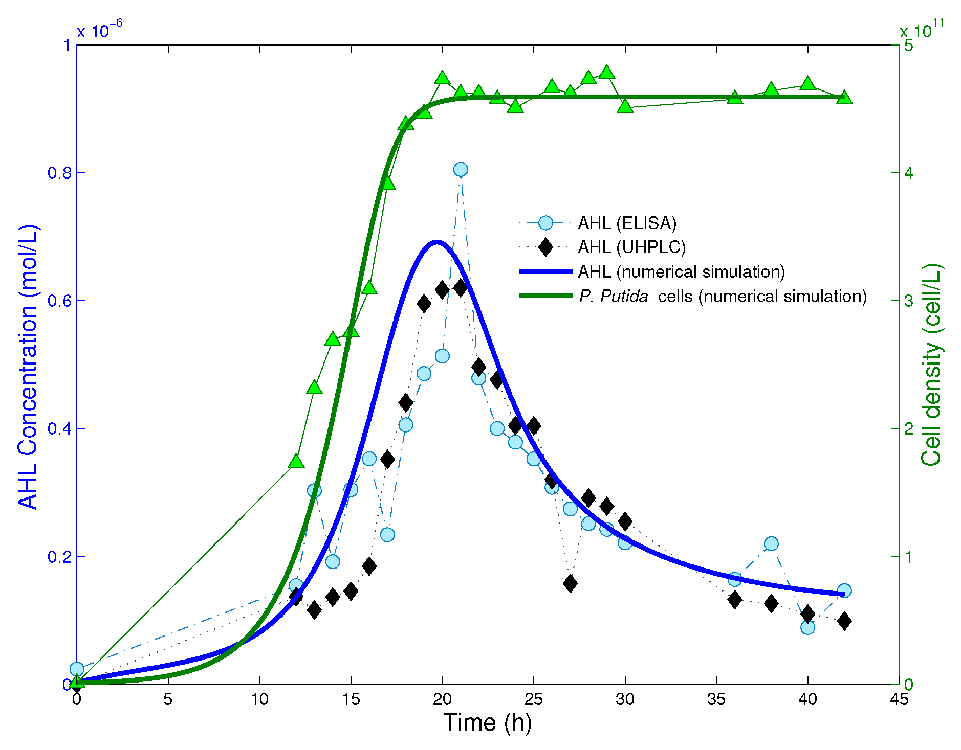
is the time at which bacteria have reached the saturation level. In Figure 2, we read from experimental data that the cell population reaches the equilibrium after ca. 20 h from the beginning of the experiment. Hence, we take t e c = 20 as the starting time point for numerical simulations of the reduced system (8), and define initial data on the time interval [ t e c - τ , t e c ] .
For simplicity, we assume that initial data are constant functions on the definition interval, see also [17,18]. We fix the value of the delay, τ = 2 h, as in [18]. Then we take x ( t ) = x ^ 19 , for t [ 18 , 20 ] , x ^ 19 being the mean value of ELISA and UHPLC measurements at 19 h from the beginning of the experiment. Initial data for the Lactonase are estimated from simulations of the full model (4) in [18]. To date, there is no experimental data available for Lactonase concentration, thus parameters associated with Lactonase production (ρ), decay (ω), and activity (δ) can be only estimated from AHL experimental data. This means in turn that there are several plausible solutions for the estimation of ρ , ω , and δ. We choose to maintain parameter values as estimated in [18].
It can be seen from the model reduction assumptions, as well as from the simplified parameters (7) that we lack information on the receptor production ( α R ) and decay ( γ R ); indeed, there is no equation for PpuR in (4). These parameters play a role for the critical threshold value, x t h , in the complex-regulated processes. We fit x t h and y ( t ) = y 0 , t [ 18 , 20 ] , fixing all other parameter values as in [18]. The results are summed up in 
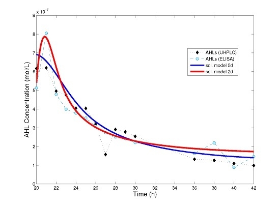
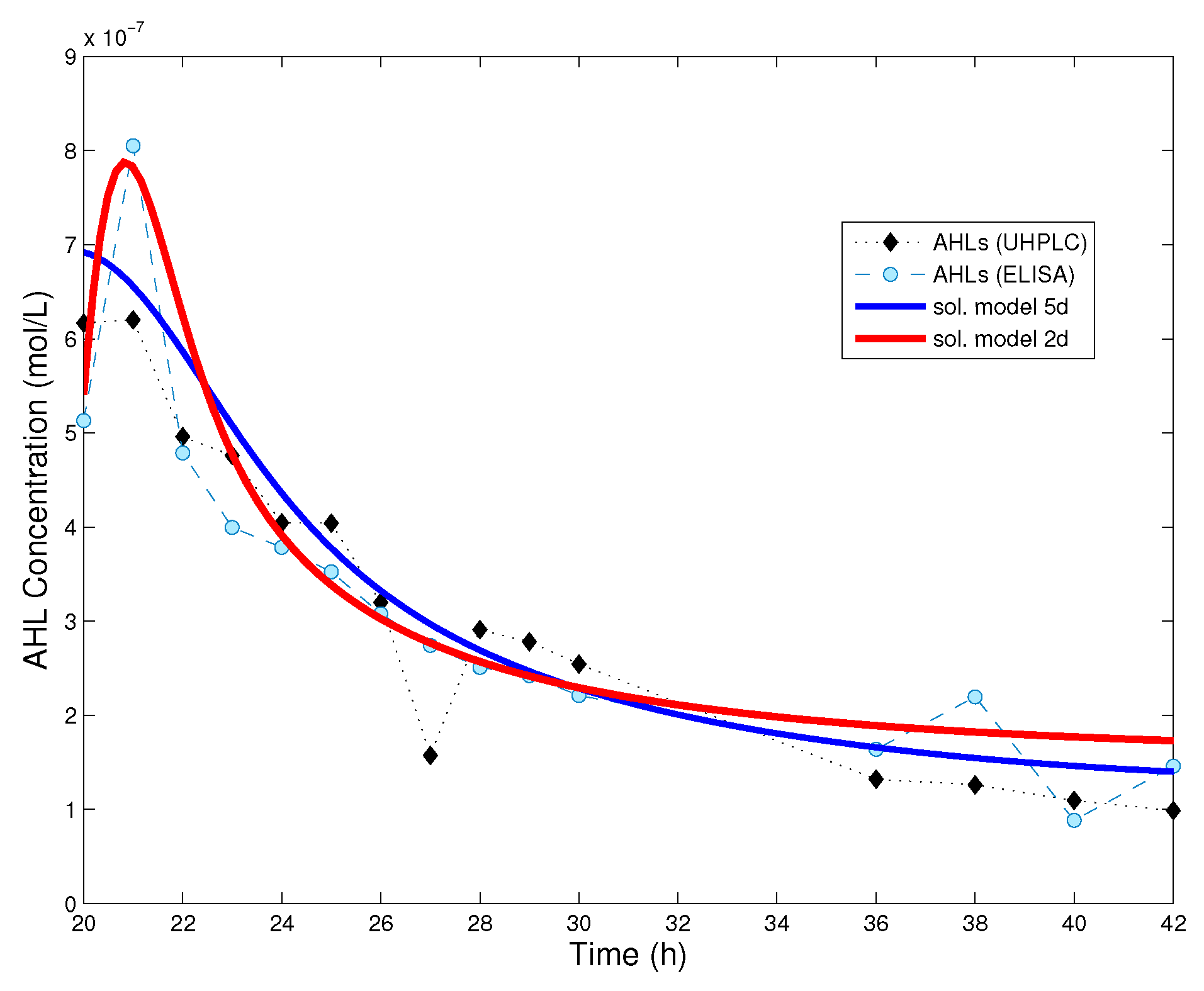
Table 1, with parameter values as provided by the fitting procedure, without rounding. In Figure 3 we show a comparison between the numerical solution of model (4), that of the simplified model (8) and experimental data for AHL time series.
With the estimated parameter values in Table 1, we consider the analytical results in Section 3.2 and Section 3.4. The system has three equilibrium points x ¯ 1 , x ¯ 2 , x ¯ 3 , but we only consider the stability properties of the largest one ( x 3 , y 3 ) = ( 1 . 593 × 10 - 7 , 4 . 809 × 10 4 ) , which corresponds to high AHL level and to an activated state of the bacteria population. Parameter values satisfy a 2 d 2 > b 2 c 2 , thus there is no stability switch with respect to τ, and the system behaves as in the case τ = 0 . We go back to Section 3.3 and consider the Jacobian matrix (13), obtaining t r ( J ) = - 7 . 4243 and det ( J ) = 0 . 7685 . Hence, with the estimated parameter values, the system (8) has a locally asymptotically stable equilibrium ( x 3 , y 3 ) in which bacteria are activated.

4. Discussion

In this paper we have introduced a system of two delay differential Equation (8) for quorum sensing of Pseudomonas putida in a continuous culture. Motivated by experimental data, a more detailed mathematical model (4) was previously proposed in [18]. Though the system (4) describes the regulatory network in greater detail, in the long run, bacteria reach a saturation level and the model can be reduced to two governing Equation (8), as we have shown in Section 2.1.
Surprisingly, even a simple model such as (8) can be used to explain experimental data (Figure 3), maintaining parameter values from a previous fit [18] for almost all model parameters. However, one should take into account that this is valid only from the moment the bacteria population has reached its saturation level. If one is interested in understanding quorum sensing in the initial phases (lag and exponential phase) of bacterial population, then it is convenient to use a more detailed model, such as (4) or (5).
The advantage of system (8) is that it can be investigated thoroughly thanks to well-established methods. We have shown existence and uniqueness of solutions and, more importantly, we could guarantee preservation of positivity. This property is often violated in systems of delay differential equations. We have studied linearized stability of non-negative equilibria and proved that the delay system (8) might show stability switches as the delay increases. On the other side, the Lactonase activity (δ) can induce Hopf-bifurcation in the associated ODE system (12).
For simplicity of computation in the analysis of the system, we have considered only the case of small Hill coefficients ( n = m = 2 ), which corresponds to a maximum of three biologically-relevant stationary states. This assumption is, however, not as restrictive as it seems. Three stationary states, with an intermediate unstable one, are the basis for the bistability situation already discovered in analogous regulatory networks [11,17]. Moreover, similar small values for the Hill coefficients were found to fit experimental data (Table 1) and correspond well to the biological assumption of a dimer being relevant for the positive feedback in the quorum sensing system of Pseudomonas putida [16]. With the fitted parameter values, we do not find delay-induced stability switches. This is not a hint of the delay being not relevant. Though a positive time lag might not change the main qualitative behavior of the system, the DDE model still describes the experimentally-determined data and their time course quantitatively better than the associated ODE system, in particular when the bacteria population is in the lag or exponential phase. Stability switches and periodic oscillatory behavior might appear for a different choice of the parameters in system (8). As the main focus of this work was to provide a description for a real biological process, we decided to omit further numerical investigation on the qualitative behavior of (8).
Delay equations have been previously used in mathematical models of continuous cultures. Commonly, a time lag was included to describe the time necessary for the bacteria to convert nutrients in new biomass [26,27]. Being interested in the long term dynamics with bacteria being at an equilibrium, we have chosen not to consider such reproduction lags in our model. In our case, the time lag arises from the dynamics of the regulatory network, in particular from the initialization processes of the AHL-degrading enzyme.
Taken together, the presented simplified delay equation system is a good compromise between refined modeling for a well-known gene regulatory network with several players, and a system of equations which still allows explicit analysis of the basic qualitative behavior as well as parameter determination from few experimental data.

Acknowledgments

Maria Vittoria Barbarossa is supported by the European Social Fund and by the Ministry of Science, Research and Arts Baden-Württemberg.

Author Contributions

M.V.B. and C.K. wrote the paper. M.V.B. collected and analyzed data. C.K. collected literature. M.V.B. and C.K. conceived the study. M.V.B. and C.K. developed the model. M.V.B. and C.K. performed model analysis. M.V.B. performed numerical simulations and parameter fitting.

Conflicts of Interest

The authors declare no conflict of interest.

References

  1. Nealson, K.H.; Platt, T.; Hastings, J.W. Cellular control of the synthesis and activity of the bacterial luminescent system. J. Bacteriol. 1970, 104, 313–322. [Google Scholar] [PubMed]
  2. Fuqua, W.C.; Winans, S.C.; Greenberg, E.P. Quorum sensing in bacteria: The LuxR-LuxI family of cell density-responsive transcriptional regulators. J. Bacteriol. 1994, 176, 269–275. [Google Scholar] [PubMed]
  3. Williams, P.; Winzer, K.; Chan, W.C.; Camara, M. Look who’s talking: Communication and quorum sensing in the bacterial world. Philos. Trans. R. Soc. Lond. Biol. 2007, 362, 1119–1134. [Google Scholar] [CrossRef] [PubMed]
  4. Yarwood, J.M.; Bartels, D.J.; Volper, E.M.; Greenberg, E.P. Quorum sensing in Staphylococcus aureus biofilms. J. Bacteriol. 2004, 186, 1838–1850. [Google Scholar] [CrossRef] [PubMed]
  5. Whitehead, N.; Barnard, A.; Slater, H.; Simpson, N.; Salmond, G. Quorum-sensing in Gram-negative bacteria. FEMS Microbiol. Rev. 2001, 25, 365–404. [Google Scholar] [CrossRef] [PubMed]
  6. Rumbaugha, K.; Griswold, J.; Hamood, A. The role of quorum sensing in the in vivo virulence of Pseudomonas aeruginosa. Microbes Infect. 2000, 2, 1721–1731. [Google Scholar] [CrossRef]
  7. Gustafsson, E.; Nilsson, P.; Karlsson, S.; Arvidson, S. Characterizing the dynamics of the quorum sensing system in Staphylococcus aureus. J. Mol. Microbiol. Biotechnol. 2004, 8, 232–242. [Google Scholar] [CrossRef] [PubMed]
  8. Cooley, M.; Chhabra, S.R.; Williams, P. N-Acylhomoserine lactone-mediated quorum sensing: A twist in the tail and a blow for host immunity. Chem. Biol. 2008, 15, 1141–1147. [Google Scholar] [CrossRef] [PubMed]
  9. Steidle, A.; Sigl, K.; Schuhegger, R.; Ihring, A.; Schmid, M.; Gantner, S.; Stoffels, M.; Riedel, K.; Givskov, M.; Hartmann, A.; et al. Visualization of N-acylhomoserine lactone-mediated cell-cell communication between bacteria colonizing the tomato rhizosphere. Appl. Environ. Microbiol. 2001, 67, 5761–5770. [Google Scholar] [CrossRef] [PubMed]
  10. Dockery, J.D.; Keener, J. A mathematical model for quorum sensing in Pseudomonas aeruginosa. Bull. Math. Biol. 2001, 63, 95–116. [Google Scholar] [CrossRef] [PubMed]
  11. Müller, J.; Kuttler, C.; Hense, B.A.; Rothballer, M.; Hartmann, A. Cell-cell communication by quorum sensing and dimension-reduction. J. Math. Biol. 2006, 53, 672–702. [Google Scholar] [CrossRef] [PubMed]
  12. Ward, J.; King, J.; Koerber, A.; Williams, P.; Croft, J.; Sockett, R. Mathematical modelling of quorum sensing in bacteria. Math Med. Biol. 2001, 18, 263–292. [Google Scholar] [CrossRef]
  13. Williams, J.; Cui, X.; Levchenko, A.; Stevens, A. Robust and sensitive control of a quorum-sensing circuit by two interlocked feedback loops. Mol. Syst. Biol. 2008, 4. [Google Scholar] [CrossRef] [PubMed]
  14. Jabbari, S.; King, J.; Koerber, A.; Williams, P. Mathematical modelling of the agr operon in Staphylococcus aureus. J. Math. Biol. 2010, 61, 17–54. [Google Scholar] [CrossRef] [PubMed]
  15. Koerber, A.; King, J.; Williams, P. Deterministic and stochastic modelling of endosome escape by Staphylococcus aureus: Quorum sensing by a single bacterium. J. Math. Biol. 2005, 50, 440–488. [Google Scholar] [CrossRef] [PubMed]
  16. Fekete, A.; Kuttler, C.; Rothballer, M.; Hense, B.A.; Fischer, D.; Buddrus-Schiemann, K.; Lucio, M.; Müller, J.; Schmitt-Kopplin, P.; Hartmann, A. Dynamic regulation of N-acyl-homoserine lactone production and degradation in Pseudomonas putida IsoF. FEMS Microbiol. Ecol. 2010, 72, 22–34. [Google Scholar] [CrossRef] [PubMed]
  17. Barbarossa, M.V.; Kuttler, C.; Fekete, A.; Rothballer, M. A delay model for quorum sensing of Pseudomonas putida. Biosystems 2010, 102, 148–156. [Google Scholar] [CrossRef] [PubMed]
  18. Buddrus-Schiemann, K.; Rieger, M.; Mühlbauer, M.; Barbarossa, M.V.; Kuttler, C.; Hense, A.B.; Rothballer, M.; Uhl, J.; Fonseca, J.R.; Schmitt-Kopplin, P.; et al. Analysis of N-acylhomoserine lactone dynamics in continuous cultures of Pseudomonas putida IsoF by use of ELISA and UHPLC/qTOF-MS-derived measurements and mathematical models. Anal. Bioanal. Chem. 2014, 406, 6373–6383. [Google Scholar] [CrossRef] [PubMed]
  19. Smith, H.L. An Introduction to Delay Differential Equations with Applications to the Life Sciences; Springer: New York, NY, USA, 2011. [Google Scholar]
  20. Goryachev, A.B.; Toh, D.J.; Lee, T. Systems analysis of a quorum sensing network: Design constraints imposed by the functional requirements, network topology and kinetic constants. Biosystems 2006, 83, 178–187. [Google Scholar] [CrossRef] [PubMed]
  21. Kuttler, C.; Hense, B.A. Interplay of two quorum sensing regulation systems of Vibrio fischeri. J. Theor. Biol. 2008, 251, 167–180. [Google Scholar] [CrossRef] [PubMed]
  22. Pearson, J.P.; van Delden, C.; Iglewski, B. Active efflux and diffusion are involved in transport or Pseudomonas aeruginosa cell-to-cell signals. J. Bacteriol. 1999, 181, 1203–1210. [Google Scholar] [PubMed]
  23. Smith, H.L.; Waltman, P. The Theory of the Chemostat: Dynamics of Microbial Competition; Cambridge University Press: Cambridge, UK, 1995; Volume 13. [Google Scholar]
  24. Kuang, Y. Delay Differential Equations: With Applications in Population Dynamics; Academic Press: Cambridge, MA, USA, 1993. [Google Scholar]
  25. Bellen, A.; Zennaro, M. Numerical Methods for Delay Differential Equations; Oxford University Press: Oxford, UK, 2013. [Google Scholar]
  26. Ellermeyer, S.F. Competition in the chemostat: Global asymptotic behavior of a model with delayed response in growth. SIAM J. Appl. Math. 1994, 54, 456–465. [Google Scholar] [CrossRef]
  27. Freedman, H.I.; So, J.W.H.; Waltman, P. Coexistence in a model of competition in the chemostat incorporating discrete delays. SIAM J. Appl. Math. 1989, 49, 859–870. [Google Scholar] [CrossRef]
Figure 1. Model structure for the quorum sensing system in one Pseudomonas putida cell. N-Acyl homoserine lactone (AHL) concentration is regulated by a (self-induced) positive feedback (+) as well as by a negative feedback (−) via the AHL-degrading enzyme Lactonase. The transcriptional activator PpuR binds to AHL forming a PpuR–AHL complex, which polymerizes. PpuR–AHL n-mers bind to the AHL-dependent quorum sensing locus (ppu-box) and synthesize PpuI. This protein is finally responsible for AHL synthesis. Similarly, PpuR-AHL n-mers induce synthesis of Lactonase molecules. Feedbacks on the transcription of PpuR are neglected. Solid arrows represent activations and inhibitions. Dashed arrows indicate reactions and processes which are partially assumed to be in quasi-steady state. Dotted arrows represent the possible exchange of substances between intracellular and extracellular space. The dashed green ellipse refers to the special case in model version (4), where it is assumed that the total amount of PpuR in one cell (consisting of PpuR and the PpuR-AHL complex) is constant whereas in the other models, PpuR and the PpuR-AHL complex follow their own dynamics.
Applsci 06 00149 g001
Figure 2. Experimental data and numerical solution of the mathematical model (4). Picture adapted from [18]. Copyright 2014, Springer-Verlag Berlin Heidelberg. The cell population reaches its equilibrium after approximatively 20 h from the beginning of the experiment.
Applsci 06 00149 g002
Figure 3. Comparison between the numerical solution of the dynamical systems and experimental data. Red curve: solution of the reduced system (8); Blue curve: solution of the full model (4) in [18]. Initial data for the reduced system are x ( t ) = x 0 ( t ) , y ( t ) = y 0 ( t ) , t [ 18 , 20 ] , where y 0 ( t ) 5 . 2 × 10 - 13 was fitted and x 0 ( t ) 5 . 4044 × 10 - 7 is the mean value of ELISA and UHPLC measurements at 19 h from the beginning of the experiment. When the cell population has reached its stationary level, the reduced model provides a good approximation of the dynamics. Parameter values used for the reduced model are given in Table 1.
Applsci 06 00149 g003
Table 1. Variables and parameters in model (8), with values used for data fit in Figure 3.
SymbolDescriptionValue (Unit)Comments/Source
N * Cell density at equilibrium 4 . 5929 × 10 11 (cells/lit)[18]
αBasic AHL production rate 1 . 0564 × 10 - 7 (mol/(lit 2 · h)) = α A * N e q u i , [18]
γAHL decay rate (includes washout)0.105 (1/h) = γ A + D , [18]
δLactonase-dependent degradation rate 1 . 5000 × 10 - 4 (lit/(mol · h))[18]
βFeedback-regulated AHL production rate 1 . 0564 × 10 - 6 (mol/(lit 2 · h)) = β A * N e q u i , [18]
nHill coefficient for x2.3 (dimensionless)[18]
x t h Critical threshold for positive-feedback in x 3 . 597 × 10 - 13 (mol/lit)estimated
ωLactonase decay rate (includes washout)0.105 (1/h) = γ e + D , [18]
ρLactonase production rate 5 . 0521 × 10 3 (mol/(lit 2 · h)) = α e * N e q u i , [18]
τDelay in the release of y2 (h)[18]
mHill coefficient for x2.5 (dimensionless)[18]
y t h Critical threshold for positive-feedback in y 3 . 597 × 10 - 13 (mol/lit)estimated
x 0 ( t ) AHL concentration (initial data) t [ 18 , 20 ] 5 . 4044 × 10 - 7 (mol/lit)mean of exp. data
y 0 ( t ) Lactonase (initial data) t [ 18 , 20 ] 5 . 2 × 10 3 (mol/lit)estimated

