Multivariate Analysis of Transient State Infrared Images in Production Line Quality Control Systems


1
Department of Research for Innovation, Loccioni Group, via Fiume 16, 60030 Angeli di Rosora, Italy
2
Faculty of Electrical Engineering, Silesian University of Technology, ul. Akademicka 10, 44-100 Gliwice, Poland
*
Author to whom correspondence should be addressed.
Appl. Sci. 2018, 8(2), 250; https://0-doi-org.brum.beds.ac.uk/10.3390/app8020250
Submission received: 15 December 2017
/
Revised: 2 February 2018
/
Accepted: 4 February 2018
/
Published: 7 February 2018
(This article belongs to the Special Issue Novel Ideas for Infrared Thermography also Applied in Integrated Approaches)
Abstract
:Manufacturers would like to increase production volumes while preserving the high quality of their products. The long testing times can cause a bottleneck of production processes especially taking into account the observed tendency for testing all produced devices. The main aim of this work consists in the analysis of time changes of features extracted from thermal images using the multivariate approach. The paper shows that if the principal component analysis (PCA), belonging to multivariate methods, is applied for quality control based on infrared images, then the minimum testing times can be estimated. In order to draw the final conclusions regarding testing times and, what is also very important, which principal components should be selected for classification, a detailed temporal analysis for an exemplary production line has been carried out. The future impact of the results includes higher productivity and cost-effectiveness due to the determination of an optimal decision time in production line quality control systems using the proposed approach.
1. Introduction
The constant development of measuring techniques and equipment results in a huge amount of data available for quality control tasks. Thermal imaging and thermal cameras are very good examples of this trend [1]. However, the progress in hardware capabilities would be useless if not followed by the progress in algorithms and software [2,3]. Of course, new algorithms force hardware development, too. In general, both key players in quality control, i.e., hardware and software, influence each other.
A pattern recognition system used for industrial quality control based on infrared images has to be highly reliable and fast. While the reliability is a self-evident feature of any system aimed at industry, the acceptable time for testing a single device is highly dependent on the application. Sometimes the algorithm that is too slow for the production line application gives the most accurate results. Therefore, especially in the case of very high-volume production lines, the choice of the algorithm should be a compromise between the classification reliability and speed of calculation.
This paper is devoted to the application of a well-known multivariate algorithm, i.e., PCA, to analysis of data acquired with the help of thermal cameras. The successful application of such algorithms in other fields allows us to expect improvement of production line quality control results. Multivariate algorithms enable reduction of the dimension of input space in classification problems and so they make them easier to solve [4]. It is especially important in the case of n × m images for which each pixel can be treated as a separate piece of information, and so the dimension of the input space can be as high as n × m [5]. Depending on the resolution, information included in adjacent pixels can be more or less correlated and feature extraction is indispensable [6].
Quality control can be based on single thermal images (2D data) but the output signal of a thermal camera is a 3D signal. In this paper, the importance of the third dimension through detailed analysis of the time evolution of features extracted using a multivariate algorithm has been shown. Such an approach, i.e., temporal analysis of PCA results aimed at acquisition time selection, has not been presented in the literature. The current state of the art of applications of PCA in infrared imaging has been presented in Section 3. So far, the testing time has been selected on the base of temporal thermal contrast evolution [7]. Some rough estimations have been also used to set the acquisition time which should be optimal to perform quality control [8,9,10]. However, such estimations usually suffer from overestimating the required time which is especially undesirable in production line applications. Moreover, this research has revealed that in some cases waiting too long can decrease the efficiency of the quality control based on thermal images.
Transient state analysis of thermal images has been considered in many papers. In the simplest case the feature extraction has not been applied and each pixel of the thermal image has been used for classification [5,10,11]—the comparison of heating and cooling patterns for each pixel or the number of pixels above a threshold value allows for the detection of elements or regions with defects. Sometimes it is enough to monitor time changes of maximum temperature. Advanced temporal analysis, but not based on a multivariate approach, can be found in [2]—the classification is based on time waveforms representing statistical features extracted from the fused infrared and vision images. The other application of infrared temporal analysis consists in the calculation of energy balance and heating curves of electrical machines which afterwards can be used for defect detection [12]. The temperature time history of the thermographic data is also used to extract the region of interest before applying post-processing and classification methods [13].
This paper aims at bringing advanced data analysis techniques based on multivariate approach to thermal image processing. The novelty of the paper consists in the detailed analysis of principal components temporal behavior aimed at the selection of the components which ensure the shortest time for performing production line quality control. The main conclusion is that it is possible to minimize the time required for quality control and obtain satisfactory quality control results but the principal components selection must be made individually for each problem. These factors, i.e., time and quality, are crucial in production line applications of infrared imaging.
The PCA, as a well-established method, has been briefly described in the following section and next its application to analysis of infrared images has been given.
2. Fundamentals of Principal Component Analysis
The contemporary real-world systems become more and more complicated so one needs more and more variables to describe it. A set of these variables is just a point in the measurement space. If the dimension of this space is high then methods of its reduction become very important as they simplify the analysis, help to uncover the relationship between observations and variables revealing groups or trends and enable visualization of the data. PCA is one of these methods. It consists in the projection of the data into space in which the first axis of the new coordinate system is aligned with the direction where the data has the largest variance. The next axes are ordered according to the value of variance of the data for the direction they represent. Moreover, this principal coordinate system is orthogonal. From the mathematical point of view the original coordinate system and principal coordinate system are related by an affine transform, i.e., translation and rotation. So PCA is a statistical procedure that performs a linear subspace projection. It enables data compression while preserving the major features of the data. PCA involves minimization of the mean square error between the projected data (onto an m-dimensional subspace) and the original data (given for the n-dimensional space, n > m).
The PCA is based on the following theorem of linear algebra [4]. If an n-dimensional vector x has the covariance matrix Cx, then there exists an orthogonal transform:
such that the covariance matrix Cy of the vector y is:
where λ1 ≥ λ2 ≥ … ≥ λn are the eigenvalues of the matrix Cx and the columns of Q are the corresponding eigenvectors.
The components of y are statistically uncorrelated. Moreover, each component has the maximum variance among all normalized linear combinations that are uncorrelated with the other components. It can therefore be said that y is the vector of principal components of x and the method is called PCA.
The projection of the data onto a smaller dimensionality space m (m < n) is commonly called feature extraction. What is important, such projection always results in data distortion. The error of approximation of the data set by only m features is equal to the sum of the eigenvalues that have not been taken into account:
Principal components (PCs) can be calculated not only with the help of classical algorithms based on eigenvector calculation, but also by means of more sophisticated ones like Karhunen–Loeve transform or neural networks. One can use also Singular Value Decomposition (SVD) which allows us to express a given m-by-n real matrix A, with m > n, as:
where U and VT are orthogonal matrices, So is n-by-n diagonal matrix with elements on the diagonal in decreasing order. These elements are called singular values of the matrix A. The time of calculation is the main drawback of using SVD to calculate PCs in the case of high dimensional spaces. Moreover, usually only the first few PCs are important and SVD calculates all n PCs. A method that enables us to determine only PCs that are needed is called the deflation method. It resembles the well-known recursive orthogonalization procedure by Gram–Schmidt.
3. Application of PCA to Infrared Image Analysis in Production Line Quality Control Systems
Data mining that leads to information extracting is one of the biggest challenges of contemporary science and one of the main needs of modern industry. In many present-day applications the problem is not to get the data but to analyze a huge amount of easily accessible information in order to make some decisions. Multivariate methods are a tool that can be used to solve this problem. Thermal image analysis belongs to this group of applications for which multivariate methods, including PCA, can be very useful. They become more and more popular in other fields and for sure they deserve also more attention from the infrared community.
It must be stressed that the effectiveness of PCA in the solution of a particular problem should always be verified. There is no guarantee that classifiers based on PCA features will work well, because PCA determines the projection of the data that enables the best reconstruction and not necessarily the best classification. So far PCA of infrared images has been used for non-destructive testing of materials [14,15,16,17]. It is especially useful for data compression in non-destructive examination and an IR-video sequence and what follows the reduction of processing times required for image classification [18,19,20]. However, there are almost no references on the application of PCA approach to high volume production line quality control [6]. Recently, application of the Candid Covariance-Free Incremental Principal Component Thermography (CCIPCT) as well as the Sparse Principal Component Analysis (SPCA) based K-means clustering for automatic defect segmentation in infrared non-destructive testing have been proposed [21,22]. The CCIPCT method is an extension of Principal Component Thermography (PCT) which has been proposed as a method for defect depth characterization [23,24]. The other relatively new PCA application consists in the enhancement of contrast [25] and removal of the noise and information redundancy of the infrared image sequences [26].
The transformation of the original thermal images into principal components applied in production line quality control has been illustrated in Figure 1. The detailed description of the procedure and the classification algorithm have been given in [6]. In this paper, analysis and discussion of time evolution and selection of principal components is a key problem.
The analysis of temporal evolution of principal components aimed at the optimization of production line quality control for home appliances has been carried out taking refrigerators as a device under test (DUT). They can be regarded as complex units exhibiting a dynamic thermal process after switching on. Although the first question was how to set the time of inspection in order to get the best quality control results, the performed analysis have led us to answers regarding some other questions and more general recommendations valid when dealing with PCA in such application [6]. A typical layout of the production line quality control system based on infrared imaging has been presented in Figure 2.
If infrared images have the resolution of 320 × 240 pixels then the input feature space is 76800-dimensional assuming that each pixel is an input variable. The reduction of the dimension of the feature space to 2D presented by Grabowski and Cristalli [6] allowed for fast classification and simple interpretation and visualization of classification results. Of course, it brings about loss of information, which can be accepted as long as the correct classification is possible.
4. Temporal Evolution of Principal Components in Exemplary Production Line Application
The first question that must be addressed is how to set the shortest image acquisition time which ensures a good discrimination between fully functional and faulty devices. In the case of refrigerators, the transient thermal state which takes place after switching on takes a few minutes, usually not more than 10–15 min. The heating process has been illustrated in Figure 3 which shows typical time changes of evaporator inlet and outlet average temperatures. What is the shortest time after which quality control can be carried out using PCA approach?
Let us conduct PCA analysis for 10 devices including 5 defective devices belonging to class B (red and empty point curves in Figure 4, Figure 5 and Figure 6) and 5 non-defective devices belonging to class G (green and filled point curves in Figure 4, Figure 5 and Figure 6). The time dependence of the first 2 PCs has been shown in Figure 4 and Figure 5. The answer to the question asked in the beginning of this section can be given. In this example the minimum image acquisition time should be set to 5 min.
It must be noticed that behavior of PCs is different—the discrimination between classes for PC1 remains, while for PC2 it reduces significantly after 10 min and practically declines after 12 min. It is also visible in Figure 6 which includes data clusters obtained after 17 min. In order to get the best separation between classes the acquisition time should be set to 8 min.
The results presented in Figure 4, Figure 5 and Figure 6 could suggest that the first two PCs, representing the most of the total variance of the data, should be used for quality control. Unfortunately, such theorem is not true. The following example concerning the same type of device but a different model shows that selection of PCs must be made very carefully and separately for each model. In this case, there are 21 devices under consideration including:
For a defective refrigerator of class E (Figure 7b), the evaporator outlet temperature is higher than in the case of non-defective devices (Figure 7a). It means that the evaporator is not working properly. For a defective refrigerator of class B (Figure 7c), the temperature difference between the evaporator inlet and outlet is higher than usual. It can be caused by an occlusion, an overcharge or undercharge of liquid refrigerant. Generally, the correct classification of devices that belong to class E is not an easy task but it is usually possible as it has been shown below.
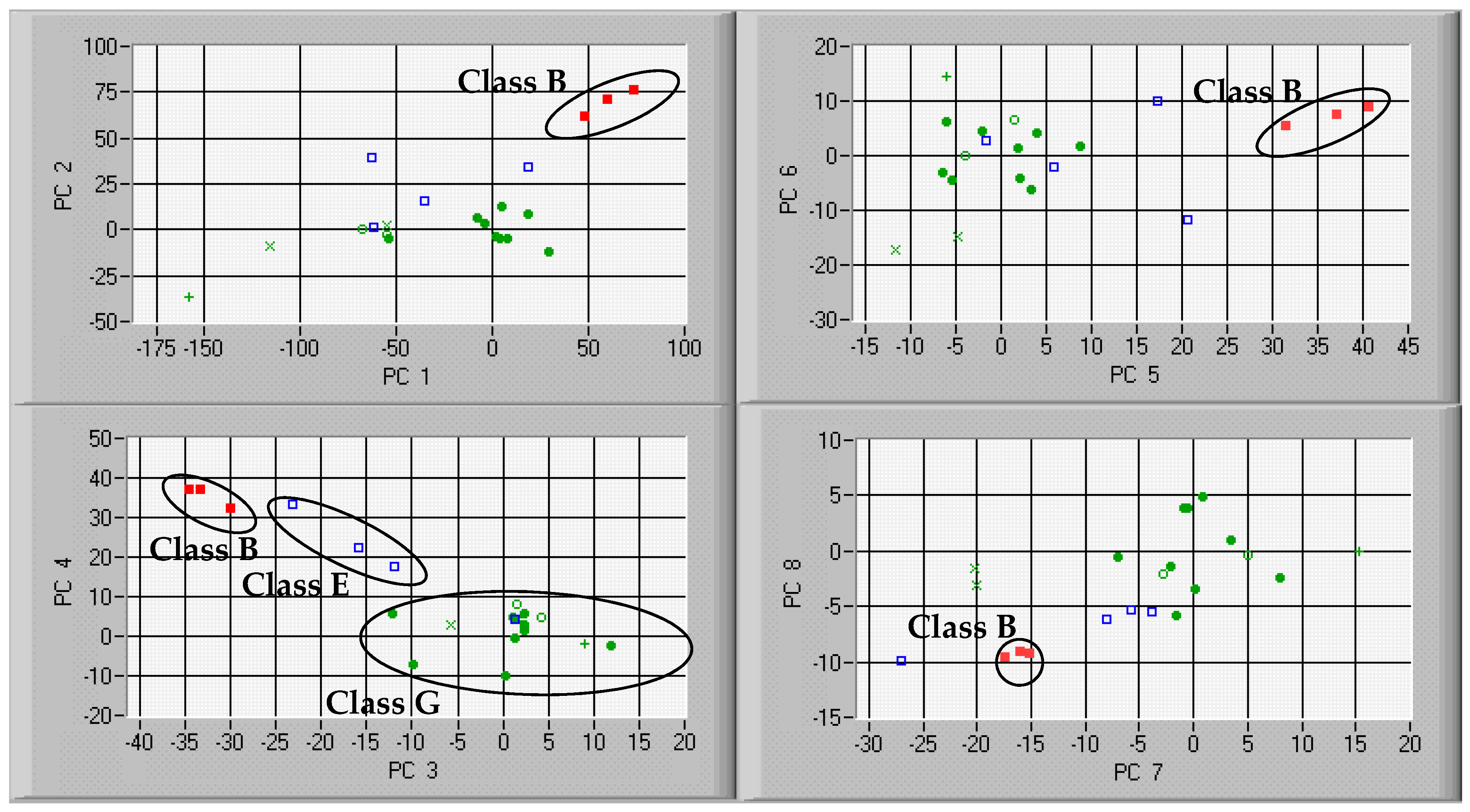
The analysis of Figure 8, Figure 9, Figure 10, Figure 11 and Figure 12 leads to a conclusion that the classification using PC1 and PC2 is possible in this case but it requires much longer acquisition time (Figure 12), which in the production line environment can be unacceptable. Moreover, the comparison between PCs presented in Figure 11 results in a conclusion that for this acquisition time it is better to choose PC2 and PC5 in order to obtain higher class separation. Successive plots in Figure 8, Figure 9, Figure 10, Figure 11 and Figure 12 have axes being successive PCs. Of course, the best PCs for classification are not always consecutive, e.g., PC2 and PC5 for the time of acquisition equal to 15 min.
It is evident that in this example PC3 and PC4 are the only components that enable quick classification after just 4 min (Figure 8). On the other hand, the separation between classes for these PCs decreases with time (Figure 9, Figure 10 and Figure 11) and they do not allow us to perform reliable classification for times greater than 10 min (Figure 12).
The classification can be made after about 5 min depending on the device model. It is two times less than the time indicated in some other publications [8,9]. Moreover, tests proved that it is even easier to detect some faults, e.g., evaporator defects (class E, Figure 8, Figure 9, Figure 10, Figure 11 and Figure 12), on the base of infrared images taken during the transient state (for times less than 10 min).
As for the classification efficiency, the analysis of Figure 8, Figure 9, Figure 10, Figure 11 and Figure 12 reveals that one of the faulty devices belonging to class E cannot be correctly classified using PCA approach. It must be noticed that its infrared image, presented in Figure 7b, is very similar to the image of a non-defective device presented in Figure 7a. Therefore, the final efficiency is equal to 95.2%.
In Figure 8, Figure 9, Figure 10, Figure 11 and Figure 12, it can be noticed that class B can be separated for almost all PCs and all acquisition times—in 18 considered cases out of 20 comparing to 6 for the class G and E assuming acceptable level of classification efficiency to be equal at least 95%.
As it has been already suggested, it is not possible to point out the best PCs before performing a preliminary analysis of the data. Table 1 shows the time dependence of the total variance of data covered by each PC. Can it be helpful to choose the best PCs?
In order to answer this question, the relative changes of total variance values covered by each PC have been presented in Figure 13. It has been assumed that the PC total variance values for t = 240 s are reference values. Two groups of PCs can be distinguished. The first group, for which the relative value changes are less than ±15%, includes PC1, PC4, PC5 and PC7. The second group, for which the relative value changes are higher than +25% and less than +55%, includes PC2, PC3, PC6 and PC8. The variance for the PC1 is decreasing with time when the other values are non-monotonically increasing (PC2–PC3 and PC5–PC8) or stay at the same level (PC4). Two PCs with the best classification power for each acquisition time have been indicated by yellow background in Figure 13. It seems that there is no simple rule that could be used to select PCs for classification on the base of the time dependence of the variance for each PC.
5. Conclusions
It is possible to reduce testing times and so the unit costs of production line quality control, which are proportional to the testing times, by application of the infrared imaging and the principal component analysis. Tests performed during the thermal transient state can simplify classification of devices with defects difficult or even impossible to be detected in the steady state using PCA approach. As for the transient state dynamics, the time constants as well as initial and steady state values are different for each PC—the waveforms describing the time behavior of the PCs can be approximated by solutions of ordinary linear differential equations of the second order with constant coefficients. However, there is no algorithm which allows us to select the best PCs in advance—each case must be considered individually.
Future research directions may include application of self-organizing neural networks for clustering the PCA results especially if more than two principal components must be chosen to reach the required classification efficiency level. Such an approach will enable easy and understandable presentation of the data clusters as it is possible to visualize high-dimensional input spaces in two dimensions of the network topology. The performance of some other classifiers, such as support vector machines or decision trees combined with the AdaBoost algorithm, can be also verified and compared.
Acknowledgments
This work was partly supported by the EU under the project number G1TR-CT-2000-00030.
Author Contributions
Cristina Cristalli conceived, designed and performed the experiments; Dariusz Grabowski analyzed the data; Cristina Cristalli contributed analysis tools; Cristina Cristalli and Dariusz Grabowski wrote the paper.
Conflicts of Interest
The authors declare no conflict of interest.
References
- Vollmer, M.; Mollmann, K.P. Infrared Thermal Imaging: Fundamentals, Research and Applications; Wiley–VCH Verlag GmbH & Co. KGaA: Weinheim, Germany, 2010; ISBN 9783527407170. [Google Scholar]
- Fidali, M.; Jamrozik, W. Diagnostic method of welding process based on fused infrared and vision images. Infrared Phys. Technol. 2013, 61, 241–253. [Google Scholar] [CrossRef]
- Glowacz, A.; Glowacz, Z. Diagnosis of the three-phase induction motor using thermal imaging. Infrared Phys. Technol. 2017, 81, 7–16. [Google Scholar] [CrossRef]
- Rencher, A.C.; Christensen, W.F. Methods of Multivariate Analysis, 3rd ed.; John Wiley & Sons Inc.: Hoboken, NJ, USA, 2012; ISBN 9780470178966. [Google Scholar]
- González, D.A.; Madruga, F.J.; Quintela, M.Á.; López -Higuera, J.M. Quality control of radiant heaters. Proc. SPIE Photonics Appl. Ind. Res. IV 2015, 5948, 594823. [Google Scholar] [CrossRef]
- Grabowski, D.; Cristalli, C. Production line quality control using infrared imaging. Infrared Phys. Technol. 2015, 71, 416–423. [Google Scholar] [CrossRef]
- Legrand, A.-C.; Meriaudeau, F.; Gorria, P. Active infrared non-destructive testing for glue occlusion detection within plastic lids. NDT E Int. 2002, 35, 177–187. [Google Scholar] [CrossRef]
- Cristalli, C.; de Grassi, A.; Rodriguez, R.M. A Fast on Line Quality Control of Refrigerators Based on Thermal Image Detection and Power Consumption. In Proceedings of the International Refrigeration and Air Conditioning Conference, Purdue, IN, USA, 16–19 July 2002; p. 614. [Google Scholar]
- Björk, E.; Palm, B.; Nordenberg, J. A thermographic study of the on–off behavior of an all-refrigerator. Appl. Therm. Eng. 2010, 30, 1974–1984. [Google Scholar] [CrossRef]
- Liu, F.; Yang, S.; Leng, C.; Su, Z. Simulation on quantitative analysis of crack inspection by using eddy current stimulated thermography. In Proceedings of the Far East Forum on Nondestructive Evaluation/Testing: New Technology & Application (FENDT), Jinan, China, 17–20 June 2013; pp. 59–64. [Google Scholar] [CrossRef]
- Meola, C.; Carlomagno, G.M. Infrared thermography to evaluate impact damage in glass/epoxy with manufacturing defects. Int. J. Impact Eng. 2014, 67, 1–11. [Google Scholar] [CrossRef]
- Picazo-Ródenas, M.J.; Royo, R.; Antonino-Daviu, J.; Roger-Folch, J. Use of infrared thermography for computation of heating curves and preliminary failure detection in induction motors. In Proceedings of the XX International Conference on Electrical Machines (ICEM), Marseille, France, 2–5 September 2012; pp. 525–531. [Google Scholar] [CrossRef]
- Usamentiaga, R.; Venegas, P.; Guerediaga, J.; Vega, L.; López, I. Feature extraction and analysis for automatic characterization of impact damage in carbon fiber composites using active thermography. NDT E Int. 2013, 54, 123–132. [Google Scholar] [CrossRef]
- Cheng, L.; Tian, G.Y. Transient thermal behavior of eddy-current pulsed thermography for nondestructive evaluation of composites. IEEE Trans. Instrum. Meas. 2013, 62, 1215–1222. [Google Scholar] [CrossRef]
- Bendada, A.; Sfarra, S.; Genest, M.; Paoletti, D.; Rott, S.; Talmy, E.; Ibarra-Castanedo, C.; Maldague, X. How to reveal subsurface defects in Kevlar® composite materials after an impact loading using infrared vision and optical NDT techniques? Eng. Fract. Mech. 2013, 108, 195–208. [Google Scholar] [CrossRef]
- Cheng, L.; Gao, B.; Tian, G.Y.; Woo, W.L.; Berthiau, G. Impact damage detection and identification using eddy current pulsed thermography through integration of PCA and ICA. IEEE Sens. J. 2014, 14, 1655–1663. [Google Scholar] [CrossRef]
- Griefahn, D.; Wollnack, J.; Hintze, W. Principal component analysis for fast and automated thermographic inspection of internal structures in sandwich parts. J. Sens. Sens. Syst. 2014, 3, 105–111. [Google Scholar] [CrossRef]
- Winfree, W.P.; Cramer, K.E.; Zalameda, J.N.; Howell, P.A.; Burke, E.R. Principal component analysis of thermographic data. In Thermosense: Thermal Infrared Applications XXXVII; International Society for Optics and Photonics: Washington, DC, USA, 2015; Volume 9485, p. 94850S. [Google Scholar] [CrossRef]
- Świta, R.; Suszyński, Z. Processing of thermographic sequence using Principal Component Analysis. Meas. Autom. Monit. 2015, 61, 215–218. [Google Scholar]
- Marinetti, S.; Grinzato, E.; Bison, P.G.; Bozzi, E.; Chimenti, M.; Pieri, G.; Salvetti, O. Statistical analysis of IR thermographic sequences by PCA. Infrared Phys. Technol. 2004, 46, 85–91. [Google Scholar] [CrossRef]
- Yousefi, B.; Sfarra, S.; Ibarra-Castanedo, C.; Maldague, X.P.V. Comparative analysis on thermal non-destructive testing imagery applying Candid Covariance-Free Incremental Principal Component Thermography (CCIPCT). Infrared Phys. Technol. 2017, 85, 163–169. [Google Scholar] [CrossRef]
- Yousefi, B.; Sharifipour, H.M.; Ibarra-Castanedo, C.; Maldague, X.P.V. Automatic IRNDT inspection applying sparse PCA-based clustering. In Proceedings of the IEEE 30th Canadian Conference on Electrical and Computer Engineering (CCECE), Windsor, ON, Canada, 30 April–3 May 2017; pp. 1–4. [Google Scholar] [CrossRef]
- Rajic, N. Principal component thermography for flaw contrast enhancement and flaw depth characterisation in composite structures. Compos. Struct. 2002, 58, 521–528. [Google Scholar] [CrossRef]
- Omar, M.A.; Parvataneni, R.; Zhou, Y. A combined approach of self-referencing and Principle Component Thermography for transient, steady, and selective heating scenarios. Infrared Phys. Technol. 2010, 53, 358–362. [Google Scholar] [CrossRef]
- Wei, W.; Wei, L.; Nie, L.; Su, L.; Lu, X. Using active thermography and modified SVM for intelligent diagnosis of solder bumps. Infrared Phys. Technol. 2015, 72, 163–169. [Google Scholar] [CrossRef]
- Tang, Q.; Bu, C.; Liu, Y.; Qi, L.; Yu, Z. A new signal processing algorithm of pulsed infrared thermography. Infrared Phys. Technol. 2015, 68, 173–178. [Google Scholar] [CrossRef]
Figure 1.
Block diagram of the quality control principal component analysis (PCA)-based algorithm and data at its successive steps. PCs: Principal components.
Figure 1.
Block diagram of the quality control principal component analysis (PCA)-based algorithm and data at its successive steps. PCs: Principal components.

Figure 2.
Exemplary production line quality control system with a device under test (DUT) inspected with the help of an infrared camera (IR)—sources of radiation received by the camera have been presented.
Figure 2.
Exemplary production line quality control system with a device under test (DUT) inspected with the help of an infrared camera (IR)—sources of radiation received by the camera have been presented.

Figure 3.
Time evolution of evaporator inlet and outlet average temperatures.

Figure 4.
Time dependence of the first principal component (PC1) of thermal images (10 devices).

Figure 5.
Time dependence of the second principal component (PC2) of thermal images (10 devices).

Figure 6.
Time evolution of infrared images illustrated in 2D feature space composed of PC1 and PC2.
Figure 6.
Time evolution of infrared images illustrated in 2D feature space composed of PC1 and PC2.

Figure 7.
Exemplary infrared images of devices belonging to: (a) class G—non-defective devices; (b) class E—defective devices with faulty evaporator; (c) class B—defective devices with other than evaporator faults.
Figure 7.
Exemplary infrared images of devices belonging to: (a) class G—non-defective devices; (b) class E—defective devices with faulty evaporator; (c) class B—defective devices with other than evaporator faults.

Figure 8.
Representation of devices by PC1–PC8 for acquisition time equal to 4 min.

Figure 9.
Representation of devices by PC1–PC8 for acquisition time equal to 5 min.

Figure 10.
Representation of devices by PC1–PC8 for acquisition time equal to 7.5 min.

Figure 11.
Representation of devices by PC1–PC8 for acquisition time equal to 10 min.

Figure 12.
Representation of devices by PC1–PC8 for acquisition time equal to 15 min.

Figure 13.
Relative changes of total variance for PC1–PC8 as functions of the acquisition time.


Table 1.
Percentage of total variance of data covered by principal components calculated for different measurement times.
Table 1.
Percentage of total variance of data covered by principal components calculated for different measurement times.
| Principal | Percentage of Total Variance of Data Covered by Principal Components (%) | ||||
|---|---|---|---|---|---|
| Component | t = 240 s | t = 300 s | t = 450 s | t = 600 s | t = 900 s |
| PC1 | 75.4 | 73.6 | 70.6 | 70.0 | 68.1 |
| PC2 | 6.5 | 6.8 | 8.5 | 8.8 | 9.9 |
| PC3 | 5.0 | 5.6 | 6.6 | 7.3 | 7.1 |
| PC4 | 4.2 | 4.5 | 4.1 | 4.3 | 4.2 |
| PC5 | 3.2 | 3.2 | 3.6 | 3.2 | 3.6 |
| PC6 | 2.2 | 2.6 | 2.7 | 2.8 | 3.0 |
| PC7 | 2.1 | 2.2 | 2.2 | 1.8 | 2.4 |
| PC8 | 1.4 | 1.5 | 1.8 | 1.7 | 1.8 |
| PC9-768 | 0.0 | 0.0 | 0.0 | 0.0 | 0.0 |
© 2018 by the authors. Licensee MDPI, Basel, Switzerland. This article is an open access article distributed under the terms and conditions of the Creative Commons Attribution (CC BY) license (http://creativecommons.org/licenses/by/4.0/).
Share and Cite
MDPI and ACS Style
Cristalli, C.; Grabowski, D. Multivariate Analysis of Transient State Infrared Images in Production Line Quality Control Systems. Appl. Sci. 2018, 8, 250. https://0-doi-org.brum.beds.ac.uk/10.3390/app8020250
AMA Style
Cristalli C, Grabowski D. Multivariate Analysis of Transient State Infrared Images in Production Line Quality Control Systems. Applied Sciences. 2018; 8(2):250. https://0-doi-org.brum.beds.ac.uk/10.3390/app8020250
Chicago/Turabian StyleCristalli, Cristina, and Dariusz Grabowski. 2018. "Multivariate Analysis of Transient State Infrared Images in Production Line Quality Control Systems" Applied Sciences 8, no. 2: 250. https://0-doi-org.brum.beds.ac.uk/10.3390/app8020250
Note that from the first issue of 2016, this journal uses article numbers instead of page numbers. See further details here.