Constraint-Based Time-Scale Modification of Music Recordings for Noise Beautification

Abstract

In magnetic resonance imaging (MRI), a patient is exposed to beat-like knocking sounds, often interrupted by periods of silence, which are caused by pulsing currents of the MRI scanner. In order to increase the patient’s comfort, one strategy is to play back ambient music to induce positive emotions and to reduce stress during the MRI scanning process. To create an overall acceptable acoustic environment, one idea is to adapt the music to the locally periodic acoustic MRI noise. Motivated by this scenario, we consider in this paper the general problem of adapting a given music recording to fulfill certain temporal constraints. More concretely, the constraints are given by a reference time axis with specified time points (e.g., the time positions of the MRI scanner’s knocking sounds). Then, the goal is to temporally modify a suitable music recording such that its beat positions align with the specified time points. As one technical contribution, we model this alignment task as an optimization problem with the objective to fulfill the constraints while avoiding strong local distortions in the music. Furthermore, we introduce an efficient algorithm based on dynamic programming for solving this task. Based on the computed alignment, we use existing time-scale modification procedures for locally adapting the music recording. To illustrate the outcome of our procedure, we discuss representative synthetic and real-world examples, which can be accessed via an interactive website. In particular, these examples indicate the potential of automated methods for noise beautification within the MRI application scenario.

1. Introduction

Magnetic resonance imaging (MRI) is a technique that uses powerful magnetic fields, radio waves, and computers to produce detailed medical images of the inside of a patient’s body. It is used for disease detection, diagnosis, and treatment monitoring [1]. During the scanning process, the part of the body being imaged lies at the center of a bore. Being surrounded by a narrow tube-like device makes many patients feel uncomfortable. Additionally, due to strong fast pulsing currents that generate the magnetic fields, MRI scanners generate loud acoustic noise within the examination room and in the patient bore, which further increases the patient’s discomfort. Using hearing protection such as headphones or earplugs only helps to some extent, since the loud knocking sounds can be transmitted not only via the auditory canal but also via the cranial bone into the inner ear. Dampening methods to reduce the noise level emitted by the MRI scanner incur high cost, are difficult to implement, increase the scan time, and may impair the signal quality. Until now, there are no methods that protect the patient’s hearing without additional patient discomfort or penalties in costs, image quality or scan time [2,3,4].

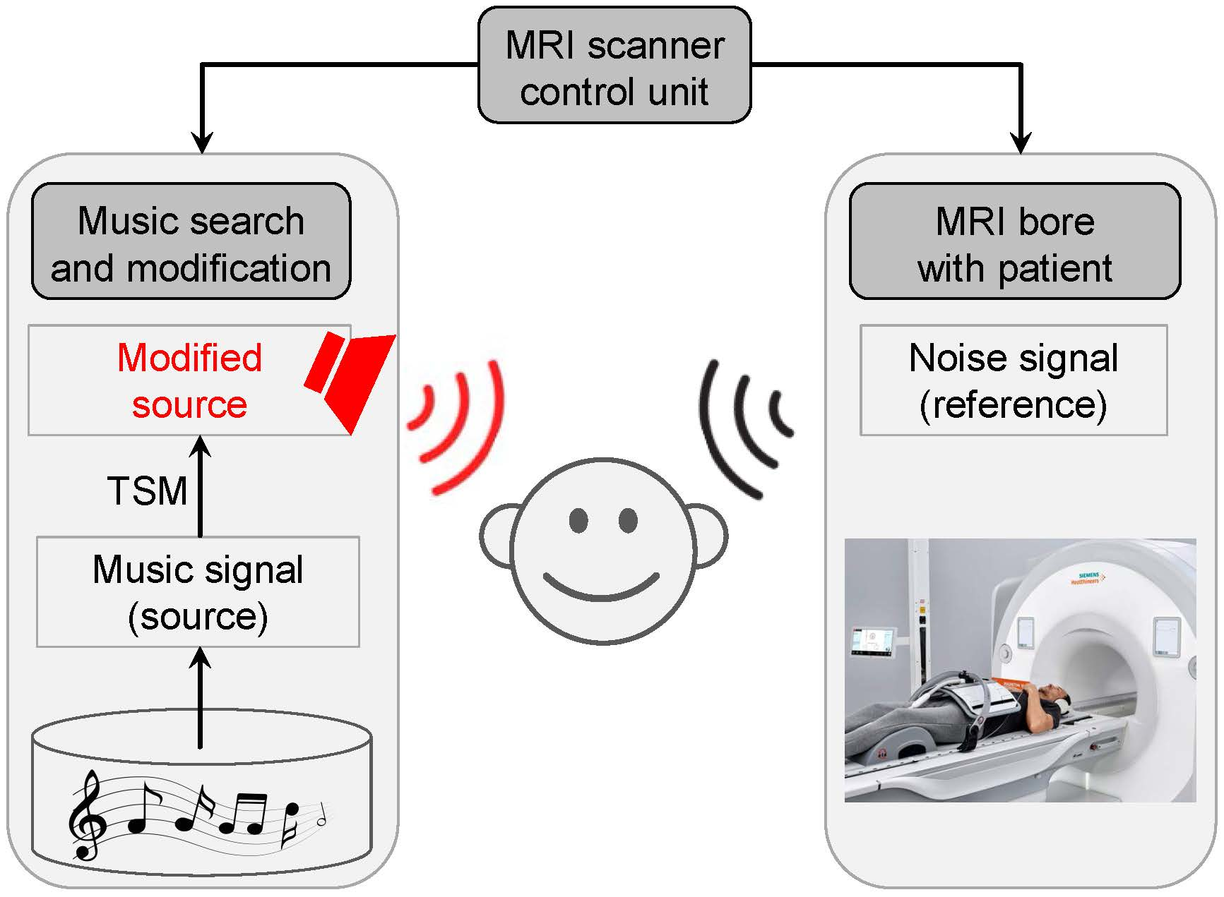
It is a generally accepted fact that ambient music may have a positive effect by inducing positive emotions, while reducing stress during certain situations [5,6]. In this paper, we consider the problem of adapting suitable music recordings to reduce the negative effects that MRI noise signals impose on patients—a process that may loosely be referred to as noise beautification [7]. In general, the acoustic aspects that may be considered in noise beautification are manifold including frequency, timbre, loudness, and time. The music may then be chosen accordingly and adapted with regard to pitch, harmony, instrumentation, volume, tempo, and beat. In the following, motivated by the characteristics of specific MRI devices, we concentrate on the aspects of time and beat. Many MRI scanners produce loud knocking sounds, which are typically spaced in a locally periodic fashion. These regular beat-like noise patterns may be interrupted by longer periods of silence. The sudden restart of the knocking sounds after these periods may introduce another source of the patient’s discomfort. Our approach for noise beautification relies on the assumption that, in contrast to loud hammering acoustic noise, rhythmically played musical sounds may act in a relaxing manner to a human listeners. By adapting the tempo of a music recording, the goal is to temporally synchronize the beat positions of the music with the regular hammering noise. In the ideal case, the noise signal becomes part of the played music, thus creating a more pleasant and less stressful acoustic environment. Furthermore, filling in the periods of silence between knocking pulse trains with music may have an additional protective effect on the listener (see also Section 2).

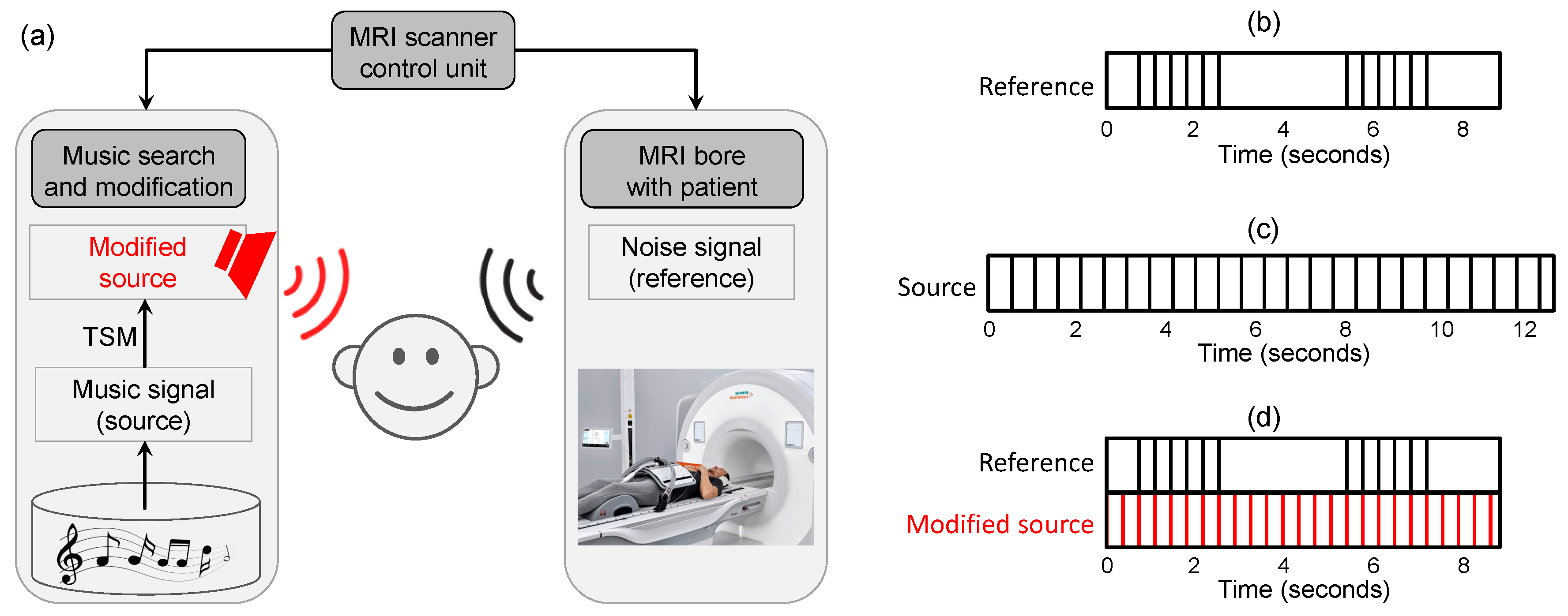
The main technical contributions of this papers are as follows. First, we formalize the problem of temporally aligning two sound signals with respect to certain constraints. The constraints are given by a reference time axis with specified time points, e.g., given by the time positions of the MRI scanner’s knocking sounds (see Figure 1b). Furthermore, a music recording yields a source time axis with specified time points that correspond to the musical beat positions. Then the goal is to temporally modify the music signal such that all reference points are superimposed by musical beats. We model this alignment task as an optimization problem, where the objective is to compute a mapping that fulfills the constraints while minimizing strong local distortions in the adapted music signals (Section 3). The latter condition, which can be expressed in terms of suitably defined second-order differences, tries to avoid strong local, unrhythmical tempo changes in the music. As a further contribution, we introduce a novel algorithm based on dynamic programming for finding an optimal solution as well as a greedy algorithm for finding an approximate solution of this optimization problem (Section 4). Based on such a mapping between reference and source time points, we then describe how to apply time-scale modification (TSM) to temporally adapt the music signal in a local fashion (Section 5). As a result, the beats of the modified music signal are in sync within the MRI scanner’s knocking sounds (see Figure 1d). Finally, we discuss the benefits and limitations of our approach to noise beautification within the MRI application scenario by presenting a number of representative real-world and synthetic examples (Section 6). Further background information and a discussion of relevant work can be found in Section 2.

2. Background

In this section, we give an overview on existing approaches that are related to our MRI-based noise beautification scenario and give pointers to relevant literature. Further related work is also discussed in the subsequent sections.

Methods to reduce the acoustic noise reaching the patient ears in an MRI environment are largely divided into passive methods and active methods. Passive methods reduce the noise by acoustic noise barriers to prevent vibration of the MRI equipment itself or by protecting the patient using ear muffs or ear plugs. However, the noise reduction performance achieved by passive methods is rather poor; it is good enough for reducing the sound pressure below a safety level that guarantees a required protection of the auditory system, but it is insufficient to avoid the patient’s discomfort during MRI. Active methods usually complement passive methods by further attenuating the acoustic noise through counteracting acoustic pressure waves. Most of these methods use an external speaker (positioned far away from the MRI magnet) and a plastic tube, which transmits the counteracting sound waves from the speaker to the patient’s ears. However, due to long acoustic paths, this solution is subject to sound field disturbances and signal delays. As a result, particularly high-frequency noise components (above 1 kHz) cannot be canceled effectively, thereby not providing satisfactory noise reduction.

In the past, various alternative methods have been suggested that neither eliminate nor attenuate the MRI acoustic noise. Instead, these methods try to circumvent the problem by trying to better “accommodate” the patient by inducing a subjectively pleasant noise perception. For example, as suggested in [2], it is possible to make use of the sound generation proprieties of the MRI gradient coils to generate additional harmonic, music-like passages at the end of each iteration of an MRI sequence during the scanning process. This idea is to break the monotony of the MRI acoustic noise by adding a succession of harmonic chords that combine into a melody, thus providing a more relaxing and calming acoustic ambient for the patients. However, this method increases the scan time as well as interferes with the evolution of nuclear spins, which may impair the image quality. Furthermore, it also does not guarantee an effective protection of the hearing organs against loud MRI noise peaks. Recognizing this problem, Schreiber [3] suggests using a power audio amplifier and loudspeakers to generate so-called protective sounds, which rise slowly in amplitude, thus increasing the impedance in the middle ear directly before the onsets of the loud MRI sounds. This invention makes use of the middle ear reflex—a mechanism the hearing of vertebrates possesses, where at high sound pressure the impedance of the auditory is adjusted to attenuate the vibration amplitudes of the small bones and tympanic membrane in the middle ear. Even though the patent [3] mentions that music may be used as a protective sound, it does not disclose a method to avoid an erratic and thereby unpleasant mixing of music and the regular noise emerging out of an MRI scanner.

In [4], Schmale and Koehler propose a method to select a suitable music piece that rhythmically matches the periodic MRI noise. The goal is to rhythmically and harmonically synchronize the complementary music piece to a specific MRI gradient sequence. Thereby, this invention coined the term of noise beautification. However, this patent does not show how an appropriate music piece for each of the many possible clinical MRI sequences (having different repetition periods) can be found—not to speak of different musical tastes of the patients. To deal with this problem, Popescu [7] suggests to use a virtual music composer, which uses audio processing techniques to determine a song’s melody, beat, tempo, rhythm, pitches, chords, sonic brilliance, timbre, and several other descriptors. Based on a multidimensional model of the song and of the expected MRI noise, the software synthesizes a new version of the song to match the noise. The goal is to rhythmically and harmonically mask the MRI acoustic noise, thus protecting the hearing organs by leveraging the middle ear reflex. Additionally, a patient’s specific musical preferences (such as genre, style, or language) as well as other data relevant to the patient’s age, ethnicity, and nationality can be taken into consideration.

Similar to the synthesis approach described in [7], our approach modifies a music recording to satisfies constraints that are imposed by the MRI scanner’s acoustic noise. In our MRI application scenario, we assume that the MRI scanner’s knocking sound patterns are known beforehand. This is a realistic assumption since there is typically a limited number of different MRI scanner settings, which are left fixed during a recording session (see [4]). In many recording situations, each such setting yields a well-defined and predictable sequence of knocking sounds (including the knowledge about the periods of silence). Therefore, one can perform the music adaptation of each of the possible settings in an offline fashion. In the actual noise beautification application, one then only needs to derive a global offset to sync the noise signal with the (precomputed) modified music signal chosen according to the respective MRI setting.

The general task of aligning and synchronizing two sound signals is not novel and plays an important role in a wide range of scenarios. For example, music producers or DJs adapt the time-scale of different music recordings in a beat-synchronous fashion for music remixing purposes for creating smooth transitions from one song to another song [8,9,10]. Another conceptually related application is proposed in [11,12], where the goal is to adapt the tempo of the music signal according to an external reference signal such as the steps of a walker or runner. Also in the production of sound tracks for movies, video games, commercials, or audio books, automated tools for adapting existing music recordings to fulfill certain temporal constraints have been studied (see, e.g., [13,14,15,16,17]). The pointers to the literature are not meant to be comprehensive and only yield some example scenarios. In all these applications, the common goal is to align specific time positions of two different time series under certain constraints. We hope that the specific alignment problem considered in this paper, the mathematical modeling, and the algorithms proposed are applicable and inspirational for other scenarios beyond our motivating MRI scenario.

3. Constraint-Based Alignment Task as Optimization Problem

In this section, we formalize our constraint-based alignment task. Recall that we are given two signals: the MRI noise signal to be superimposed and the music signal to be adapted. In this context, the noise signal serves as reference that defines the constraints, whereas the music signal serves as source that is to be modified according to the constraints. In the following, the time axis of the noise signal is referred to as reference time axis, while the time axis of the music signal is called the source time axis. In both cases, we are given a finite set of specified time points, which we also call alignment points (APs). In the case of the reference time axis, let $M\in \mathbb{N}$ be the number of APs and

$$\mathcal{R}:=\{r_1,r_2,\dots ,r_M\}$$

(1)

be the set of APs with $r_1<r_2<\dots <r_M$. Each $r_m\in \mathbb{R}$ is given in seconds, $m\in [1:M]:=\{1,2,\dots ,M\}$. Similarly, in the case of the source time axis, let $N\in \mathbb{N}$ be the number of APs and

$$\mathcal{S}:=\{s_1,s_2,\dots ,s_N\}$$

(2)

be the set of APs with $s_1<s_2<\dots <s_N$.

Based on these notions, our overall goal is to temporally modify the source signal such that the reference APs are superimposed by suitable source APs. To model an alignment between reference and source APs, we introduce a mapping function

$$\phi :\mathcal{R}\to \mathcal{S}$$

(3)

which assigns a source AP $\phi (r_m)\in \mathcal{S}$ to each of the reference APs $r_m\in \mathcal{R}$, $m\in [1:M]$. Furthermore, when modifying the source signal, we only want to apply local time-scale modifications where the temporal order of time events is preserved. Therefore, we require a monotonicity condition expressed by

$$\phi (r_m)<\phi (r_{m+1})$$

(4)

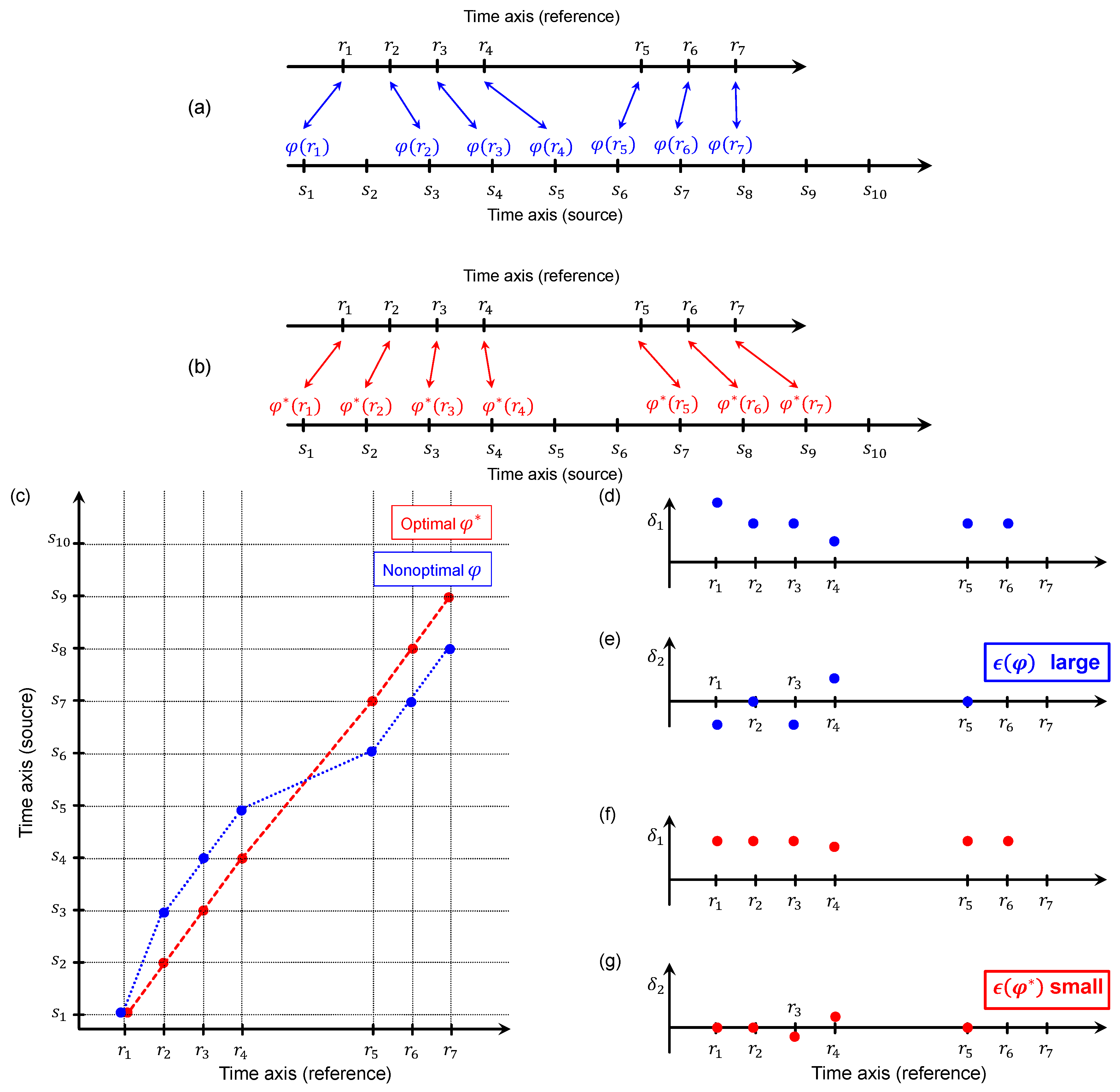
for $m\in [1:M-1]$. In the following we say that a mapping function is valid if it fulfills the monotonicity condition of Equation (4). As indicated by Figure 2, there are many possible valid mapping functions. More precisely, the number of valid mapping functions is $($. This leads to the questions which of these mapping functions are “suitable” and how to find them.

In our application scenario, we want to temporally modify the source signal by applying non-linear TSM. In the case of a music signal with a more or less steady beat, a global change in tempo may be acceptable. However, strong local changes in the tempo may result in an unrhythmical, thus unpleasant version. Motivated by this observation, we are looking for mapping functions with as little as possible local fluctuations. Intuitively, we model this requirement by introducing an error measure that depends on second-order derivatives. Based on the discrete nature of our mapping problem, we define an error function $ϵ(\phi )$ for a given valid mapping function $\phi$ as follows:

$$\begin{array}{ccc}\hfill {\delta }_1(r_m)& :=& \frac{\phi (r_{m+1})-\phi (r_m)}{r_{m+1}-r_m}\mathrm{for}m\in [1:M-1],\hfill \end{array}$$

(5)

$$\begin{array}{ccc}\hfill {\delta }_2(r_m)& :=& \frac{{\delta }_1(r_{m+1})-{\delta }_1(r_m)}{r_{m+1}-r_m}\mathrm{for}m\in [1:M-2],\hfill \end{array}$$

(6)

$$\begin{array}{ccc}\hfill ϵ(\phi )& :=& \sum _{m=1}^{M-2}\left|{\delta }_2(r_m)\right|.\hfill \end{array}$$

(7)

Obviously, there are many more ways to define suitable error measures, e.g., using the sum over squared ${\delta }_2$-values or the maximum over all ${\delta }_2$-values. The definition in Equation (7) should be regarded as one possible choice; the subsequent considerations can be applied to other error measures as well. Figure 2 illustrates the definition of our error measure by means of two examples. Based on the error measure, an optimal mapping function is defined to be

$${\phi }^{*}:=argmin\left\{ϵ(\phi )\mid \phi \mathrm{is}\mathrm{a}\mathrm{valid}\mathrm{mapping}\mathrm{function}\right\}.$$

(8)

Note that, in general, there may be more than one optimal valid mapping function.

4. Algorithms

As said before, the number of valid mapping functions $\phi$ is $($. This number explodes for increasing N and M. For example, for $N=50$ and $M=25$, one obtains $(\genfrac{}{}{0pt}{}{50}{25})\approx 1.3\times {10}^{14}$ possible functions. Therefore, a brute force algorithm to derive ${\phi }^{*}$ by simply trying out all valid mapping functions is generally computationally infeasible. In this section, we introduce a more efficient algorithm based on dynamic programming that computes ${\phi }^{*}$ in polynomial time requiring $O(N^{3}M)$ operations (Section 4.1). Since this algorithm is still too slow for large N, we describe an efficient greedy algorithm that only requires $O(N)$ operations (Section 4.2). However, this algorithm does generally not output an optimal mapping function, but only a coarse approximate solution. This approximation, as also shown in our experiments, may still be useful under specific assumptions that are motivated by our application scenario.

4.1. DP-Based Algorithm

In our first approach, we introduce an algorithm for computing an optimal mapping function using dynamic programming (DP)—an algorithmic paradigm that breaks down a problem into simpler subproblems in a recursive manner [18]. Let $\phi$ be a valid mapping function. Recall from Equation (7) that, for computing the error measure $ϵ(\phi )$, we need second-order differences ${\delta }_2(r_m)$ based on the triples $(r_m,r_{m+1},r_{m+2})\in {\mathcal{R}}^3$ and $(\phi (r_m),\phi (r_{m+1}),\phi (r_{m+2}))\in {\mathcal{S}}^3$, $m\in [1:M-2]$. In our optimization procedure, we consider all possible source triples that may occur in combination with a reference triple. In the following, we specify a source triple by a 3-element ordered subset of $\mathcal{S}$ with strictly increasing elements:

$$\gamma =(\gamma (1),\gamma (2),\gamma (3))\in {\mathcal{S}}^3\mathrm{with}\gamma (1)<\gamma (2)<\gamma (3).$$

(9)

Let $L=(\genfrac{}{}{0pt}{}{N}{3})$ be the number and $({\gamma }_1,{\gamma }_2,\dots ,{\gamma }_L)$ the list of all such source triples, where the triples are sorted in lexicographically increasing order, i.e., starting with ${\gamma }_1=(s_1,s_2,s_3)$ and ending with ${\gamma }_L=(s_{N-2},s_{N-1},s_N)$. We say that a family consisting of $M-2$ source triples specified by a list

$$({\ell }_1,{\ell }_2,\dots ,{\ell }_{M-2})\mathrm{with}1\le {\ell }_1<{\ell }_2<\dots <{\ell }_{M-2}\le L$$

(10)

is valid if two subsequent source triples overlap in two points:

$${\gamma }_{{\ell }_m}(2)={\gamma }_{{\ell }_{m+1}}(1)\mathrm{and}{\gamma }_{{\ell }_m}(3)={\gamma }_{{\ell }_{m+1}}(2)\mathrm{for}m\in [1:M-3].$$

(11)

Such a valid family obviously defines a valid mapping function $\phi$ by setting:

$$\phi (r_m)=\left\{\begin{array}{cc}{s}_n\mathrm{with}n={\gamma }_{{\ell }_m}(1),\hfill & \mathrm{for}m\in [1:M-2],\hfill \\ s_n\mathrm{with}n={\gamma }_{{\ell }_{M-2}}(2),\hfill & \mathrm{for}m=M-1,\hfill \\ s_n\mathrm{with}n={\gamma }_{{\ell }_{M-2}}(3),\hfill & \mathrm{for}m=M.\hfill \end{array}\right.$$

(12)

Vice versa, each valid mapping function $\phi$ yields a valid family of source triples given by $(\phi (r_m),\phi (r_{m+1}),\phi (r_{m+2}))\in {\mathcal{S}}^3$ for $m\in [1:M-2]$. In other words, there is a one-to-one correspondence between valid mapping functions and valid families of source triples having size $M-2$.

Given a reference triple $(r_m,r_{m+1},r_{m+2})$ for $m\in [1:M-2]$ and a source triple ${\gamma }_{\ell }$ for $\ell \in [1:L]$, we define, similar to Equation (6), the second-order difference

$${\delta }_2(\ell ,m):=\frac{1}{r_{m+1}-r_m}\left(\frac{{\gamma }_{\ell }(3)-{\gamma }_{\ell }(2)}{r_{m+2}-r_{m+1}}-\frac{{\gamma }_{\ell }(2)-{\gamma }_{\ell }(1)}{r_{m+1}-r_m}\right).$$

(13)

Furthermore, we define

$$ϵ(({\ell }_1,{\ell }_2,\dots ,{\ell }_m)):=\sum _{k=1}^m\left|{\delta }_2({\ell }_k,k)\right|$$

(14)

for any valid family, specified by $({\ell }_1,{\ell }_2,\dots ,{\ell }_m)$, of size $m\in [M-2]$. Obviously, for a family of size $m=M-2$, this definition leads to the same error measure as defined in Equation (7).

With these definitions at hand, we now describe our DP-based algorithm for computing an optimal valid mapping function or, equivalently, an optimal family of source triples of size $M-2$. To this end, we consider the following subproblem for each $m\in [M-2]$ and $\ell \in [1:L]$:

$$\mathbf{D}(\ell ,m):=min\left\{ϵ(({\ell }_1,{\ell }_2,\dots ,{\ell }_m))\mid ({\ell }_1,{\ell }_2,\dots ,{\ell }_m)\mathrm{is}\mathrm{valid}\mathrm{and}{\ell }_m=\ell \right\}.$$

(15)

In other words, $\mathbf{D}(\ell ,m)$ yields the minimal error for mapping the first m reference APs $r_1,r_2,\dots ,r_m$ to source APs using a valid mapping function with the additional constraint that the last triple is given by ${\gamma }_{\ell }$. In the case that such a mapping function does not exist (i.e., that the set in Equation (15) is empty), we set $\mathbf{D}(\ell ,m):=\infty$. The matrix $\mathbf{D}\in {\mathbb{R}}^{L\times (M-2)}$ can be computed recursively in a columnwise fashion. For $m=1$, one has

$$\mathbf{D}(\ell ,1)=|{\delta }_2(\ell ,1)|.$$

(16)

Furthermore, for $m=2,\dots ,M-2$ one can compute $\mathbf{D}(\ell ,m)$ as follows:

$$\mathbf{D}(\ell ,m)=|{\delta }_2(\ell ,m)|+min\left\{\mathbf{D}(k,m-1)\mid k\in [1:L]\mathrm{with}{\gamma }_k(2)={\gamma }_{\ell }(1)\mathrm{and}{\gamma }_k(3)={\gamma }_{\ell }(2)\right\},$$

(17)

where the minimum over an empty set is again defined to be infinite.

From the matrix $\mathbf{D}$ one can obtain the minimal error of a valid source triple family of size $M-2$ or, equivalently, the minimal error of an optimal valid mapping function ${\phi }^{*}$, by looking at the minimal value of the last column (specified by $m=M-2$) of $\mathbf{D}$:

$$ϵ({\phi }^{*})=min\left\{\mathbf{D}(\ell ,M-2)\mid \ell \in [1:L]\right\}.$$

(18)

Starting with the triple ${\gamma }_{{\ell }_{M-2}}$ defined by

$${\ell }_{M-2}:=argmin\left\{\mathbf{D}(\ell ,M-2)\mid \ell \in [1:L]\right\},$$

(19)

one can iteratively obtain ${\gamma }_{{\ell }_{M-3}},\dots ,{\gamma }_{{\ell }_1}$ by backtracking the minimizing indices in Equation (15) for $m=M-3,M-4,\dots ,1$. Since this backtracking step is a standard approach in DP, we do not discuss here in this paper, but refer to the literature (e.g., [18]) for details.

Using suitable data structures in the minimization of Equation (17), the overall algorithmic complexity of our algorithm is determined by the size of the matrix $\mathbf{D}$, which is $O(LM)=O(N^{3}M)$. For $N=50$ and $M=25$, for example, the number of operations is in the order of ${50}^3\times 25\approx 3\times {10}^6$, compared to $(\genfrac{}{}{0pt}{}{50}{25})\approx 1.3\times {10}^{14}$ using a brute force algorithm. Still, for large N and M, this algorithm may be too slow for real-world applications. One possible strategy is to apply a multi-stage approach, where, in the first stage, a coarse mapping is computed efficiently, e.g., using a greedy strategy based on suitable heuristics. This coarse mapping can then be further “refined” by applying the DP-based approach only locally. Similar approaches have been successfully used for time alignment approaches based on dynamic time warping (see, e.g., [19], Chapter 4).

4.2. Greedy Algorithm

We now introduce an efficient greedy algorithm for finding an approximate solution for our mapping problem. This algorithm makes strong assumptions (motivated by our MRI noise beautification scenario) on how the reference and source APs are distributed over time. In our application, the reference APs $\mathcal{R}=\{r_1,r_2,\dots ,r_M\}$ (corresponding to the MRI scanner’s knocking sounds) are typically spaced in a locally periodic fashion for most of the time. Similarly, the same holds for the source APs $\mathcal{S}=\{s_1,s_2,\dots ,s_N\}$ (corresponding to the beats of the music). In other words, there are positive numbers ${\Delta }^{\mathcal{R}},{\Delta }^{\mathcal{S}}\in \mathbb{R}$ such that

$$r_{m+1}-r_m\approx {\Delta }^{\mathcal{R}}\mathrm{and}{s}_{n+1}-s_n\approx {\Delta }^{\mathcal{S}}$$

(20)

for most of the $m\in [1:M-1]$ and $n\in [1:N-1]$, respectively. Based on this assumption, we define a global scaling factor

$$\sigma :=\frac{{\Delta }^{\mathcal{R}}}{{\Delta }^{\mathcal{S}}}.$$

(21)

Furthermore, we assume that the mapping for the first reference AP $r_1$ is known and equals $s_{n_1}\in \mathcal{S}$ for some $n_1\in [1:N]$. The scaling factor $\sigma$ and source AP $s_{n_1}$ are used to globally normalize and rescale the source APs:

$${\tilde{s}}_n:=\sigma ·(s_n-s_{n_1})+r_1.$$

(22)

for $n\in [1:N]$. Defining $\phi (r_1):=s_{n_1}$, we step through the reference APs and iteratively define $\phi (r_m)$ for $m=2,3,\dots ,M$. Assuming that $\phi (r_{m-1})=s_{n_{m-1}}$ for some $n_{m-1}\in [1:N]$, we define $\phi (r_m):=s_{n_m}$ with

$$n_m:=argmin\left\{|r_m-{\tilde{s}}_n|\mid n\in [n_{m-1}+1:N]\right\}.$$

(23)

Note that the condition $n_m>n_{m-1}$ ensures the monotonicity condition of $\phi$. Furthermore, note that the greedy algorithm only yields a mapping function if $n_m<N$ for all $m\in [1:M-1]$. This is typically the case when the number N of source APs is much larger then the number M of reference APs.

Intuitively speaking, using the globally scaled version of source APs (as defined in Equation (21)) compensates for “tempo differences” between the reference MRI signal and the source music signal. Furthermore, the minimization in Equation (23) compensates for small local deviations between reference and source APs. In regions of periodically spaced reference APs (with period ${\Delta }^{\mathcal{R}}$) and source APs (with period ${\Delta }^{\mathcal{S}}$), the second-order differences in the resulting mapping is close to zero for most of the time, thus resulting in a low error. Also, this holds if differences between subsequent APs are integer multiples of ${\Delta }^{\mathcal{R}}$ and ${\Delta }^{\mathcal{S}}$, respectively. Only if there are many local irregularities in the reference or the source, the resulting mapping may yield a poor approximation of the optimal solution. Finally, note that the proposed greedy strategy may be locally refined by the DP-based approach as discussed at the end of Section 4.1.

5. Adaption Using Time-Scale Modification (TSM)

We now describe how we apply time-scale modification (TSM) to adapt the source signal to run synchronously along the reference signal. As described in the introduction, TSM is a procedure for modifying the duration of a given audio signal while preserving other properties such as pitch and timbre. In a typical TSM approach, the input signal is decomposed into short frames of a fixed length, typically in the range of 50 to 100 milliseconds. The frames are then relocated on the time axis to achieve the actual time-scale modification, while, at the same time, preserving the signal’s pitch (see [20] for an overview).

Many TSM algorithms allow for stretching or compressing the signal by a constant factor. In our scenario, however, the time axis needs to be modified in a non-linear fashion. Such a non-linear modification can be formally described by a time-stretch function, which is a strictly monotonously increasing function $\tau :\mathbb{R}\to \mathbb{R}$ yielding a continuous mapping between input time points (given in seconds) and output time points. Based on such a continuous time-stretch function $\tau$, as described in [20], one can convert basically all frame-based global TSM procedures into non-linear versions. The main idea of the conversion is to fix an equidistant time grid for synthesis frame positions that will be used to generate the output signal. Then, for every grid point, the inverse of $\tau$ is used to identify an analysis frame position of the input signal. Finally, these non-linearly spaced analysis frames are used as linearly spaced synthesis frames to construct a modified signal that has the desired local tempo changes. For details, we refer to [20].

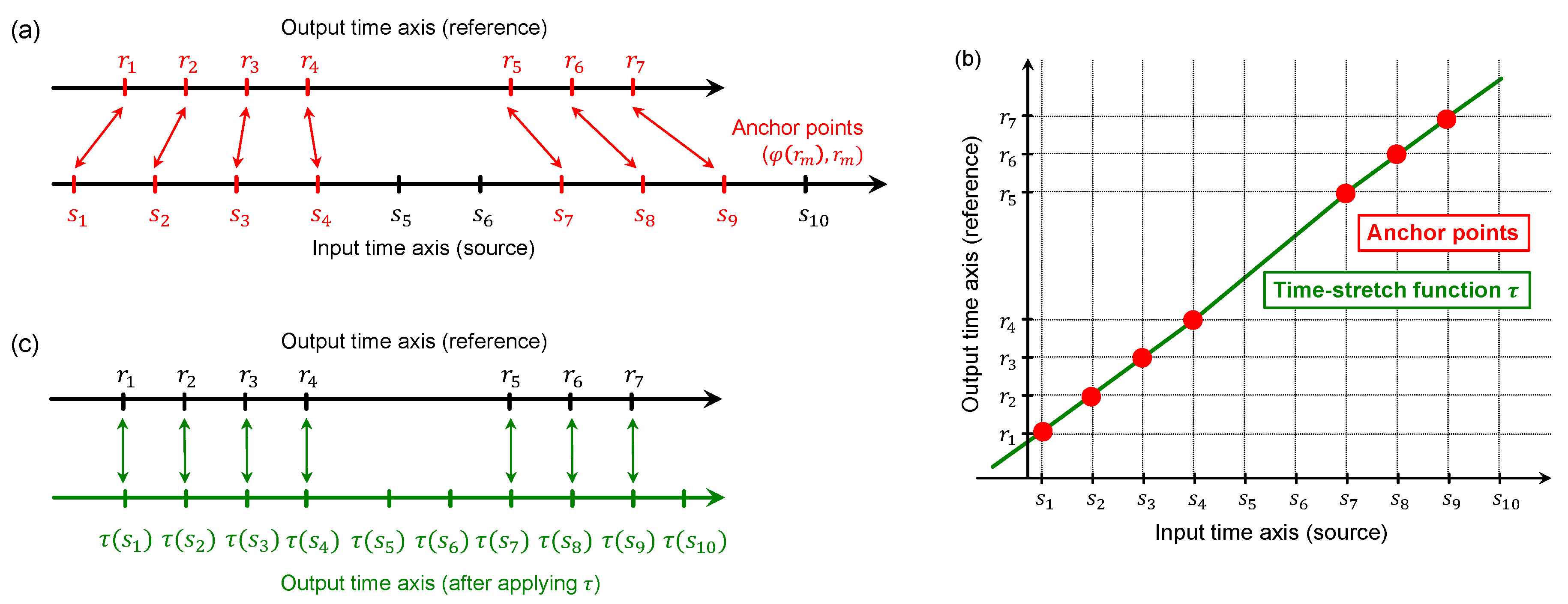
In our scenario, the source signal serves as input signal that needs to be modified. Recall that a valid mapping function $\phi$ defines a mapping between reference APs $r_m$ and source APs $\phi (r_m)$, $m\in [1:M]$. We use this mapping to define the pairs $(\phi (r_m),r_m)\in \mathcal{S}\times \mathcal{R}$, which we call anchor points (see Figure 3a). Based on these anchor points, we define a time-stretch function $\tau$ within the intervall $[\phi (r_1),\phi (r_M)]$ by applying linear interpolation between these anchor points (see Figure 3b). Finally, one can extend $\tau$ to the left of $\phi (r_1)$ and to the right of $\phi (r_M)$ in a linear fashion with a slop as defined for the subsequent and previous interval, respectively. Based on this time-stretch function $\tau$, one can then apply a non-linear TSM procedure as described in the previous paragraph to modify the source signal. In the resulting time axis of the output signal, the mapped source APs are now in sync with the reference APs (see Figure 3c).

As summarized in [20], there are different types of frame-based TSM procedures including the waveform similarity overlap-add (WSOLA) approach [21] or the phase vocoder (PV) approach [22,23,24]. Some of the procedures are designed to preserve the perceptual quality of harmonic signal components, while introducing undesired artifacts in the presence of sudden transient-like signal components. Other TSM procedures can better preserve the sharpness of percussive elements, while having problems in preserving the characteristics of harmonic passages. To reduce unwanted artifacts on both sides, we use the combined TSM procedure introduced in [25]. The idea is to first separate the input signal into a harmonic and a percussive component, then to process each component with a different TSM procedure that preserves its respective characteristics, and finally to generate the output signal by superimposing the processed harmonic and percussive component. For our experiments, we used a publicly available MATLAB implementation of this combined TSM procedure contained in the TSM toolbox [26] (https://www.audiolabs-erlangen.de/resources/MIR/TSMtoolbox).

6. Experiments

To illustrate the outcome of our noise beautification approach, we now report on experiments based on reference and source signals of various types and complexity. To make the results audible and comprehensible for the reader, the original signals as well as the experimental results have been made publicly available on the website: https://www.audiolabs-erlangen.de/resources/MIR/2018-MRI-NoiseBeauty, under a suitable Creative Commons license. The reference signals include recordings of four representative MRI noise signals, everyday noise, as well as synthetically generated pulse click tracks. An overview of these reference signals along with a short description and identifiers can be found in

Table 1. Reference (noise) signals used in our experiments.

ID	Type	Description	Tempo (BPM)	Length (s)
$\mathtt{R}-\mathtt{MRI}-\mathtt{06}$	MRI	Locally periodic pulse sound interrupted by longer gaps, with additional tick sounds	267	18.1
$\mathtt{R}-\mathtt{MRI}-\mathtt{12}$	MRI	Periodic pulse sound	250	18.1
$\mathtt{R}-\mathtt{MRI}-\mathtt{20}$	MRI	Periodic knocking sound	240	17.7
$\mathtt{R}-\mathtt{MRI}-\mathtt{24}$	MRI	Locally periodic pulse sound interrupted by short gaps	367	18.0
$\mathtt{R}-\mathtt{RW}-\mathtt{Heart}$	Real world	Heartbeat sound	200	21.6
$\mathtt{R}-\mathtt{RW}-\mathtt{Snore}$	Real world	Snoring sound	16	62.1
$\mathtt{R}-\mathtt{RW}-\mathtt{Train}$	Real world	Sound of an accelerating steam train	190→285	20.0
$\mathtt{R}-\mathtt{RW}-\mathtt{Water}$	Real world	Tap dripping sound	99	18.4
$\mathtt{R}-\mathtt{Syn}-\mathtt{Co}$	Synthetic	Click track with constant tempo	150	30.0
$\mathtt{R}-\mathtt{Syn}-\mathtt{CoGa}$	Synthetic	As $\mathtt{R}-\mathtt{Syn}-\mathtt{CoGa}$ with longer gaps	150	30.0
$\mathtt{R}-\mathtt{Syn}-\mathtt{CoIrGa}$	Synthetic	As $\mathtt{R}-\mathtt{Syn}-\mathtt{CoGa}$ with local irregularities	150	30.0
$\mathtt{R}-\mathtt{Syn}-\mathtt{In}$	Synthetic	Click track with increasing tempo	78→450	18.7
$\mathtt{R}-\mathtt{Syn}-\mathtt{InGa}$	Synthetic	As $\mathtt{R}-\mathtt{Syn}-\mathtt{In}$ with longer gaps	78→450	18.7
$\mathtt{R}-\mathtt{Syn}-\mathtt{InIrGa}$	Synthetic	As $\mathtt{R}-\mathtt{Syn}-\mathtt{InIrGa}$ with local irregularities	78→429	18.7
$\mathtt{R}-\mathtt{Syn}-\mathtt{Ra}$	Synthetic	Click track with random distances	−	30.0
$\mathtt{R}-\mathtt{Syn}-\mathtt{RaGa}$	Synthetic	As $\mathtt{R}-\mathtt{Syn}-\mathtt{Ra}$ with longer gaps	−	30.0

. For example, the signal $\mathtt{R}-\mathtt{MRI}-\mathtt{06}$ is an MRI signal that consists of periodically spaced knocking sounds interleaved with periods of silence (see Figure 6a). As for the source signals, we used four music signals of different genre.

Table 2. Source (music) signals used in our experiments.

ID	Type	Description	Tempo (BPM)	Length (s)
$\mathtt{S}-\mathtt{Bach}$	Music	J. S. Bach: Prelude in C Major BWV 846 (performed by Kevin MacLeod)	200 (sixteenth)	178.7
$\mathtt{S}-\mathtt{Broke}$	Music	Broke For Free: Something Elated	176 (eighth)	234.7
$\mathtt{S}-\mathtt{Fandango}$	Music	The Freak Fandango Orchestra: Requiem for a Fish	139 (quarter)	220.7
$\mathtt{S}-\mathtt{Silence}$	Music	Silence Is Sexy: Holiday (instrumental version)	68 (quarter)	274.6

yields a description of these music recordings.

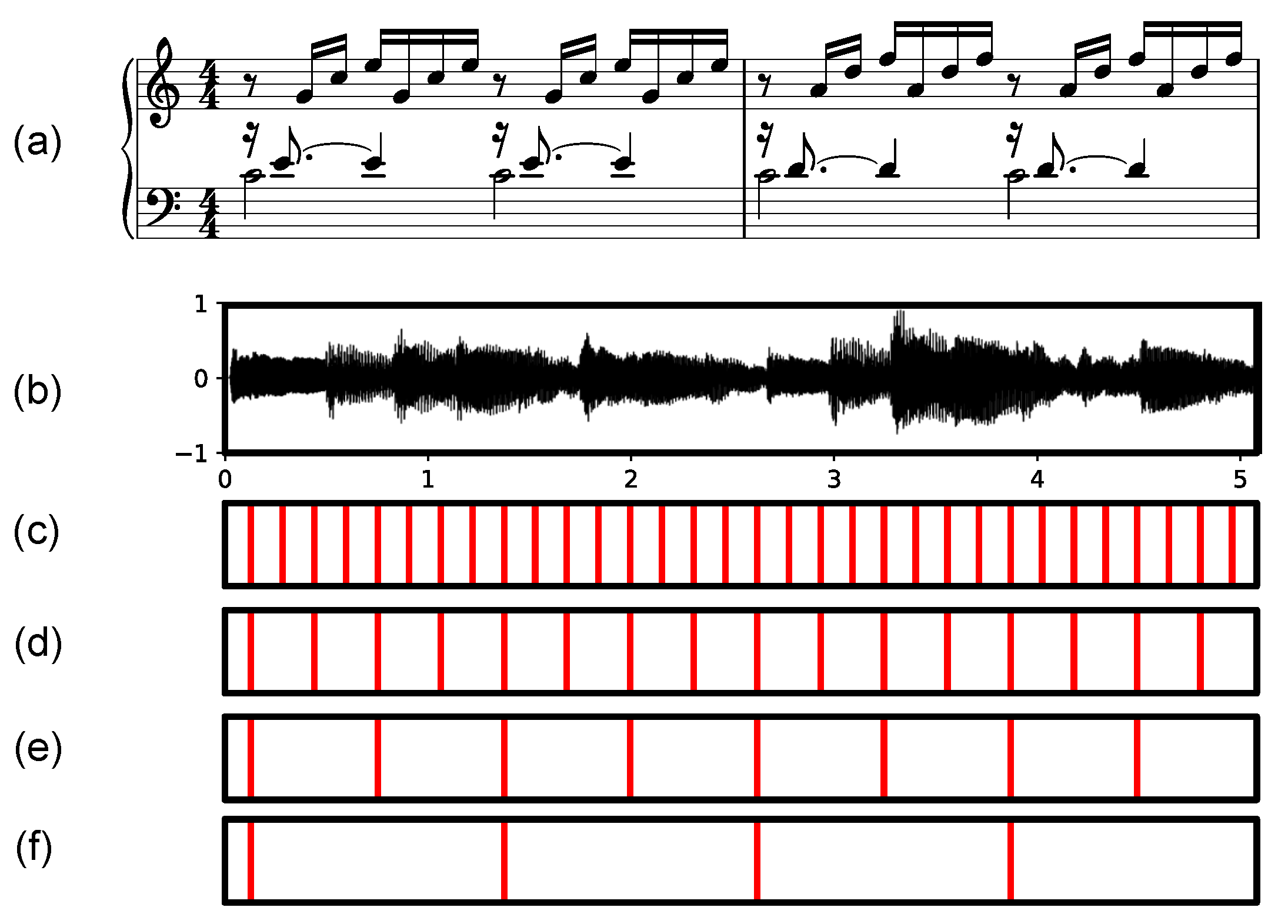
In a preprocessing step, we determined suitable APs for all reference and source signals. To this end, we applied automated onset and pulse tracking procedures as described in [27] (Chapter 6). As for the reference signals, a simple onset detector (see, e.g., [28]) was sufficient to determine the positions of the transient-like knocking or clicking noise sounds. These positions define the reference APs. As for the source signals, we first specified the rough tempo that corresponds to the metrical level (e.g., sixteenth, eighth, quarter, or half note level) to be considered. Figure 4 illustrates this by means of the source signal $\mathtt{S}-\mathtt{Bach}$. Then, we applied the predominant pulse tracking procedure from [29] to determine the positions of the pulses on that level. These positions define the source APs. In our experiments, we used implementations provided by the publicly available tempogram toolbox (https://www.audiolabs-erlangen.de/resources/MIR/tempogramtoolbox) (see [30]) as well as a beat tracker by Dan Ellis (https://labrosa.ee.columbia.edu/projects/coversongs) (see [31]).

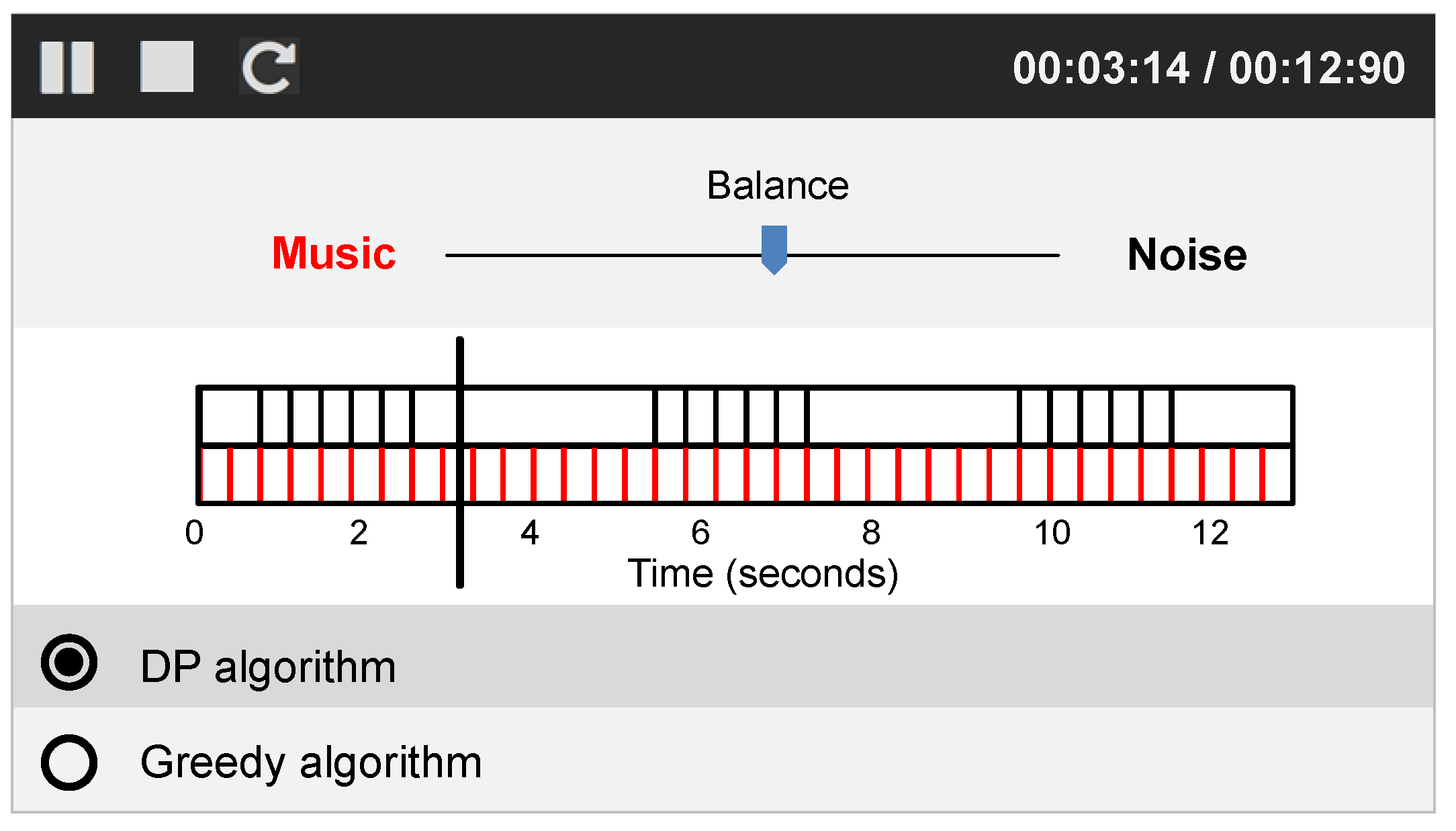
Based on the reference APs of a noise signal and the source APs of a music signal, we then applied the DP-based algorithm (see Section 4.1) as well as the greedy algorithm (see Section 4.2) to determine a mapping function. Subsequently, we utilized the procedure from Section 5 to temporally adapt the source signal to run synchronously to the reference signal. Finally, we generated an audio file, where we superimposed the original reference signal with the modified source signal. This audio file represents our final output. To evaluate the result, we also visualized the positions of the reference APs and of the modified source APs as in Figure 1d. The visualization along with the audio file was then integrated into an interactive website using the trackswitch.js framework [32] (https://audiolabs.github.io/trackswitch.js). Providing switching and playback functionalities for the audio files while synchronously indicating the playback position within the visualizations, this website allows for understanding, navigating, and evaluating the results of our noise beautification approach (see Figure 5). In particular, the balance between the reference signal and the modified source signal can be adjusted by a scroll bar. Furthermore, the output of the DP-based and greedy approach can be easily compared by the switching functionality.

On the website (https://www.audiolabs-erlangen.de/resources/MIR/2018-MRI-NoiseBeauty) mentioned above, one can find the output for all combinations consisting of a reference signal (Table 1) and a source signal (Table 2). Rather than presenting a full-fledged working system for the MRI noise beautification application, these examples indicate the behavior of our approach for different types of noise and music signals. The proof for the actual usability in a real MRI scanning session and the patients’ acceptance of such a system under the various constraints of a real medical examination is beyond the scope of this paper. However, we hope that the techniques proposed are useful for the design of such systems.

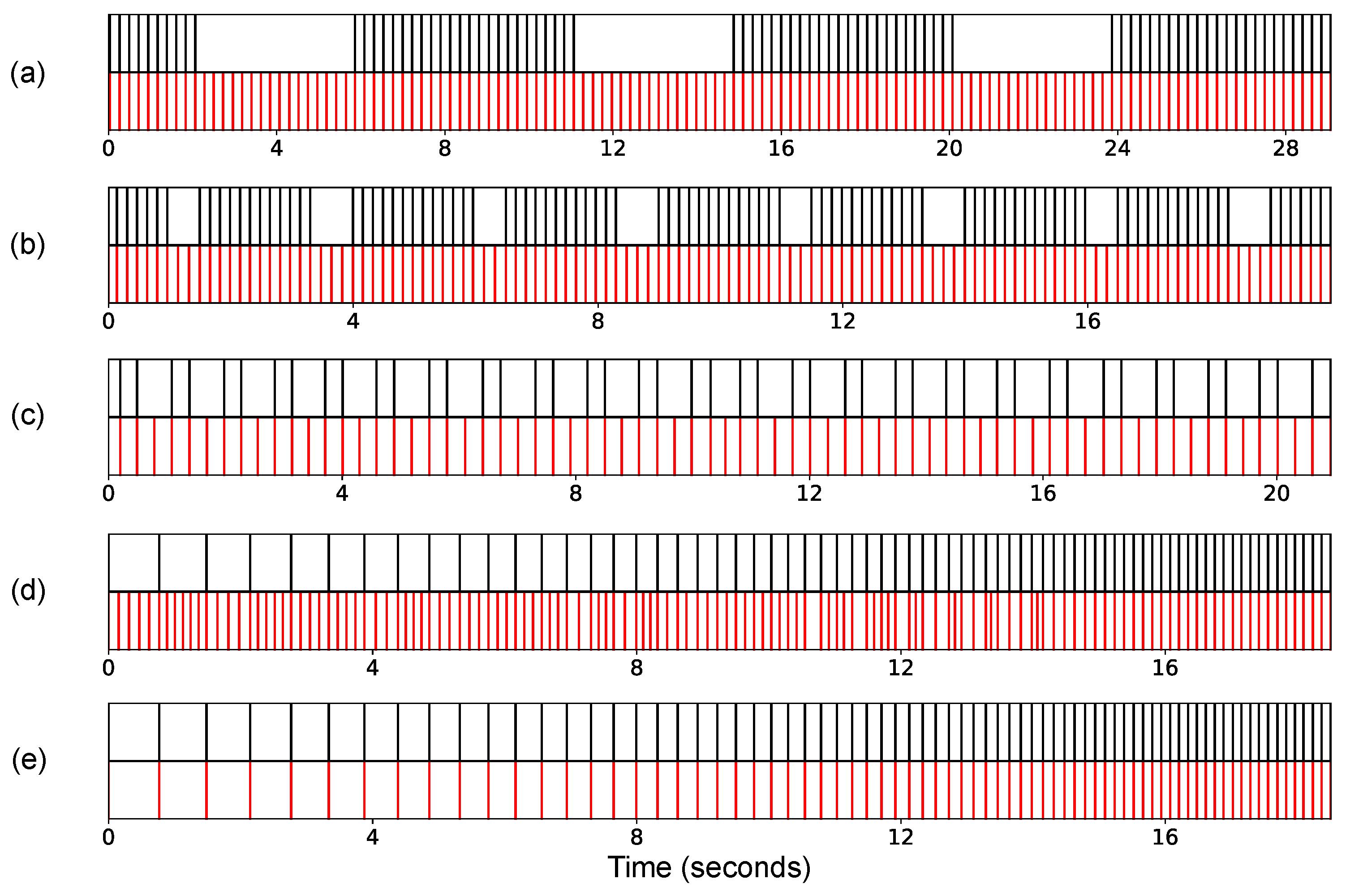
We conclude this section by having a closer look at some representative examples and report on some of our observations when conducting informal listening tests (see Figure 6). We start with the MRI noise signal R-MRI-06, which also served as a motivating example throughout the paper. This signal consists of periodically spaced knocking sounds at a rate of 4–5 beats per second (corresponding to a tempo of about 267 BPM), which are interleaved with periods of silence (see Figure 6a). In the figure, the recording $\mathtt{S}-\mathtt{Bach}$ (Prelude in C Major by J. S. Bach, see Figure 4) was used as source signal using the sixteenth-note pulse level (having a tempo of about 200 BPM at that level) to define the source APs. As shown by Figure 6a, the reference APs were matched to source APs, while the periods of silence in the reference signal R-MRI-06 were filled without introducing local temporal distortions in the modified source signal. When listening to the superposition of the noise signal and the adaptive music signal, no major artifacts can be noticed in the music.

A similar example is shown in Figure 6b. While the pulse trains of the noise signal R-MRI-24 are spaced again in a locally periodic fashion, the periods of silence between these pulse trains occur in a more irregular fashion. Still our approach is capable of mapping the eighth-note pulse grid of the music signal $\mathtt{S}-\mathtt{Fandango}$ to superimpose the knocking sounds of the MRI signal without introducing too much local distortions in the music. Besides the temporal adjustment, the selection of suitable music pieces serving as source signals is also crucial in a noise beautification scenario. In particular, the selection may be based on a patient’s personal taste or on perceptual criteria. For example, the Balkan rock music piece $\mathtt{S}-\mathtt{Fandango}$ may be more suitable to blend with the knocking sounds produced by the MRI scanner than the piano piece by Bach. When selecting a piece of music, aspects such as harmony or timbre are important cues to blend the noise and music signal [4,7]. Also, higher-level temporal structures (e.g., the meter or regularly recurring patterns such as a riff) and boundaries between musical parts may be considered as additional constraints in the mapping process. Incorporating such cues into the music selection, mapping, and adaption processes constitutes interesting research directions.

As a third illustrative example, Figure 6c shows a heartbeat signal with the typical “lub-dub, lub-dub” patterns used that define the references APs. When using our DP-based mapping approach, the sixteenth-note pulse grid of the source signal $\mathtt{S}-\mathtt{Bach}$ is nicely mapped onto these patterns, where every third pulse of the music falls into a period of silence (between a “dub” and the subsequent “lub”). This way, all the “lub-dub, lub-dub” reference APs are superimposed, while the music signal has a nearly constant tempo. Even though generally leading to similar results, local outliers occur more often for the greedy approach compared to the DP-based one. This is also illustrated when listening to the superimposed signals provided on our websites.

As a final example, we consider the synthetic noise signal $\mathtt{R}-\mathtt{Syn}-\mathtt{In}$ as reference signal, which consists of a click-track of increasing speed (starting with 78 BPM and ending with 450 BPM). Note that even though our mapping algorithms were designed to cope with locally periodic pulse tracks (as occurring in our MRI application), this non-periodic reference signal nicely illustrates the behavior of our approaches. The greedy strategy maps the source APs to the reference APs while trying to keep the overall musical pulse at a constant tempo. As a result, as illustrated by Figure 6d, the gaps (of decreasing size) between subsequent references APs are filled with a decreasing number of source APs. Using our DP-based strategy yields the solution as shown in Figure 6e. Here, the source APs are mapped to the reference APs also with increasing tempo, which minimizes the accumulated second order differences.

7. Conclusions

In this paper, we considered an application of various music processing techniques (including onset detection, pulse tracking, and time scale modification) to a concrete problem of practical relevance (MRI noise beautification). Our contribution was based on the general idea to play back suitably adjusted ambient music to decrease a patient’s discomfort when exposed to hammering acoustic noise during MRI scanning. In particular, this has led to an alignment problem with the objective to temporally modify a given music signal such that its beats are synchronized with the MRI scanner’s knocking sound. As main technical contributions, we introduced an optimization problem that formalizes this constraint-based alignment task. Furthermore, we described two algorithmic approaches, one yielding an optimal solution and the other an approximate solution for our optimization problem. Furthermore, we showed how existing TSM algorithms can be applied in a non-linear fashion to modify the music signal according to the computed alignment. Finally, we discussed some experiments based on real-world and synthetic examples to indicate the potential of our approach. Of course, to demonstrate the practicability of our approach, one needs to test such techniques in real MRI scanning scenarios with real patients. This will require sophisticated and complex studies that are far beyond the scope of this paper. Rather than presenting a full-fledged working system, our general motivation for this paper was to introduce an application scenario of practical relevance and to show how this leads to new challenging algorithmic problems. In particular, we hope that our approach is inspirational for research in noise beautification beyond the considered MRI scenario.

References

- McRobbie, D.W.; Moore, E.A.; Graves, M.J.; Prince, M.R. (Eds.) MRI from Picture to Proton; Cambridge University Press: Cambridge, UK, 2003. [Google Scholar]
- Nitz, W. Method for Operating a Magnetic Resonance Device Using a Gradient Pulse Sequence So That Two Impulses Combine to Form an Acoustic Harmonic So That Mechanical Noise Caused by the Gradient Pulses Is Reduced. DE 10043476A1/200. 2000. Available online: https://register.dpma.de/DPMAregister/pat/PatSchrifteneinsicht?docId=DE10043476A1 (accessed on 12 March 2018).
- Schreiber, A. Device for Protecting the Hearing From Loud MRT Sounds. DE10043476A1/2005. 2005. Available online: https://register.dpma.de/DPMAregister/pat/PatSchrifteneinsicht?docId=DE102005000848B3 (accessed on 12 March 2018).
- Schmale, I.; Koehler, T. Gradient Coil Noise Masking for Mpi Device. EP2313794A1. 2008. Available online: https://patentscope.wipo.int/search/en/detail.jsf?docId=WO2010018534 (accessed on 12 March 2018).
- Tsivian, M.; Qi, P.; Kimura, M.; Chen, V.H.; Chen, S.H.; Gan, T.J.; Polascik, T.J. The effect of noise-cancelling headphones or music on pain perception and anxiety in men undergoing transrectal prostate biopsy. Urology 2012, 79, 32–36. [Google Scholar] [CrossRef] [PubMed]
- Ko, C.H.; Chen, Y.Y.; Wu, K.T.; Wang, S.C.; Yang, J.F.; Lin, Y.Y.; Lin, C.I.; Kuo, H.J.; Dai, C.Y.; Hsieh, M.H. Effect of music on level of anxiety in patients undergoing colonoscopy without sedation. J. Chin. Med. Assoc. 2017, 80, 154–160. [Google Scholar] [CrossRef] [PubMed]
- Popescu, S. MR synchronous music. J. Tech. Up2date #06 2013. [Google Scholar] [CrossRef]
- Cliff, D. Hang the DJ: Automatic Sequencing and Seamless Mixing of Dance-Music Tracks; Technical Report; HP Laboratories: Bristol, UK, 2000. [Google Scholar]
- Ishizaki, H.; Hoashi, K.; Takishima, Y. Full-automatic DJ mixing system with Optimal tempo adjustment based on measurement function of user discomfort. In Proceedings of the International Society for Music Information Retrieval Conference (ISMIR), Kobe, Japan, 26–30 October 2009; pp. 135–140. [Google Scholar]
- Jehan, T. Creating Music by Listening. Ph.D. Thesis, Massachusetts Institute of Technology, Cambridge, MA, USA, 2005. [Google Scholar]
- Moens, B.; van Noorden, L.; Leman, M. D-jogger: Syncing music with walking. In Proceedings of the 7th Sound and Music Computing Conference, Barcelona, Spain, 21–24 July 2010; pp. 451–456. [Google Scholar]
- Moens, B.; Muller, C.; van Noorden, L.; Franěk, M.; Celie, B.; Boone, J.; Bourgois, J.; Leman, M. Encouraging Spontaneous Synchronisation with D-Jogger, an Adaptive Music Player that Aligns Movement and Music. PLoS ONE 2014, 9, e114234. [Google Scholar] [CrossRef] [PubMed] [Green Version]
- Liu, Z.; Wang, C.; Bai, Y.; Wang, H.; Wang, J. Musiz: A Generic Framework for Music Resizing with Stretching and Cropping. In Proceedings of the 19th ACM International Conference on Multimedia, Scottsdale, AZ, USA, 28 November–1 December 2011; pp. 523–532. [Google Scholar]
- Müller, M.; Driedger, J. Data-driven sound track generation. In Multimodal Music Processing; Müller, M., Goto, M., Schedl, M., Eds.; Dagstuhl Follow-Ups; Schloss Dagstuhl–Leibniz-Zentrum für Informatik: Dagstuhl, Germany, 2012; Volume 3, pp. 175–194. [Google Scholar]
- Wenger, S.; Magnor, M. Constrained example-based audio synthesis. In Proceedings of the 2011 IEEE International Conference on Multimedia and Expo (ICME 2011), Barcelona, Spain, 11–15 July 2011. [Google Scholar]
- Wenger, S.; Magnor, M. A Genetic Algorithm for Audio Retargeting. In Proceedings of the 20th ACM International Conference on Multimedia, Nara, Japan, 29 October–2 November 2012; pp. 705–708. [Google Scholar]
- Wenner, S.; Bazin, J.C.; Sorkine-Hornung, A.; Kim, C.; Gross, M. Scalable Music: Automatic Music Retargeting and Synthesis. Comput. Graph. Forum 2013, 32, 345–354. [Google Scholar] [CrossRef]
- Cormen, T.H.; Leiserson, C.E.; Rivest, R.L.; Stein, C. Introduction to Algorithms, 3rd ed.; The MIT Press: Cambridge, MA, USA, 2009. [Google Scholar]
- Müller, M. Information Retrieval for Music and Motion; Springer: Berlin/Heidelberg, Germany, 2007. [Google Scholar]
- Driedger, J.; Müller, M. A Review on Time-Scale Modification of Music Signals. Appl. Sci. 2016, 6, 57. [Google Scholar] [CrossRef]
- Verhelst, W.; Roelands, M. An overlap-add technique based on waveform similarity (WSOLA) for high quality time-scale modification of speech. In Proceedings of the IEEE International Conference on Acoustics, Speech, and Signal Processing (ICASSP), Minneapolis, MN, USA, 27–30 April 1993. [Google Scholar]
- Flanagan, J.L.; Golden, R.M. Phase Vocoder. Bell Syst. Tech. J. 1966, 45, 1493–1509. [Google Scholar] [CrossRef]
- Portnoff, M.R. Implementation of the digital phase vocoder using the fast Fourier transform. IEEE Trans. Acoust. Speech Signal Process. 1976, 24, 243–248. [Google Scholar] [CrossRef]
- Laroche, J.; Dolson, M. Improved phase vocoder time-scale modification of audio. IEEE Trans. Speech Audio Process. 1999, 7, 323–332. [Google Scholar] [CrossRef]
- Driedger, J.; Müller, M.; Ewert, S. Improving Time-Scale Modification of Music Signals using Harmonic- Percussive Separation. IEEE Signal Process. Lett. 2014, 21, 105–109. [Google Scholar] [CrossRef]
- Driedger, J.; Müller, M. TSM Toolbox: MATLAB Implementations of Time-Scale Modification Algorithms. In Proceedings of the International Conference on Digital Audio Effects (DAFx), Erlangen, Germany, 1–5 September 2014; pp. 249–256. [Google Scholar]
- Müller, M. Fundamentals of Music Processing; Springer: Berlin/Heidelberg, Germany, 2015. [Google Scholar]
- Bello, J.P.; Daudet, L.; Abdallah, S.; Duxbury, C.; Davies, M.; Sandler, M. A Tutorial on Onset Detection in Music Signals. IEEE Trans. Speech Audio Process. 2005, 13, 1035–1047. [Google Scholar] [CrossRef]
- Grosche, P.; Müller, M. Extracting Predominant Local Pulse Information from Music Recordings. IEEE Trans. Audio Speech Lang. Process. 2011, 19, 1688–1701. [Google Scholar] [CrossRef]
- Grosche, P.; Müller, M. Tempogram Toolbox: MATLAB Tempo and Pulse Analysis of Music Recordings. In Proceedings of the Late-Breaking and Demo Session of the 12th International Conference on Music Information Retrieval (ISMIR), Miami, FL, USA, 24–28 October 2011. [Google Scholar]
- Ellis, D.P. Beat Tracking by Dynamic Programming. J. New Music Res. 2007, 36, 51–60. [Google Scholar] [CrossRef]
- Werner, N.; Balke, S.; Stöter, F.R.; Müller, M.; Edler, B. trackswitch.js: A Versatile Web-Based Audio Player for Presenting Scientific Results. In Proceedings of the Web Audio Conference (WAC), London, UK, 21–23 August 2017. [Google Scholar]
Figure 1.
(a) Schematic overview of the noise beautification application; (b) MRI noise signal that serves as reference signal. The vertical lines indicate periodically spaced positions of knocking sounds, which are interrupted by periods of silence; (c) Music recording that serves as source signal. The vertical lines indicate beat positions of the music; (d) Reference signal and modified source signal using TSM. The beats of the modified music signal are in sync with the MRI scanner’s knocking sounds.
Figure 2.
Illustration of mapping functions and their error values. (a) Nonoptimal mapping function ; (b) Optimal mapping function ; (c) Two-dimensional representation of and ; (d,e) -values and -values for ; (f,g) -values and -values for .
Figure 3.
Computation and application of a time-stretch function . (a) Definition of anchor points based on a valid mapping function ; (b) Definition of time-stretch function based on anchor points; (c) Time axis with source APs after applying the time-stretch function .
Figure 4.
Illustration of different pulse levels for the source signal . (a) Music score of the beginning; (b) Audio recording; (c) Sixteenth note pulse level; (d) Eighth note pulse level; (e) Quarter note pulse level; (f) Half note pulse level.
Figure 5.
Illustration of the interactive website for a toy example.
Figure 6.
Representative results for some real-world and synthetic noise signals. In each of the subfigures, the upper part (dark vertical lines) indicates the positions of the reference APs (noise signal) and the lower part the positions of the source APs after the adaption (modified music signal). (a) Reference , source ; (b) Reference , source ; (c) Reference , source ; (d) Reference , source (using the greedy strategy); (e) Reference , source (using the DP-based strategy).