Solving the Path Planning Problem in Mobile Robotics with the Multi-Objective Evolutionary Algorithm


1
Department of Mechanics, Tianjin University, Tianjin 300072, China
2
School of Engineering, University of California, Merced, CA 95343, USA
*
Author to whom correspondence should be addressed.
Appl. Sci. 2018, 8(9), 1425; https://0-doi-org.brum.beds.ac.uk/10.3390/app8091425
Submission received: 30 July 2018
/
Revised: 15 August 2018
/
Accepted: 20 August 2018
/
Published: 21 August 2018
Abstract
:Path planning problems involve finding a feasible path from the starting point to the target point. In mobile robotics, path planning (PP) is one of the most researched subjects at present. Since the path planning problem is an NP-hard problem, it can be solved by multi-objective evolutionary algorithms (MOEAs). In this article, we propose a multi-objective method for solving the path planning problem. It is a population evolutionary algorithm and solves three different objectives (path length, safety, and smoothness) to acquire precise and effective solutions. In addition, five scenarios and another existing method are used to test the proposed algorithm. The results show the advantages of the algorithm. In particular, different quality metrics are used to assess the obtained results. In the end, the research indicates that the proposed multi-objective evolutionary algorithm is a good choice for solving the path planning problem.
1. Introduction
Path planning (PP) is an essential element of various significant fields, such as video games [1], robots [2,3], and wireless sensor networks (WSNs) [4,5,6]. The aim of this problem is to calculate a feasible path from the starting point to the target point in workspace. In ref. [1], common pathfinding algorithms and techniques based on graph generation problems are outlined including A*, its variants, the probabilistic road method, quadtrees, and rapidly exploring random trees. In ref. [7], an overview of robotic motion planning is presented. This article shows artificial potential fields (APF), velocity obstacles (VO), probability based motion planning (PMP), artificial intelligence (AI), computer geometry, and focused D* and D* lite algorithms.
In ref. [8], the shortest-path algorithms were studied. The purpose was to obtain a path with minimal cost between the two nodes (or vertices) in the graph. Moreover, different graph theory algorithms were introduced. Redlarski modified the meta-heuristic river formation dynamics algorithm to obtain the shortest path [9]. Patle proposed a matrix binary code based genetic algorithm (MGA) to seek the path of best fit [10]. Pandey used the fuzzy-wind driven optimization algorithm for autonomous mobile robot navigation and collision avoidance [11].
A* is a classic deterministic path planning method and was first proposed in ref. [12]. Over the next few decades, for single-objective path planning problems, A* and its variants received widespread attention from scholars [13,14,15]. In ref. [16], Dijkstra and A* were relaxed and used to solve large scale grid space more efficiently. A new focal any-angle A* method was improved in ref. [17] by merging the advantages of grid-based and visibility graph-based methods. Batch-Theta* was proposed in ref. [18]. It is a variant of Theta* and is used to select the best target with the lowest cost path. Most traditional methods find visible paths by considering a single objective optimization and rarely optimize multiple metrics at the same time.
However, most problems in the real world should be solved by considering several conflicting objectives, such as price and quality. The path planning problem is no exception. Generally, we need to consider multiple objectives, such as the path length (concerned with operation time), the path safety (concerned with distance from obstacles), and the path smoothness (concerned with energy consumption). At least two of them compete with each other. According to the complexity of the PP problem, it can be classified as NP-hard [19]. The conflicting objectives must be processed simultaneously, and the objectives weighting methods appear [20,21]. However, it is difficult to determine the relationship between the weighting factors. Therefore, it is suitable to treat these objectives as vectors.
In this regard, some scholars study multi-objective heuristic algorithms based on the graph search space, for example, MOA* [22], MOD* [23], MOD* Lite [24] and so on. For the same grid space, no matter how many times the algorithm runs, it can find the same Pareto optimal points. In other words, the MOA* is a deterministic algorithm. The drawback is that the heuristic of MOA* is no longer a scalar, like A*, but a vector. The minimum heuristic function of a node is no longer a value. In general, it is a set of non-dominated vectors. This feature determines that the computational efficiency of MOA* is much lower than A* or other single-objective heuristic algorithms. In recent years, the use of probabilistic evolutionary algorithms has been popular to resolve the multi-objective PP problem, for example, the artificial bee colony [25], Ant Colony Optimization (ACO) [26], neural network [27], tabu search [28], particle swarm optimization algorithm (PSO) [29,30,31,32], genetic algorithm (GA) [33,34,35].
Some scholars only optimize the path length objective in their respective articles [25,26,28,36], although the scholars claim that they have solved the multi-objective problem. We present some related literature as follows. Contreras-Cruz presented the artificial bee colony and evolutionary programming [25]. Chen proposed a two-stage ACO algorithm for robotic path planning [26]. Châari used tabu search for the path planning problem in grid environments [28]. The genetic algorithm was used to solve mobile robot path planning in a static environment [36].
In this paper, we propose an effective multi-objective algorithm for the path planning problem. Our contributions are as follows:
- The model of multi-objective PP problem is presented.
- We propose a novel MOEA for the multi-objective PP problem. We design a new framework for the evolutionary algorithm. A repository is used to store the non-dominated solutions that are found. The individuals in the repository converge to the global Pareto front. The proposed algorithm is also different from previous evolutionary algorithms, such as the genetic algorithm, PSO, and the Ant Colony Algorithm, etc. This is the biggest innovation of this work.
- In addition to traditional evolutionary operators, we also propose some practical evolutionary operators. These operators focus on optimizing the path length, safety, and smoothness. Some of these operators are first proposed. This is another innovation in this article.
- We combine the advantages of the traditional heuristic Dijkstra method and the evolutionary algorithm to improve the computational efficiency. In the initial stage, Dijkstra is employed to generate local optimal solutions instead of randomly generating initial solutions. This can reduce the number of generations and allow the solutions to quickly approach the Pareto front. To the best of our knowledge, few scholars have taken a similar approach in the field of multi-objective path planning.
- Different quality metrics are used to test the MOEA. The results indicate the MOEA can find better solutions in complex environments.
The rest of this article is outlined below. Section 2 reviews the related work. Section 3 presents the environmental modeling, the path form, and the definitions of PP objectives. Section 4 explains the MOEA and evolutionary operators in detail. Section 5 shows the results. Finally, Section 6 submits the concluding remarks.
2. Related Work
In ref. [37], evolutionary algorithms were reviewed in detail, including the neural network, fuzzy logic, natural inspired algorithms, and hybrid algorithms. The Q-learning method was improved to optimize three objectives in the path planning problem (traversal time, traversal state number, and 90-degree corner) in ref. [38]. Multi-objective memetic algorithms were presented to solve the path planning problem in ref. [39]. Multiple objectives were optimized simultaneously, such as the path length, smoothness, and safety. The multi-objective intelligent water drops (IWD) algorithm was designed for the path planning problem in ref. [40]. The path length and safety were taken into account. In ref. [41], Bakdi adopted a step-by-step strategy to get the best path. First, the genetic algorithm was used to generate a collision-free path from the source to the target. The piecewise cubic Hermite interpolation polynomial was then used to smooth the generated path. Han used a similar strategy in ref. [31]. Initially, the surrounding point set algorithm was proposed to find the collision-free path, and then the particle swarm algorithm was used to improve the path. The results show that the generated path produced a great improvement in both length and smoothness indicators.
Gong optimized the path length and safety with multi-objective particle swarm optimization in ref. [29]. Zhang used multi-objective particle swarm optimization to solve path planning in an uncertain environment considering the path length and safety [30]. Mac considered the path length and smoothness and adopted multi-objective particle swarm optimization [32]. Davoodi employed NSGA-II to solve multi-objective path planning in a discrete space [33]. Moreover, the path length and safety were optimized at the same time. Ahmed optimized three objectives—path length, safety and smoothness—but only uses traditional evolutionary operators. So, for complex environments, it requires more individuals and iterations to find optimal paths [34].
We concentrated on planning collision-free paths for robots in the presence of obstacles. At the same time, we considered multiple objectives. The path length, smoothness, and safety were taken into account. In general, these objectives are contradictory, so it was necessary to propose a new multi-objective approach to solve this problem.
3. Path Planning Problem
For mobile robots, the aim of path planning is to find a feasible path in a specific environment. This path begins at the starting point (S) and ends at the target point (T). We explain the aspects of the PP problem in the following text. They include the environmental modeling, the path form, and the definitions of objectives.
In this article, the workspace is considered to be a continuous two-dimensional space. In this continuous workspace, obstacles are assumed to be static polygons, and the robot is assumed to be a single point. If the robot is a polygon, the Minkowski sums can be adopted for the two sets: obstacles and robot. Then, the polygon robot is assumed to be a point. In regard to the field of computational geometry, this article has gives approximation algorithms [42].
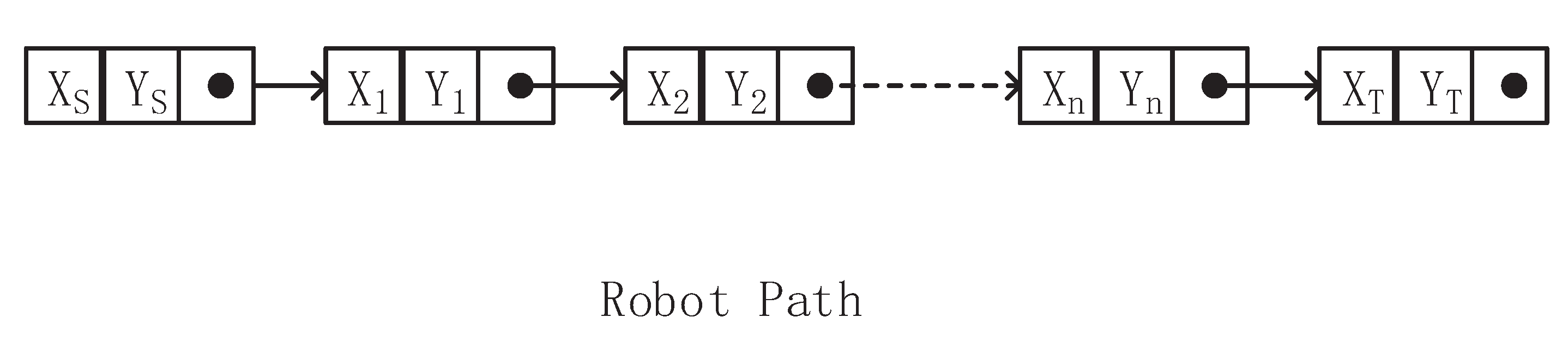
A path consists of successive segments. By summing all the segments of this path, the length of the entire path can be obtained. We assume that path contains a starting point (S), target point (T), and n consecutive points. The character (n) is the number of intermediate points or rotation points (RPs). Thus, a segment of path is generated by two consecutive points in the path. Figure 1 graphically represents the path.
3.1. Path Planning Objectives
In this work, to obtain precise and effective solutions, we optimized three objectives: path length, path safety and path smoothness.
The energy loss of a mobile robot is related to the length of the path—the longer the path, the greater the loss of energy. Besides the path length, the energy loss is also related to the smoothness of the path. For the same path length, the smoother the path, the smaller the energy loss. When the robot moves forward at a constant speed and only changes in velocity direction, the walking time of the robot is also related to the length. In addition, the most important factor that we need to consider is the safety of the path. The safe path distance reflects the distance from the surrounding obstacles—the greater the safety distance, the safer the path. So, this article describes the energy loss, walking time, and safety distance through the length, smoothness, and safety. We want to find the shortest, smoothest, and safest path. This is known as the multi-objective optimization problem. For the sake of convenience, we unified to minimize the three objectives. The mathematical definitions of these objectives are described in the following subsections.
3.1.1. Path Length
Based on the Euclidean distance, the segment length can be calculated between two consecutive points. By summing all the segments of this path, the length of the entire path can be obtained. represents path p. and denotes two consecutive points or rotation points (RPs). The length of a line segment is calculated using Equation (1):
A path consists of some consecutive segments, and the total length of path p can be calculated as follows:
3.1.2. Path Safety
The safe distance of the path reflects the distance from the surrounding obstacles. The set includes all m obstacles in the workspace. is the minimum distance between segment and obstacle . Therefore, is the shortest distance between the obstacles and the path—the larger the value, the safer the path. After adding a negative sign to the value, the maximum optimization safety problem is transformed into the minimum optimization problem. The path safety objective is calculated using Equation (3):
3.1.3. Path Smoothness
This is designed to calculate the degree of path bending. The smoother the path, the smaller the energy loss. The average angle of path represents the smoothness objective. The best average value is . This means that the path is straight.
For two consecutive segments and , , , the deviation angle is calculated with Equation (4):
In this work, for the path planning problem, the model of multi-objective optimization (MOP) is as follows:
A collision without obstacles is the only constraint. It is permissible to touch the boundaries of obstacles. In this work, we defined the infeasible path as a path to collide with obstacles and considered the boundary of the workspace as an obstacle.
Usually, at least two objectives conflict with each other. Approximate Pareto optimal paths can be found by solving the model illustrated in Equation (6). At present, many evolutionary algorithms have been able to solve lots of MOP problems, such as genetic algorithms, artificial bee colony algorithms, and particle swarm optimization algorithms. Although the MOP problem of path planning has been studied for many years, it is still difficult to efficiently find the approximate Pareto solutions due to the complexity of the path planning problem.
4. Multi-Objective Evolutionary Algorithm for the PP Problem
In this section, the proposed MOEA is clearly described. Chromosomes (or individuals) in MOEA move towards the global best solutions. Non-dominated individuals that have been discovered so far are clustered into a sub-group called the repository and converge to global non-dominated solutions. To further improve the local search capabilities, we propose a family of evolutionary operators for the population. We explain the algorithm in the following text.
4.1. Flow Chart
The flow chart of the proposed MOEA is as follows:
- (1)
- Initialize the population (POP).
- (2)
- Evaluate each individual in population (POP).
- (3)
- Store non-dominated individuals that have been found into the repository (REP).
- (4)
- The objective space that has been found is divided into grid regions, and the individuals of the repository (REP) are located in the corresponding grids.
- (5)
- While the number of iterations does not reach the preset maximum DO
- (a)
- Generate an empty population (NEWPOP): NEWPOP =
- (b)
- For to NP DO (%% NP is the number of chromosomes or individuals)(%% For individual POP[i], use refiner operators (safety, shortest, mutation, smoothness, shortness, and position update) to produce six new children. They are evaluated, and then, feasible individuals are placed in children population (NEWPOP). The feasible solution is one solution that lies on a valid search space. In this article, the feasible solution is one path that does not cross obstacles, but it can touch the boundaries of obstacles. If the new chromosome is an infeasible solution, replace the individual POP[i] with REP[h]. REP[h] is an individual repository and is chosen as follows: The more individuals in the grid, the lower the fitness values of these grids. This aims to decrease the possibility of selecting a grid with too many individuals. Then, based on the fitness values, roulette wheel selection is used to select the grid. Once a grid has been selected, we randomly consider an individual within this grid as REP[h]. The remainder operators are run for POP[i] in sequence. After the last operator (position update) has been used for the individual POP[i], if the generated children (co) are a feasible solution, replace POP[i] with co.
- (i)
- co = ClearanceOperator (POP[i])
- (ii)
- If IsInfeasibleSolution(co) doPOP[i] = REP[h]elseNEWPOP = NEWPOP + co
- (iii)
- Run the process (ii) with the remainder operators for POP[i] in sequence
- (iv)
- If IsFeasibleSolution(co) doPOP[i] = co
- (c)
- Update the contents of the repository (REP):REP = REP ∪ POP ∪ NEWPOP. Meanwhile, eliminate the dominating individuals in the repository (REP). Then, divide the found objective space into grid regions in step (4). Due to the limited capacity of the repository, when it is full, we remove individual REP[j] from the repository (REP) in turn until the number of individuals in the repository does not exceed the capacity of the repository. The following technique is used to select the individual REP[j]: The more individuals in the grid, the higher the fitness values of these grids. The aim is to increase the possibility of selecting a grid with too many individuals. Then, based on the fitness values, roulette wheel selection is used to select the grid. Once a grid has been selected, we randomly consider an individual within this grid as REP[j].
- (d)
- Increment the loop counter.
In the proposed algorithm, each individual is a path and the path consists of a number of sequential segments. Therefore, the feasibility of individual is determined by the feasibility of the path. As we can see, the algorithm starts from initialization steps 1–4. Once the initialization steps have been finished, the algorithm iterates (considering the maximum number of iterations) and attempts to find the best solutions by repeating step 5. At the beginning of each iteration, an empty children population (NEWPOP) is generated, and a family of operators is applied to each individual POP[i]. The new individuals are produced and feasible solutions of them are inserted into the children population (NEWPOP). Then, the repository (REP) is updated (REP = REP ∪ POP ∪ NEWPOP). In this update, the dominated solutions are discarded, and the non-dominated solutions are stored until the maximum allowed capacity of repository (REP) is reached. The process of 5_(c) guarantees that the obtained well-distributed Pareto front is not destroyed.
In addition, some evolutionary operators are shown to find the feasible and optimal paths more efficiently. Six operators (safety, shortest, mutation, smoothness, shortness, and position update) are presented. In this article, we select three well-known objectives (path length, safety, and smoothness) to optimize. Six operators are proposed to optimize the three corresponding objectives. The safety operator is used to increase the safety of a path. The shortest and shortness operators are used to shorten the path length differently. The mutation is used to randomly change the RPs of a path. The smoothness operator attempts to get as smooth of a path as possible. The position update operator is designed to change the RPs of the path by using the positions of the RPs. Therefore, the six operators are related to the three objectives that need to be optimized. All of the operators use probability. We clearly explain the initialization and operators in the following text.
4.2. Safety Operator
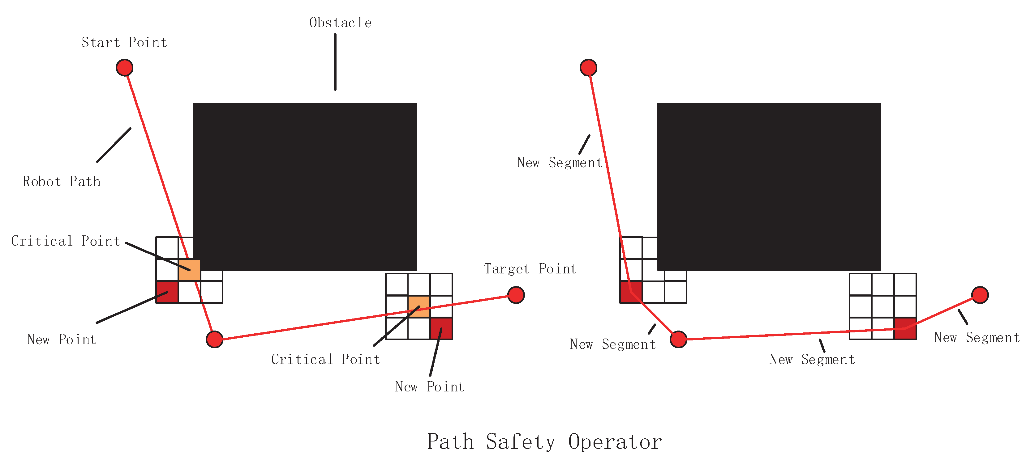
The safety operator attempts to increase the safety of the path. Each segment is regarded as an input, and in turn, we attempt to increase the safe distance between the segment and the obstacles. Let us first define the critical point.
The critical point is the closest point on the segment to the obstacles. We find the critical point and replace it with a newly generated free point near the critical point to give a greater safety distance. The new point is generated by dividing the workplace into grid regions. In this work, we set the number of grids to . The grid () that the critical point is located in and the center points of the adjacent 8 grids of are found. The safety distances of the 8 center points and the critical point are compared, and then one point that has the maximum safety value is selected as the new point. Note that when all segments of this path have been handled with the safety operator, the operator is finished. Figure 2 illustrates the safety operator.
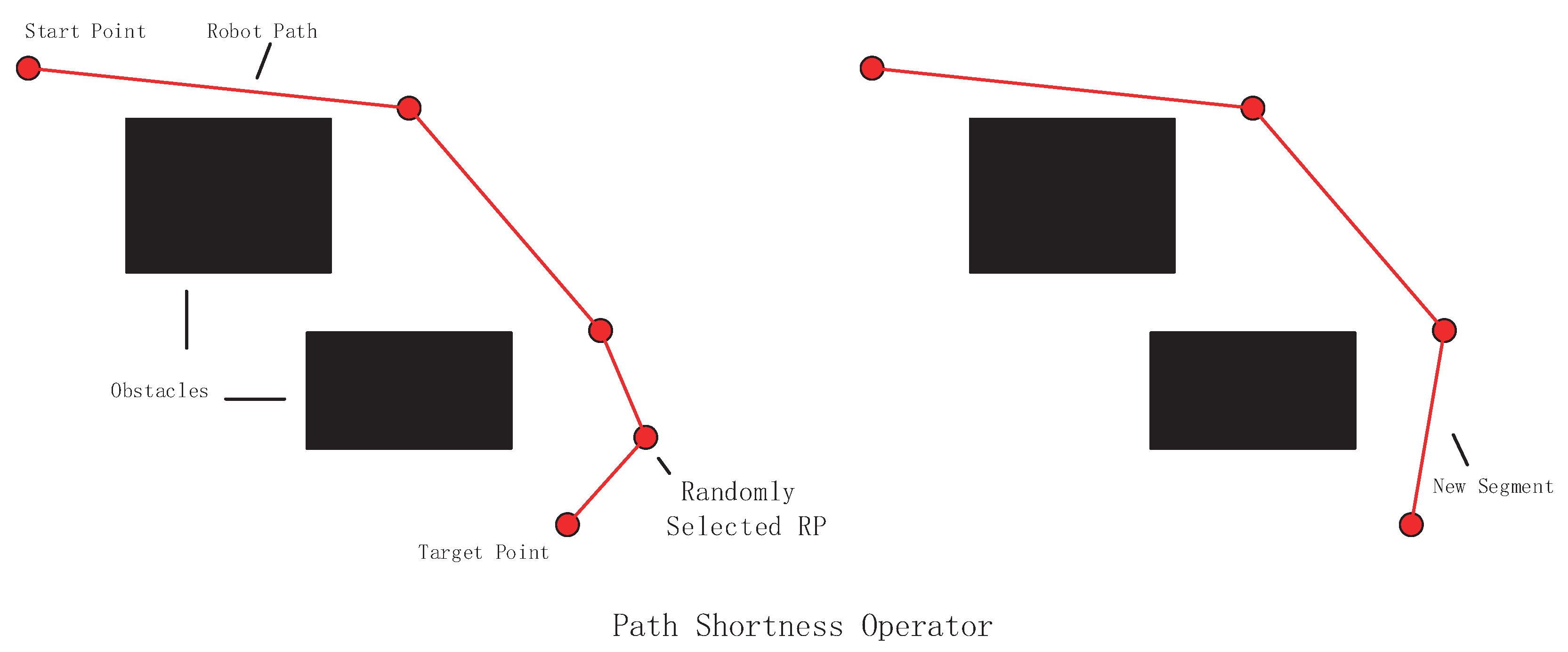
4.3. Shortest Operator
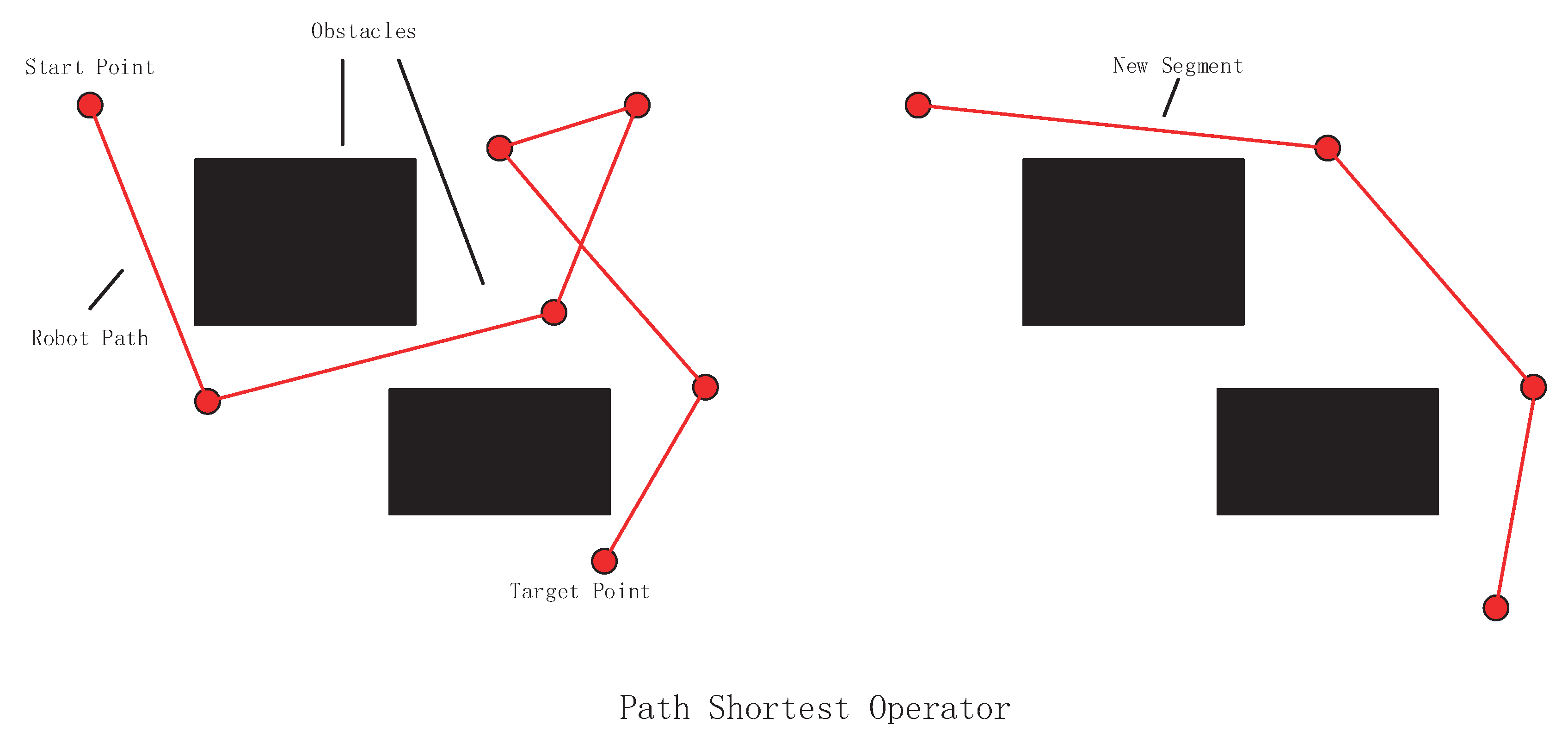
When the speed of the mobile robot is constant and only the direction changes, the walking time of the robot is related to the path length. Therefore, the shorter the path length is, the shorter the walking time of the robot is. The shortest operator aims to remove the extra rotation points (RPs) on the path and reduce the length of path. For the i-th rotation point in the path, the j-th point is selected in turn from the target point (T) to the (-th point. If the new segment () does not collide with the obstacles, the points between the i-th and j-th points in the path are deleted. The iteration runs if the value of i satisfies the following condition: . n is the number of RPs on the path. The shortest operator can obtain a new feasible path. This operator has a powerful force for finding the shortest path. To avoid premature convergence to a local optimal solution, the probability of the shortest operator is set to . Figure 3 presents the shortest operator.
4.4. Mutation Operator
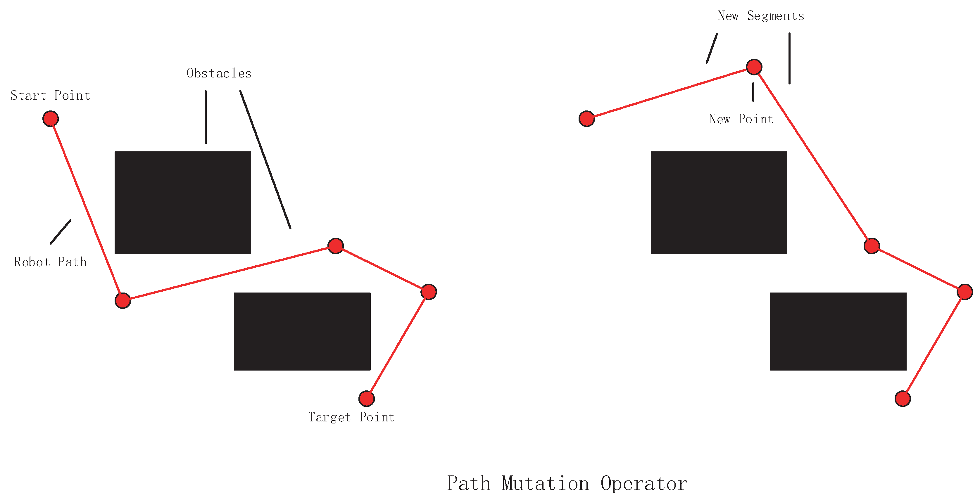
The mutation operator randomly modifies a rotation point on the path. The process of mutation is that a rotation point is randomly selected, and then it is replaced with a random point in free space. Figure 4 shows the mutation operator.
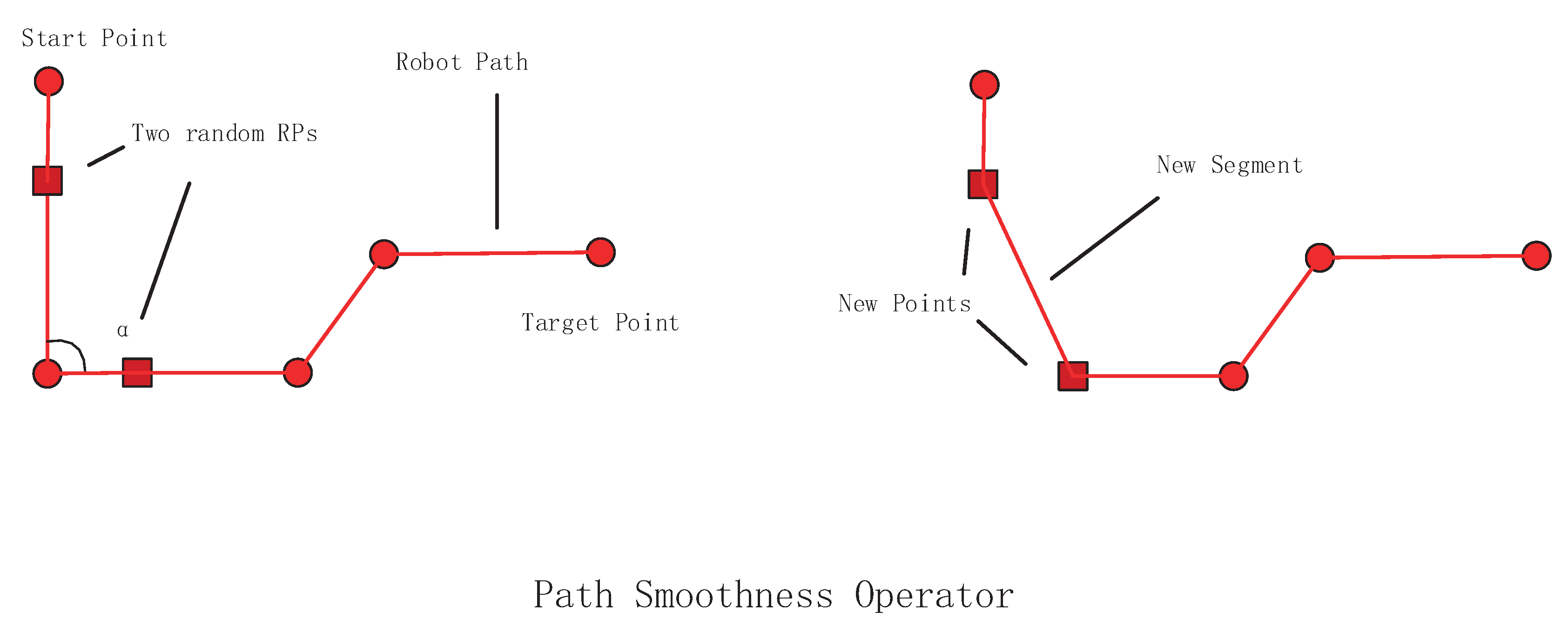
4.5. Smoothness Operator
For the same length path, the smoother the path is, the lower the energy consumption is. Therefore, smoothness is also one of the factors that affects energy loss. The smoothness operator aims to find a path—the smoother the better. It reduces the maximum turn angle to improve it. First, we find the maximum turn angle and the two line segments that generate the angle. Each of the two segments randomly generates a free point. We take the two newly generated points as the rotation points, and then remove the intersection points of the two line segments. Accordingly, the maximum turn angle of the new path reduces. The smoothness operator is shown in Figure 5.
4.6. Shortness Operator
The shortness operator is designed to randomly decrease the path length. It randomly removes a rotation point on the path. This means that the previous point and the next point form a new line segment. It deletes two line segments and adds a shorter line segment to the path. Apparently, the whole length of the path decreases. In addition, this operator is different from the shortest operator. This operator uses a mechanism which randomly deletes a point on the path and may generate a new path that is not feasible. However, the shortest operator does not change the feasibility of the path. A graphical explanation of the shortness operator is shown in Figure 6.
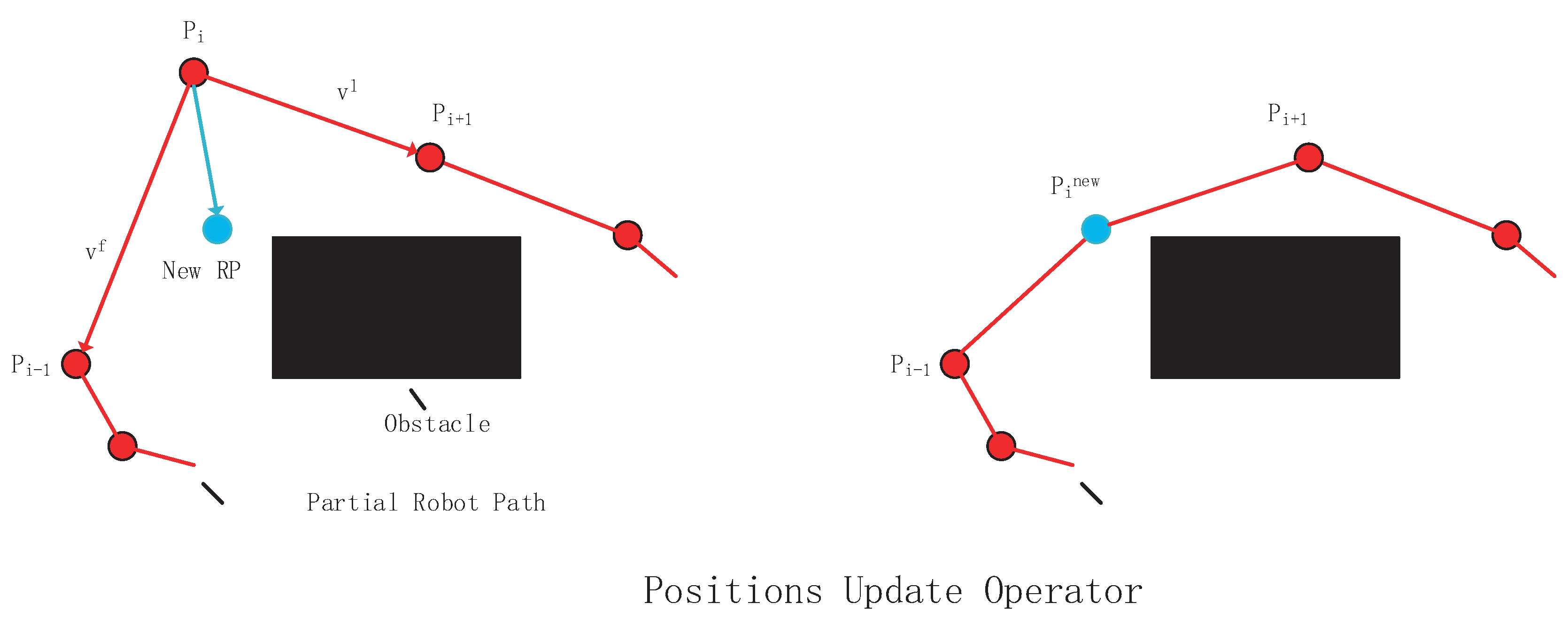
4.7. Position Update Operator
This operator aims to improve a path by utilizing consecutive rotation points. A path () contains a starting point (S), a target point (T), and n rotation points. Based on the position and velocity of rotation point (), a new rotation point () can be acquired with Equation (7): . The general mechanism of the position update operator is presented in Figure 7.
The generated velocity (v) should satisfy the constraint . In other words, the vector of v should be located in the rectangular region generated by the minimum velocity () and maximum velocity (). Furthermore, the newly generated rotation point () should be in the free workspace. If point () is not feasible, its new value is adjusted with Equation (8) until point () is feasible. Since new segments may collide with obstacles, we should examine the feasibility of the two new segments () and (). If there is a collision, the position of rotation point () needs to be adjusted with Equation (8). In this operator, , , and are random numbers ranging from 0 to 1:
4.8. Initialization
Generally, generating an initial population is always the first step of evolutionary algorithms. Potential solutions (individuals) are generated and evolved. The individual in the population is a random path. Each path consists of k random rotation points in the free workspace. k is a random number ranging from 1 to 3. The number of rotation points on the path varies after using evolutionary operators.
Three objectives (length, safety, and smoothness) were optimized in this article. To further improve the evolutionary efficiency, we found the local minimum value of each objective (if it could be found) and put the corresponding feasible paths into the initial population. For the length and safety of path, we provide the following two ideas to find the local minimum feasible paths. In regard to the smoothness objective of the path, the local minimum smooth path exists in the region near the local minimum distance path or the local minimum safety path, so improvements in the local minimum distance and safety of the paths were sufficient.
For the path length, we used the Dijkstra algorithm to find the local minimum distance path, as follows: (1) Find the set (Q) of obstacles that collide with the line segment (). (2) For each obstacle (j; ), if the line segment between any vertex of j and the start point (S) collides with obstacle k (), or the line segment between any vertex of j and the target point (T) collides with obstacle k (), obstacle k is put into set Q. (3) For each obstacle (j; ), all vertices are stored into set . (4) For any two vertices (; ), if the line segment () is located in the semi-free space, the line segment () is put into the edges set (). (5) For all vertexes () and edges (), the local minimum length path can be obtained with the Dijkstra algorithm.
Next, we show how to find the local minimum safety path. This idea is inspired by dividing the continuous workspace into discrete grids, as follows. (1) First, divide the workspace into grids, calculate the clearance distance of each grid from corresponding nearest obstacles, and convert the clearance distance into a safety value—the closer to the obstacle, the greater the safety value is. Conversely, the farther away from the barrier, the smaller the safety value is. (2) Taking into account the safety values of all grids and the four-connected relationship (namely, each grid has 4 adjacent grids), the Dijkstra algorithm can be used to find the local minimum safety path from the start grid (where the start point is located) to the target grid (where the target point is located). (3) If the local minimum safety path does not exist or the path is not feasible, the number (N) of grids is increased and we go back to step (1). Note that the initial grids (N) can be set to a small value, such as 400, and then the value of N is gradually increased.
Finally the parameters are set as follows. The size of population is set to 80. The maximum generation number is set to 100. The size of repository is set to 300. The objective search space is divided into grid regions. In addition, we set the probabilities of safety, shortest, mutation, smoothness, shortness, and positions update operators to , , , , , , respectively. Furthermore, the velocity constraints in the position update operator are set to of the vector distance between the upper boundary and lower boundary of the workspace.
5. Results
In this section, we compare MOEA with PSO. PSO was used in article [30] to solve the PP problem. In order to compare the characteristics of algorithms, we used different quality metrics including the hypervolume indicator (HV) [43] and the set coverage metric (scm) [44].
In the objective space, the volume of non-dominated solutions can be measured by the HV. We first define the concepts of characters. Non-dominated solutions are denoted by . The reference point is represented by . In the d-objective minimum optimization problem, the hypervolume region of A restricted by r can be calculated with Equation (9). L represents the Lebesgue measure [45]:
Therefore, the dominant proportions of two groups of non-dominated solutions can be measured by the set coverage metric (scm). The two groups of solutions are denoted by and , respectively. Accordingly, can be shown as
If , any solution in A is better than the solution in B. On the contrary, if , this implies that any solution in B is better than the solution in A. Since relationship (⪯) denotes a weak dominance relation and is not symmetric, and need to be calculated. In other words, the sum of them is not definitely equal to 1.
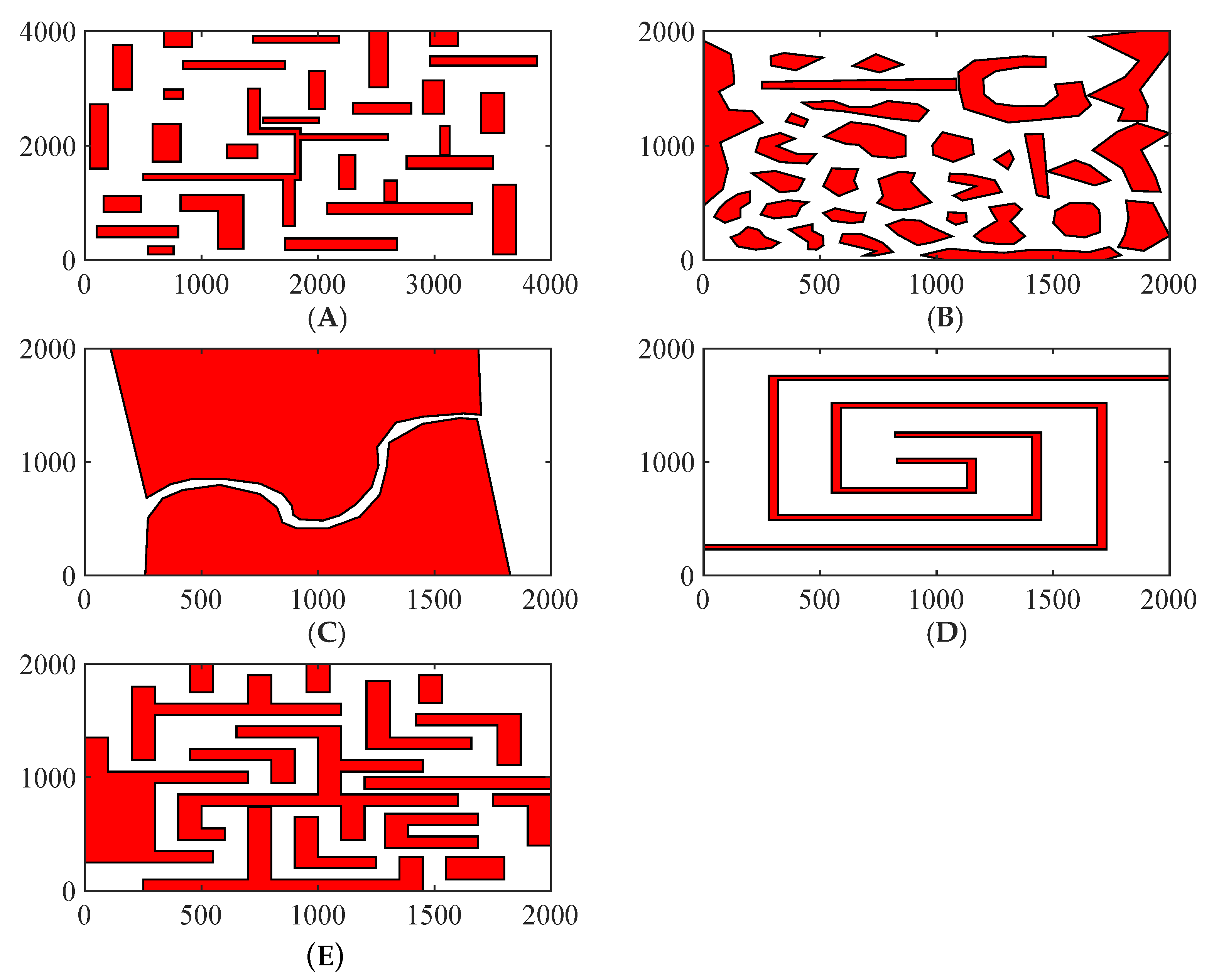
The five scenarios shown in Figure 8 were used for testing. More maps are available from http://imr.ciirc.cvut.cz/planning/maps.xml. In each workspace, obstacles were generated. The starting point and target point are presented in Table 1. For equitable contrast, the following PSO parameters were set: the swarm size was 80, the maximum generation number was 100, the size of the feasible archive was 20, and the size of the infeasible archive was 20, and the maximal sampling times was 20, respectively. For each scenario shown in Figure 8, 30 independent runs were performed. In each run, the optimal solutions obtained by two algorithms were analysed with quality metrics. Table 2 presents the results of the hypervolume median and interquartile range. The results show that the solutions obtained by MOEA were larger and denser in objective space.
Furthermore, set coverage metric (scm) was also used to test the solutions. The results are presented in Table 3. It is obvious that most of solutions obtained by MOEA dominated the solutions by PSO. The average value of scm (MOEA, PSO) was , while the average value of scm (PSO, MOEA) was . The results indicate that solutions obtained by MOEA are closer to the approximate Pareto front.
Moreover, in each scenario, we needed to use reference points. The ideal reference point should be the ideal optimal value of objectives and is defined as the following. The ideal minimum length can be calculated by linking the starting point and target point with a line segment. In a similar manner, the ideal smoothness value is equal to 0. Since the safety is not positive, the smaller the value is, the safer the path is. The ideal safety value is computed by adding to the minimum safety value. On the contrary, the nadir reference point is the nadir worst value of objectives. For the length and smoothness objectives, the nadir worst values are computed by adding to the worst values. We set the worst safety value to 0; this value implies that the path touches the boundary of obstacles and does not collide with obstacles. The reference points are presented in Table 4.
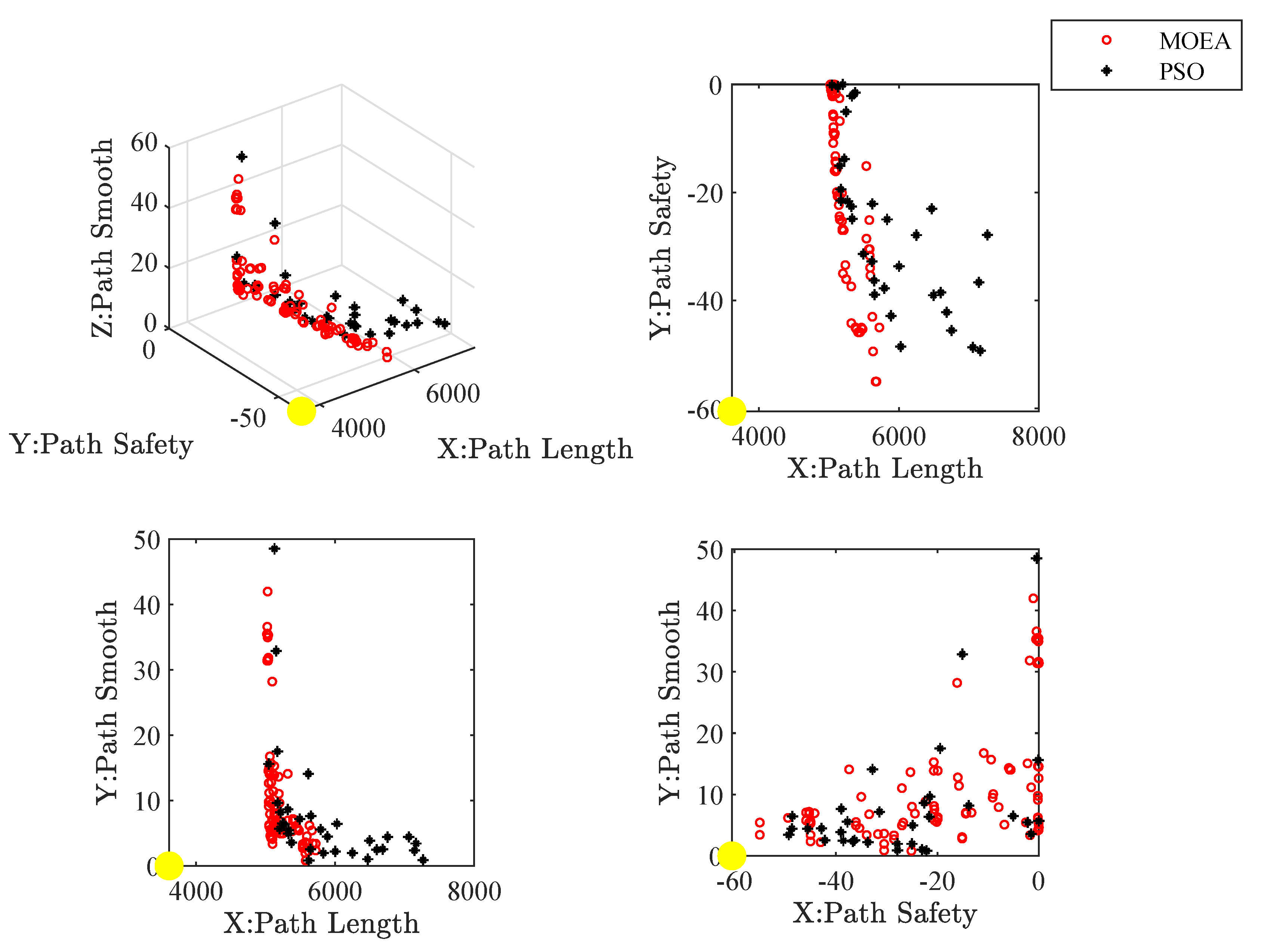
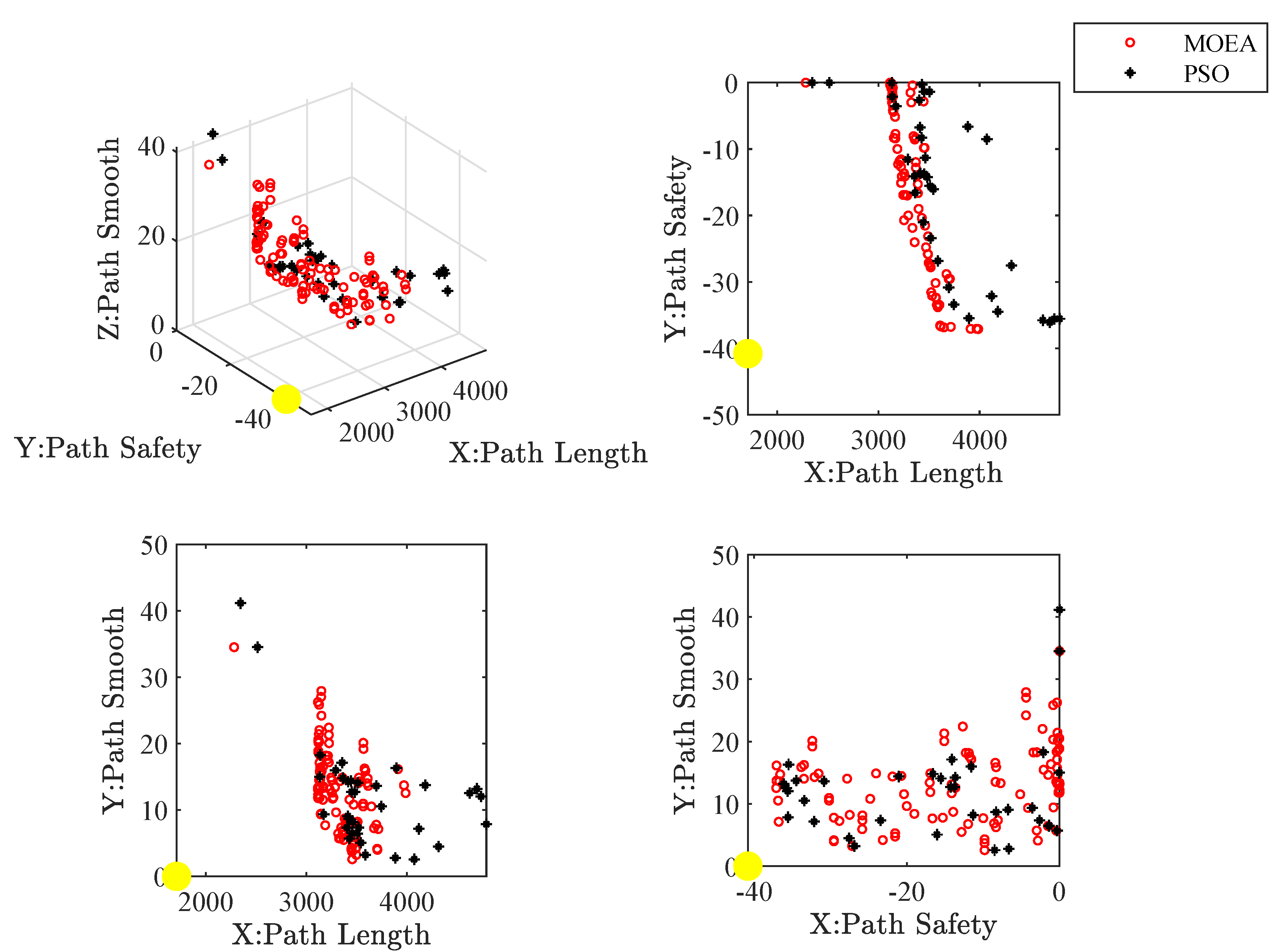
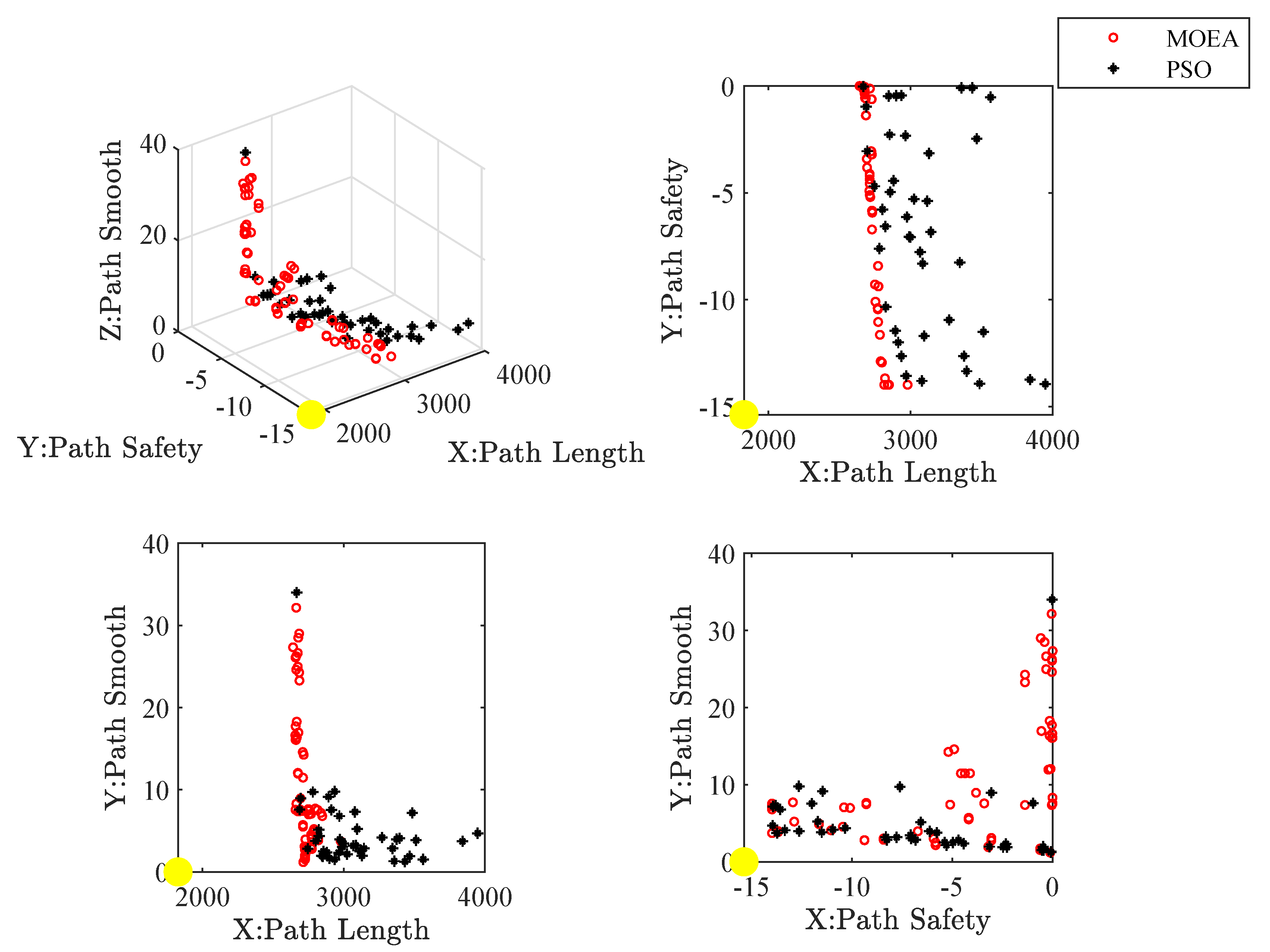
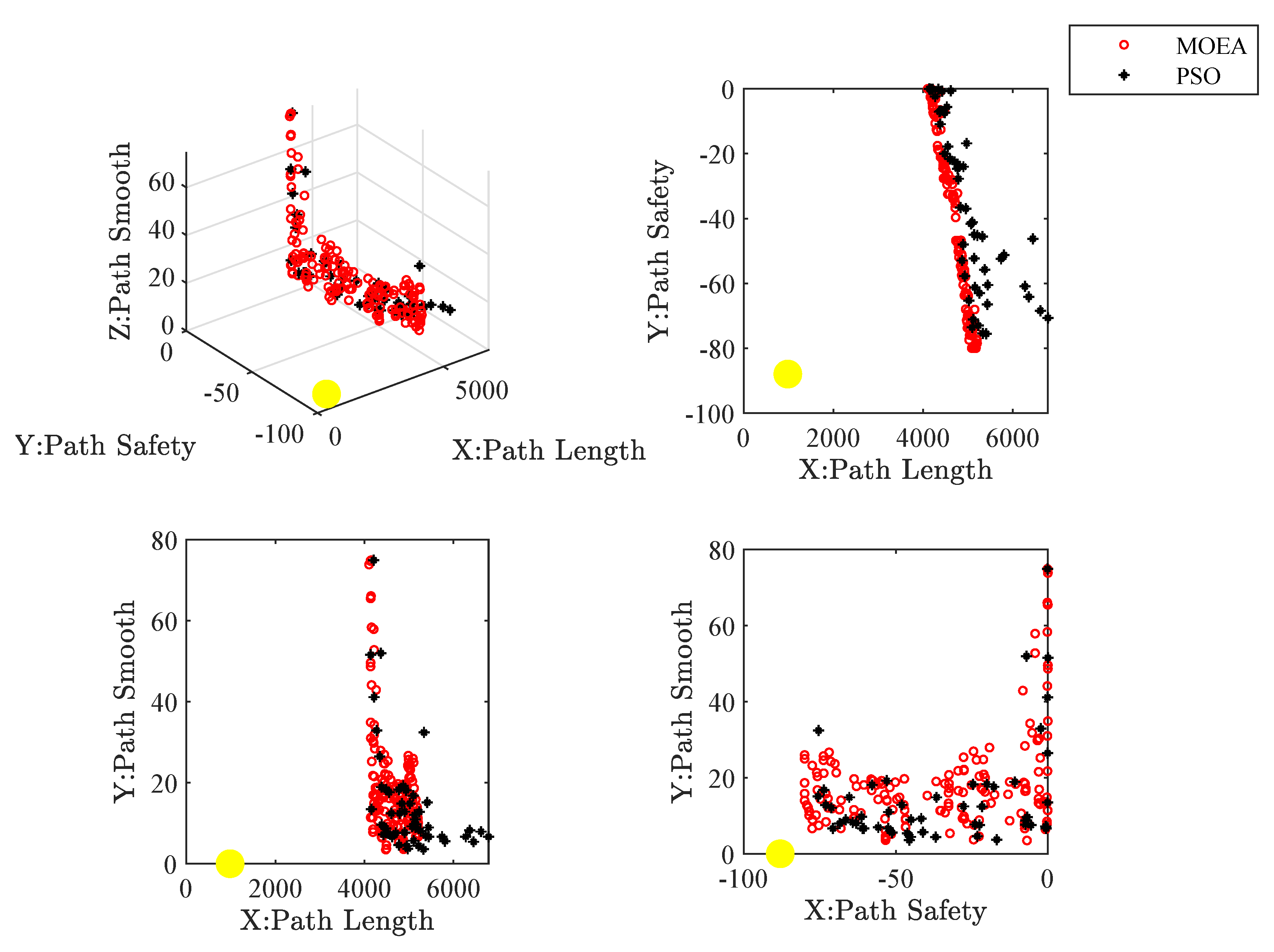
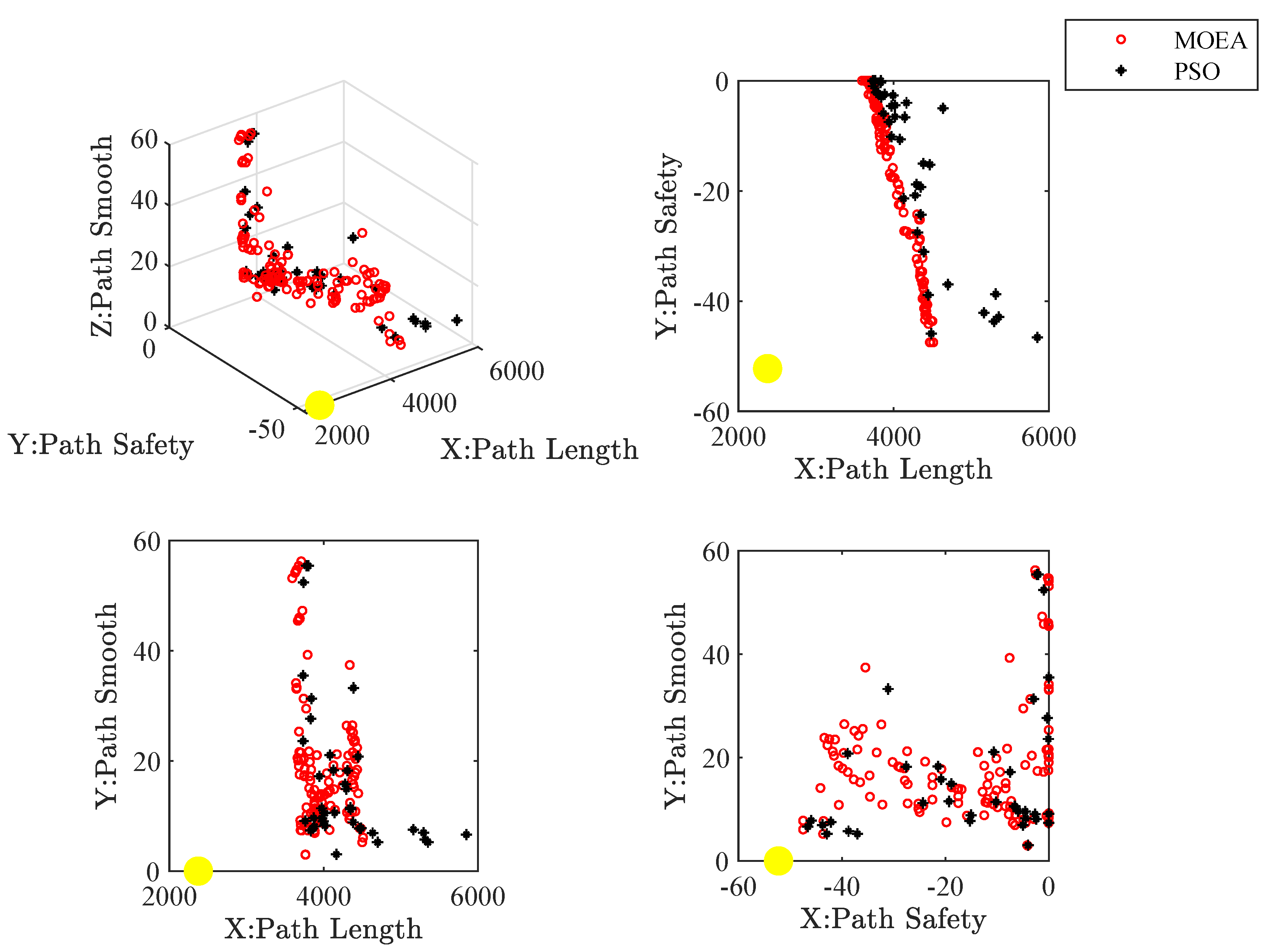
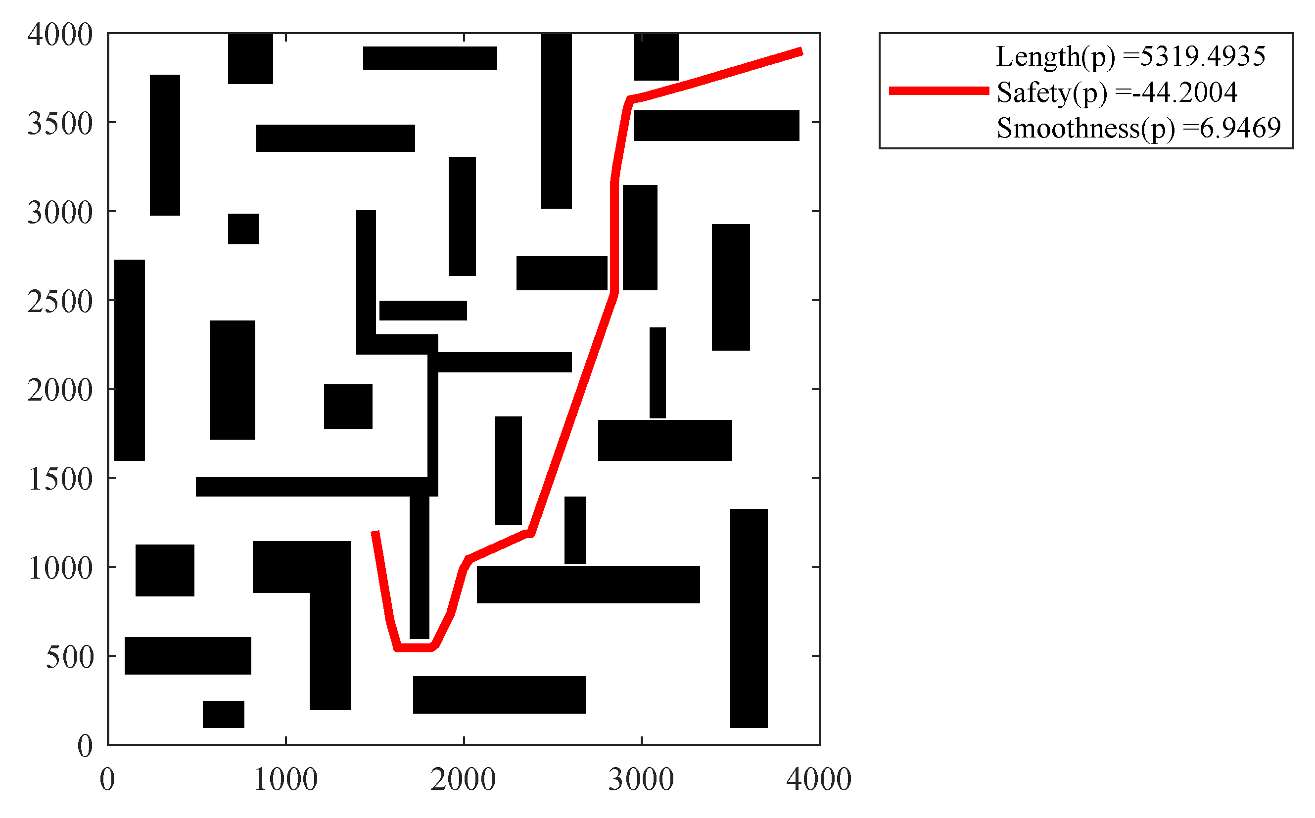
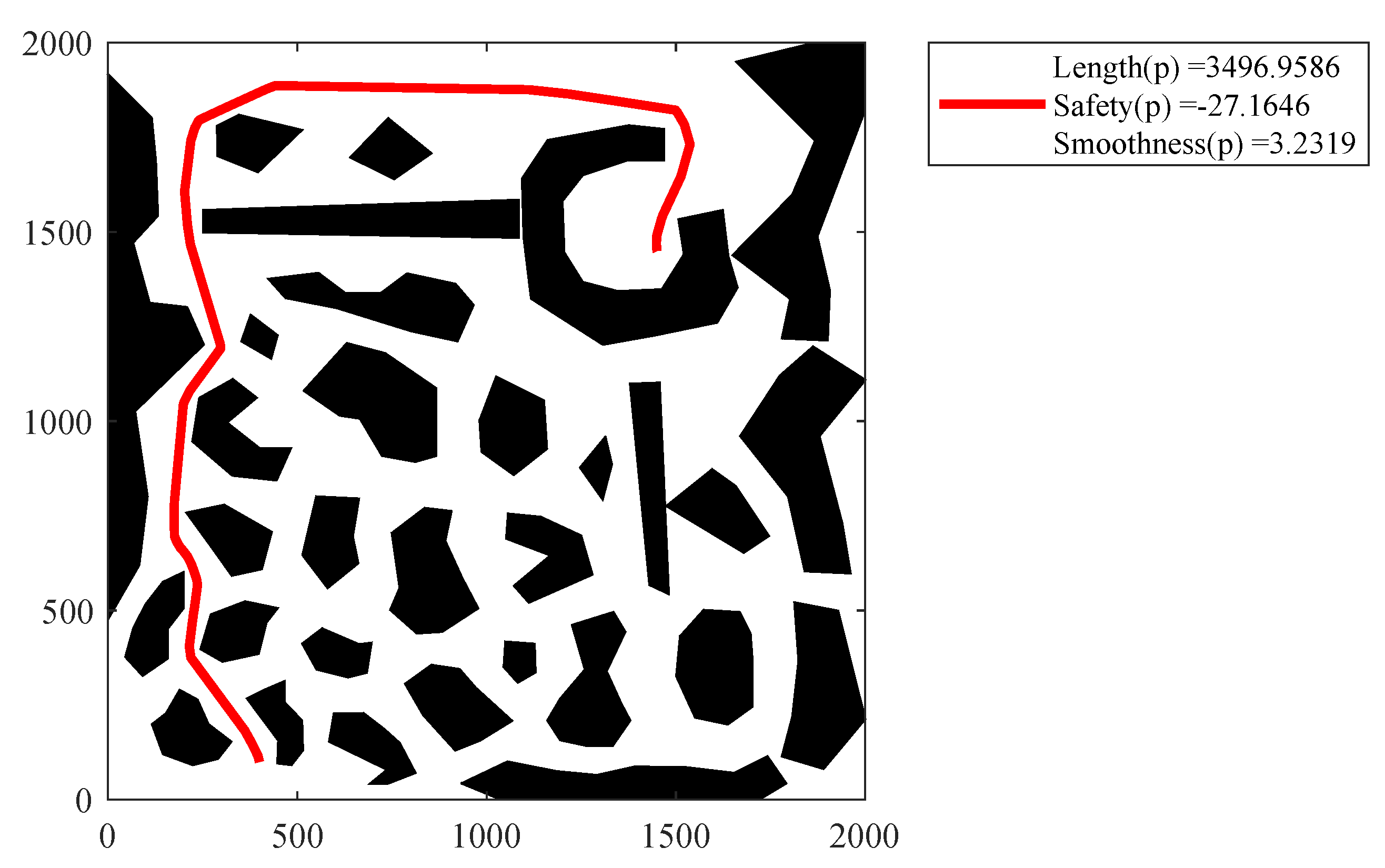
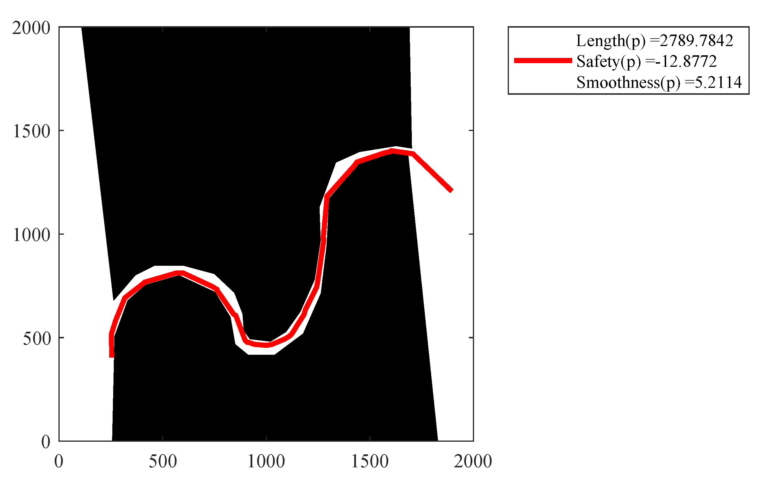
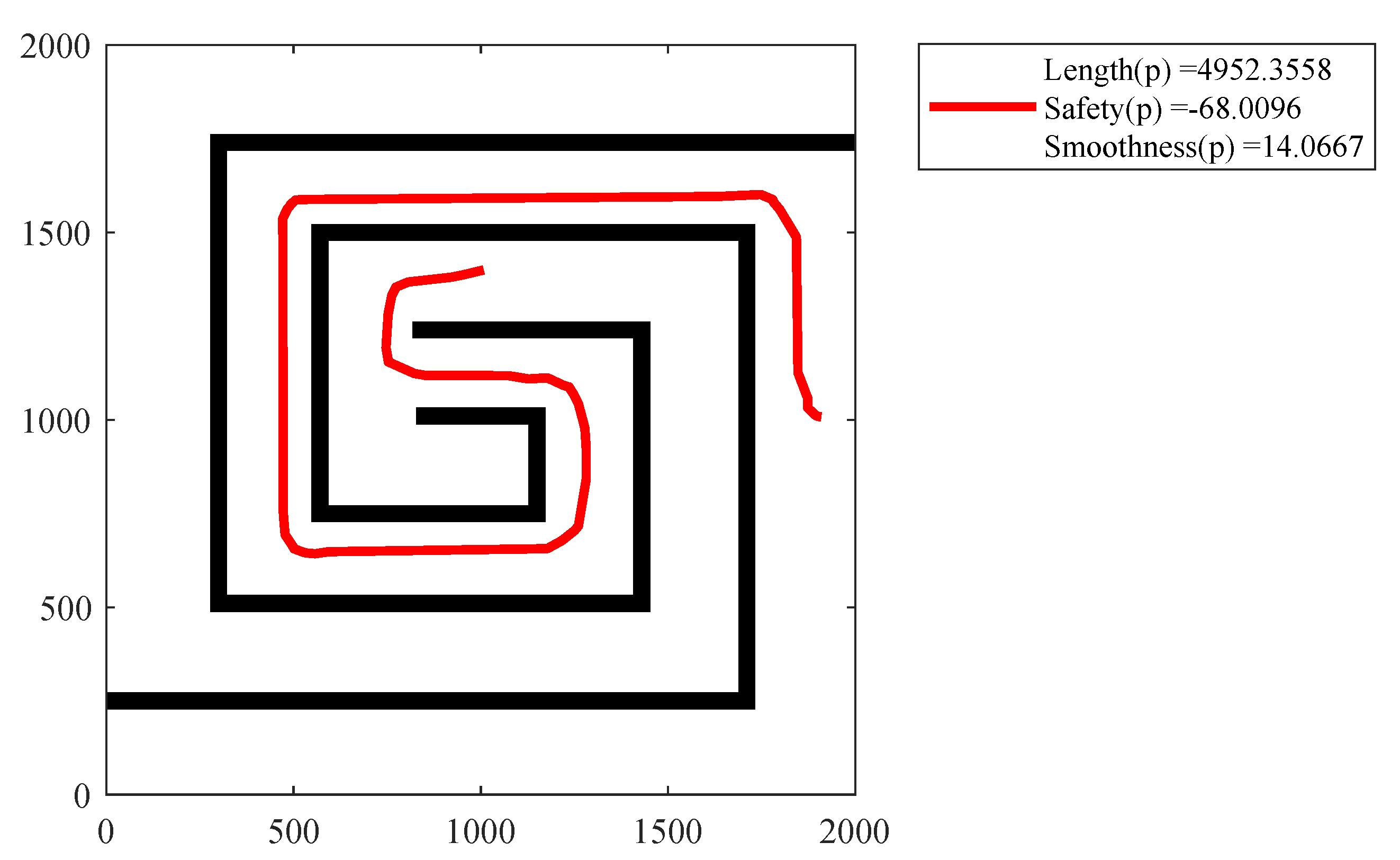
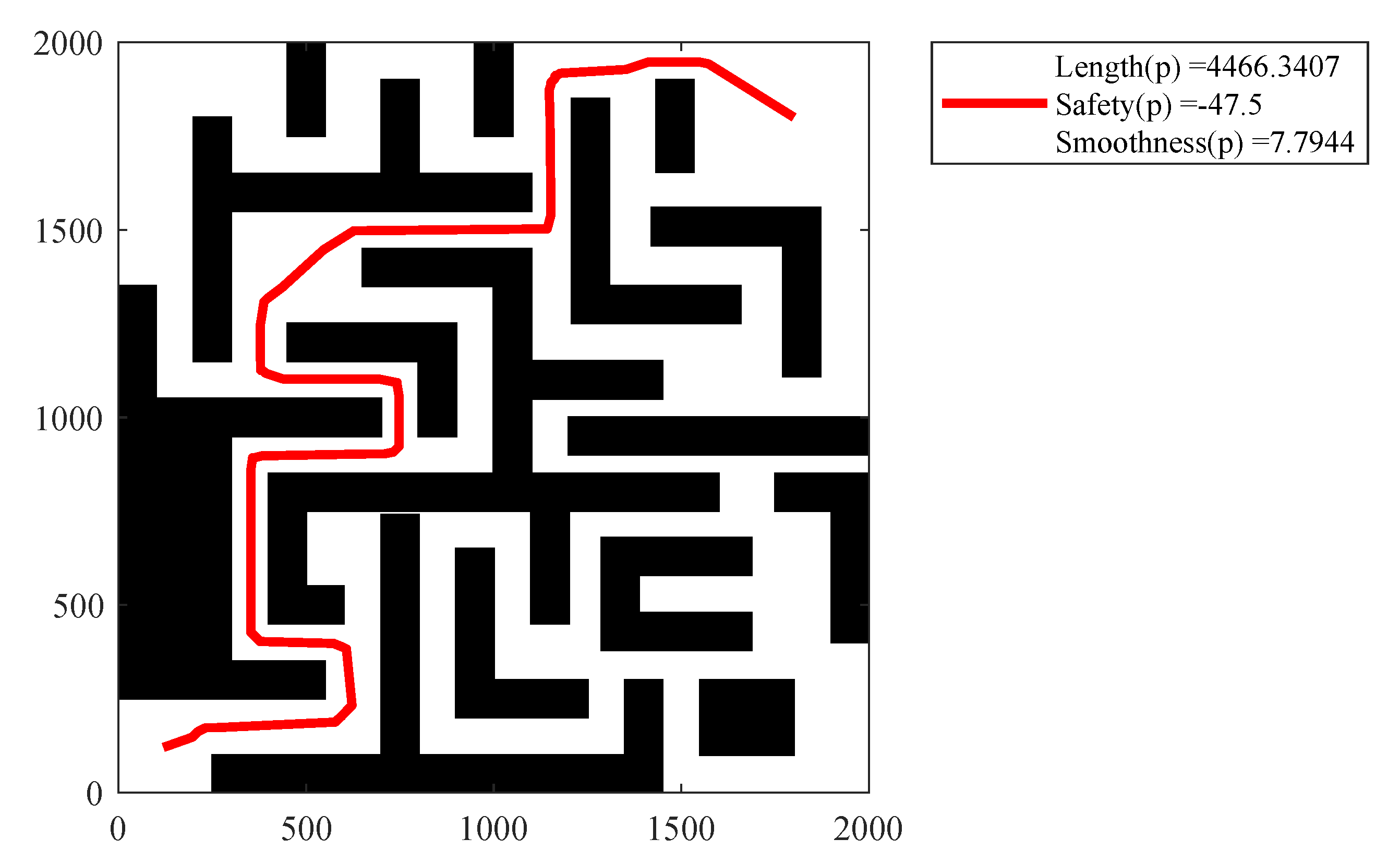
For the five scenarios shown in Figure 8, Figure 9, Figure 10, Figure 11, Figure 12 and Figure 13 show the approximate Pareto front. The red circles represent the non-dominated solutions with the proposed MOEA algorithm. It is clear that red circles are closer to the yellow ideal point than the black points. The black points denote the solutions with PSO. This also indicates that solutions by MOEA are closer to the approximate Pareto front. Moreover, the best paths are presented in Figure 14, Figure 15, Figure 16, Figure 17 and Figure 18. The best path is a solution and has the minimum distance from the ideal point. The objectives were normalized and the distances were calculated with the Euclidean distance.
The following insights can be emphasized from the experimental results. For the multi-objective PP problem, MOEA has a better set coverage metric than PSO. This means that MOEA can obtain better quality solutions (optimizing three objectives: path length, safety, and smoothness).
6. Conclusions and Future Work
In this article, MOEA was presented to resolve the path planning problem. We dealt with three objectives: length, safety, and smoothness. In addition, we also proposed extra evolutionary operators to find precise and effective paths. Moreover, we used the well-known PSO algorithm for comparison. The obtained results were evaluated with the hypervolume indicator (HV) and the set coverage metric (scm). The comparisons show that the solutions obtained by MOEA are larger and denser in objective space and closer to the approximate Pareto front. Accordingly, five different scenarios were used for testing. The results show the advantages of proposed MOEA. This is a significant contribution. Another contribution is that we combine the advantages of the evolutionary algorithm with the traditional heuristic Dijkstra method to further improve the search efficiency.
The shortcomings in this work are as following: (1) Since the operators are not very fast, the algorithm is currently only suitable for the off-line path planning problem. The next step is to further improve the computing speed of the operators. (2) Because the proposed algorithm does not consider the size and dynamic behavior of a specific robot, the algorithm can only plan the optimal path for the mobile robot. Other work can then be carried out, such as trajectory tracking.
In the field of path planning, there are still many issues that are worthy of attention. For the single-objective path planning problems, at present, some scholars are focused on the following topics: (1) More efficient algorithms are needed to solve large-scale and real-time path planning problems. (2) Based on the dynamic characteristics of robots, by controlling the behavior of the robot motor in real time, the path planning problem and the trajectory tracking problem are combined to find an optimal walking path. For multi-objective path planning problems, there are several problems that need to be solved: (1) Most algorithms designed by scholars are offline. It is a challenging task to improve the computational efficiency of the algorithms. Hybrid algorithms may be effective approaches. (2) Currently, several researchers are focused on the dynamic environment. There are three types of dynamic obstacles: (a) The positions and velocities of the dynamic obstacles at any one time are completely known; (b) the positions and velocities of the dynamic obstacles are unknown, but predictable; and (c) the positions and velocities of the dynamic obstacles are unknown and unpredictable. There are some heuristic algorithms such as D* lite that can solve the single-objective shortest path in dynamic environments. For multi-objective path planning problems in dynamic environments, it may be a good solution to combine evolutionary algorithms with the advantages of traditional heuristic algorithms. (3) In recent years, some scholars have focused on the multi-robot multi-objective path planning problem. This is a complex coupling optimization problem. We will continue to focus on and solve these issues over the next few years.
Author Contributions
Y.X. investigated the relevant literature, proposed and implemented the algorithm, and wrote the paper; J.-Q.S. provided resources, confirmed the feasibility of the algorithm and revised the article.
Funding
This research received no external funding.
Conflicts of Interest
The authors declare no conflicts of interest.
Abbreviations
| PP | Path planning |
| MOEA | Multi-objective evolutionary algorithm |
| MOP | Multi-objective optimization |
| PSO | Particle swarm optimization |
| RP | Rotation point |
| HV | Hypervolume |
| scm | Set coverage metric |
References
- Algfoor, Z.A.; Sunar, M.S.; Kolivand, H. A comprehensive study on pathfinding techniques for robotics and video games. Int. J. Comput. Games Technol. 2015, 2015, 7. [Google Scholar] [CrossRef]
- Choset, H.M. Principles of Robot Motion: Theory, Algorithms, and Implementation; The MIT Press: Cambridge, MA, USA, 2005. [Google Scholar]
- LaValle, S.M. Planning Algorithms; Cambridge University Press: Cambridge, UK, 2006. [Google Scholar]
- Alomari, A.; Phillips, W.; Aslam, N.; Comeau, F. Swarm intelligence optimization techniques for obstacle-avoidance mobility-assisted localization in wireless sensor networks. IEEE Access 2017, 99, 22368–22385. [Google Scholar] [CrossRef]
- Alomari, A.; Phillips, W.; Aslam, N.; Comeau, F. Dynamic fuzzy-logic based path planning for mobility-assisted localization in wireless sensor networks. Sensors 2017, 17, 1904. [Google Scholar] [CrossRef] [PubMed]
- Chen, Y.; Lu, S.; Chen, J.; Ren, T. Node localization algorithm of wireless sensor networks with mobile beacon node. Peer-to-Peer Netw. Appl. 2017, 10, 795–807. [Google Scholar] [CrossRef]
- Mohanan, M.G.; Salgoankar, A. A survey of robotic motion planning in dynamic environments. Robot. Auton. Syst. 2018, 100, 171–185. [Google Scholar] [CrossRef]
- Madkour, A.; Aref, W.G.; Rehman, F.U.; Rahman, M.A.; Basalamah, S. A survey of shortest-path algorithms. arXiv, 2017; arXiv:1705.02044. [Google Scholar]
- Redlarski, G.; Dabkowski, M.; Palkowski, A. Generating optimal paths in dynamic environments using River Formation Dynamics algorithm. J. Comput. Sci. 2017, 20, 8–16. [Google Scholar] [CrossRef]
- Patle, B.K.; Parhi, D.R.K.; Jagadeesh, A.; Kashyap, S.K. Matrix-Binary Codes based Genetic Algorithm for path planning of mobile robot. Comput. Electr. Eng. 2017, 67, 708–728. [Google Scholar] [CrossRef]
- Pandey, A.; Parhi, D.R. Optimum path planning of mobile robot in unknown static and dynamic environments using Fuzzy-Wind Driven Optimization algorithm. Def. Technol. 2017, 13, 47–58. [Google Scholar] [CrossRef]
- Hart, P.E.; Nilsson, N.J.; Raphael, B. A formal basis for the heuristic determination of minimum cost paths. IEEE Trans. Syst. Sci. Cybern. 1968, 4, 100–107. [Google Scholar] [CrossRef]
- Stentz, A. Optimal and efficient path planning for partially-known environments. In Proceedings of the IEEE International Conference on Robotics and Automation, San Diego, CA, USA, 8–13 May 1994; pp. 3310–3317. [Google Scholar] [Green Version]
- Silva, J.B.; Siebra, C.A.; do Nascimento, T.P. A New Cost Function Heuristic Applied to A* Based Path Planning in Static and Dynamic Environments. In Proceedings of the 12th Latin American Robotics Symposium and Third Brazilian Symposium on Robotics, Uberlândia, Brazil, 28 October–1 November 2015; pp. 37–42. [Google Scholar]
- Xu, J.; Gao, Y.; Liu, C.; Zhao, L.; Ding, Z. Efficient route search on hierarchical dynamic road networs. Distrib. Parallel Databases 2015, 33, 227–252. [Google Scholar] [CrossRef]
- Ammar, A.; Bennaceur, H.; Châari, I.; Koubâa, A.; Alajlan, M. Relaxed Dijkstra and A* with linear complexity for robot path planning problems in large-scale grid environments. Soft Comput. 2016, 20, 4149–4171. [Google Scholar] [CrossRef]
- Cao, P.; Fan, Z.; Gao, R.X.; Tang, J. Design for Additive Manufacturing: Optimization of Piping Network in Compact System with Enhanced Path-Finding Approach. J. Manuf. Sci. Eng. 2018, 140, 081013. [Google Scholar] [CrossRef]
- Dang, V.H.; Thang, N.D.; Viet, H.H.; Tuan, L.A. Batch-Theta* for path planning to the best goal in a goal set. Adv. Robot. 2015, 29, 1537–1550. [Google Scholar] [CrossRef]
- Canny, J. The Complexity of Robot Motion Planning; The MIT Press: Cambridge, MA, USA, 1988. [Google Scholar]
- Elshamli, A.; Abdullah, H.A.; Areibi, S. Genetic algorithm for dynamic path planning. In Proceedings of the Electrical and Computer Engineering, Niagara Falls, ON, Canada, 2–5 May 2004; pp. 677–680. [Google Scholar]
- Chen, X.; Li, Y. Smooth path planning of a mobile robot using stochastic particle swarm optimization. In Proceedings of the IEEE International Conference on Mechatronics and Automation, Luoyang, China, 25–28 June 2006; pp. 1722–1727. [Google Scholar]
- Mandow, L.; De La Cruz, J.L.P. Multiobjective A* search with consistent heuristics. J. ACM 2010, 57, 27. [Google Scholar] [CrossRef]
- Lavin, A. A pareto optimal D* search algorithm for multiobjective path planning. arXiv, 2015; arXiv:1511.00787. [Google Scholar]
- Oral, T.; Polat, F. MOD* Lite: An incremental path planning algorithm taking care of multiple objectives. IEEE Trans. Cybern. 2016, 46, 245–257. [Google Scholar] [CrossRef] [PubMed]
- Contreras-Cruz, M.A.; Ayala-Ramirez, V.; Hernandez-Belmonte, U.H. Mobile robot path planning using artificial bee colony and evolutionary programming. Appl. Soft Comput. 2015, 30, 319–328. [Google Scholar] [CrossRef]
- Chen, X.; Kong, Y.; Fang, X.; Wu, Q. A fast two-stage ACO algorithm for robotic path planning. Neural Comput. Appl. 2013, 22, 313–319. [Google Scholar] [CrossRef]
- Ghatee, M.; Mohades, A. Motion planning in order to optimize the length and clearance applying a Hopfield neural network. Expert Syst. Appl. 2009, 36, 4688–4695. [Google Scholar] [CrossRef]
- Châari, I.; Koubâa, A.; Bennaceur, H.; Ammar, A.; Trigui, S.; Tounsi, M.; Shakshuki, E.; Youssef, H. On the adequacy of tabu search for global robot path planning problem in grid environments. Procedia Comput. Sci. 2014, 32, 604–613. [Google Scholar] [CrossRef]
- Gong, D.-W.; Zhang, J.-H.; Zhang, Y. Multi-objective particle swarm optimization for robot path planning in environment with danger sources. J. Comput. 2011, 6, 1554–1561. [Google Scholar] [CrossRef]
- Zhang, Y.; Gong, D.-W.; Zhang, J.-H. Robot path planning in uncertain environment using multi-objective particle swarm optimization. Neurocomputing 2013, 103, 172–185. [Google Scholar] [CrossRef]
- Han, J.; Seo, Y. Mobile robot path planning with surrounding point set and path improvement. Appl. Soft Comput. 2017, 57, 35–47. [Google Scholar] [CrossRef]
- Mac, T.T.; Copot, C.; Tran, D.T.; De Keyser, R. A hierarchical global path planning approach for mobile robots based on multi-objective particle swarm optimization. Appl. Soft Comput. 2017, 59, 68–76. [Google Scholar] [CrossRef]
- Davoodi, M.; Panahi, F.; Mohades, A.; Hashemi, S.N. Multi-objective path planning in discrete space. Appl. Soft Comput. 2013, 13, 709–720. [Google Scholar] [CrossRef]
- Ahmed, F.; Deb, K. Multi-objective optimal path planning using elitist non-dominated sorting genetic algorithms. Soft Comput. 2013, 17, 1283–1299. [Google Scholar] [CrossRef]
- Karami, A.H.; Hasanzadeh, M. An adaptive genetic algorithm for robot motion planning in 2D complex environments. Comput. Electr. Eng. 2015, 43, 317–329. [Google Scholar] [CrossRef]
- Ismail, A.T.; Sheta, A.; Al-Weshah, M. A mobile robot path planning using genetic algorithm in static environment. J. Comput. Sci. 2008, 4, 341–344. [Google Scholar]
- Mac, T.T.; Copot, C.; Tran, D.T.; De Keyser, R. Heuristic approaches in robot path planning: A survey. Robot. Auton. Syst. 2016, 86, 13–28. [Google Scholar] [CrossRef]
- Konar, A.; Goswami, I.; Singh, S.J.; Jain, L.C.; Nagar, A.K. A Deterministic Improved Q-Learning for Path Planning of a Mobile Robot. IEEE Trans. Syst. Man Cybern. Syst. 2013, 43, 1141–1153. [Google Scholar] [CrossRef] [Green Version]
- Zhu, Z.; Xiao, J.; Li, J.Q.; Wang, F.; Zhang, Q. Global path planning of wheeled robots using multi-objective memetic algorithms. Integr. Comput.-Aided Eng. 2015, 22, 387–404. [Google Scholar] [CrossRef]
- Salmanpour, S.; Monfared, H.; Omranpour, H. Solving robot path planning problem by using a new elitist multi-objective IWD algorithm based on coefficient of variation. Soft Comput. 2015, 21, 3063–3079. [Google Scholar] [CrossRef]
- Bakdi, A.; Hentout, A.; Boutami, H.; Maoudj, A.; Hachour, O.; Bouzouia, B. Optimal path planning and execution for mobile robots using genetic algorithm and adaptive fuzzy-logic control. Robot. Auton. Syst. 2017, 89, 95–109. [Google Scholar] [CrossRef]
- De Berg, M.; Van Kreveld, M.; Overmars, M.; Schwarzkopf, O.C. Computational geometry. In Computational Geometry; Springer: Berlin, Germany, 2000; pp. 1–17. [Google Scholar]
- Bader, J.; Zitzler, E. Hype: An algorithm for fast hypervolume-based many-objective optimization. Evol. Comput. 2011, 19, 45–76. [Google Scholar] [CrossRef] [PubMed]
- Zitzler, E.; Deb, K.; Thiele, L. Comparison of multiobjective evolutionary algorithms: Empirical results. Evol. Comput. 2000, 8, 173–195. [Google Scholar] [CrossRef] [PubMed]
- Bartle Robert, G. The Elements of Integration and Lebesgue Measure; Wiley Classics Library: New York, NY, USA, 1995. [Google Scholar]
Figure 1.
Path representation.

Figure 2.
Safety operator.

Figure 3.
Shortest operator.

Figure 4.
Mutation operator.

Figure 5.
Smoothness operator.

Figure 6.
Shortness operator.

Figure 7.
Position update operator.

Figure 8.
In this figure, five scenarios are shown and named A–E from left to right.

Figure 9.
Approximate Pareto fronts for Figure 8A: MOEA vs. PSO.
Figure 9.
Approximate Pareto fronts for Figure 8A: MOEA vs. PSO.

Figure 10.
Approximate Pareto fronts for Figure 8B: MOEA vs. PSO.
Figure 10.
Approximate Pareto fronts for Figure 8B: MOEA vs. PSO.

Figure 11.
Approximate Pareto fronts for Figure 8C: MOEA vs. PSO.
Figure 11.
Approximate Pareto fronts for Figure 8C: MOEA vs. PSO.

Figure 12.
Approximate Pareto fronts for Figure 8D: MOEA vs. PSO.
Figure 12.
Approximate Pareto fronts for Figure 8D: MOEA vs. PSO.

Figure 13.
Approximate Pareto fronts for Figure 8E: MOEA vs. PSO.
Figure 13.
Approximate Pareto fronts for Figure 8E: MOEA vs. PSO.

Figure 14.
Graphical solution for the Figure 8A with MOEA.
Figure 14.
Graphical solution for the Figure 8A with MOEA.

Figure 15.
Graphical solution for the Figure 8B with MOEA.
Figure 15.
Graphical solution for the Figure 8B with MOEA.

Figure 16.
Graphical solution for the Figure 8C with MOEA.
Figure 16.
Graphical solution for the Figure 8C with MOEA.

Figure 17.
Graphical solution for the Figure 8D with MOEA.
Figure 17.
Graphical solution for the Figure 8D with MOEA.

Figure 18.
Graphical solution for the Figure 8E with MOEA.
Figure 18.
Graphical solution for the Figure 8E with MOEA.


Table 1.
Scenario initialization.
| Scenarios | Starting Point | Target Point |
|---|---|---|
| Figure 8A | ||
| Figure 8B | ||
| Figure 8C | ||
| Figure 8D | ||
| Figure 8E |
Table 2.
The results of the hypervolume median and interquartile range.
| Scenarios | MOEA (Median) | PSO (Median) |
|---|---|---|
| Figure 8A | ||
| Figure 8B | ||
| Figure 8C | ||
| Figure 8D | ||
| Figure 8E |
© 2018 by the authors. Licensee MDPI, Basel, Switzerland. This article is an open access article distributed under the terms and conditions of the Creative Commons Attribution (CC BY) license (http://creativecommons.org/licenses/by/4.0/).
Share and Cite
MDPI and ACS Style
Xue, Y.; Sun, J.-Q. Solving the Path Planning Problem in Mobile Robotics with the Multi-Objective Evolutionary Algorithm. Appl. Sci. 2018, 8, 1425. https://0-doi-org.brum.beds.ac.uk/10.3390/app8091425
AMA Style
Xue Y, Sun J-Q. Solving the Path Planning Problem in Mobile Robotics with the Multi-Objective Evolutionary Algorithm. Applied Sciences. 2018; 8(9):1425. https://0-doi-org.brum.beds.ac.uk/10.3390/app8091425
Chicago/Turabian StyleXue, Yang, and Jian-Qiao Sun. 2018. "Solving the Path Planning Problem in Mobile Robotics with the Multi-Objective Evolutionary Algorithm" Applied Sciences 8, no. 9: 1425. https://0-doi-org.brum.beds.ac.uk/10.3390/app8091425
Note that from the first issue of 2016, this journal uses article numbers instead of page numbers. See further details here.