Effects of Crop Leaf Angle on LAI-Sensitive Narrow-Band Vegetation Indices Derived from Imaging Spectroscopy

Abstract

Leaf area index (LAI) is an important biophysical variable for understanding the radiation use efficiency of field crops and their potential yield. On a large scale, LAI can be estimated with the help of imaging spectroscopy. However, recent studies have revealed that the leaf angle greatly affects the spectral reflectance of the canopy and hence imaging spectroscopy data. To investigate the effects of the leaf angle on LAI-sensitive narrowband vegetation indices, we used both empirical measurements from field crops and model-simulated data generated by the PROSAIL canopy reflectance model. We found the relationship between vegetation indices and LAI to be notably affected, especially when the leaf mean tilt angle (MTA) exceeded 70 degrees. Of the indices used in the study, the modified soil-adjusted vegetation index (MSAVI) was most strongly affected by leaf angles, while the blue normalized difference vegetation index (BNDVI), the green normalized difference vegetation index (GNDVI), the modified simple ratio using the wavelength of 705 nm (MSR₇₀₅), the normalized difference vegetation index (NDVI), and the soil-adjusted vegetation index (SAVI) were only affected for sparse canopies (LAI < 3) and MTA exceeding 60°. Generally, the effect of MTA on the vegetation indices increased as a function of decreasing LAI. The leaf chlorophyll content did not affect the relationship between BNDVI, MSAVI, NDVI, and LAI, while the green atmospherically resistant index (GARI), GNDVI, and MSR₇₀₅ were the most strongly affected indices. While the relationship between SR and LAI was somewhat affected by both MTA and the leaf chlorophyll content, the simple ratio (SR) displayed only slight saturation with LAI, regardless of MTA and the chlorophyll content. The best index found in the study for LAI estimation was BNDVI, although it performed robustly only for LAI > 3 and showed considerable nonlinearity. Thus, none of the studied indices were well suited for across-species LAI estimation: information on the leaf angle would be required for remote LAI measurement, especially at low LAI values. Nevertheless, narrowband indices can be used to monitor the LAI of crops with a constant leaf angle distribution.

1. Introduction

Leaf area index (LAI) is an important biophysical variable that indicates the radiation absorption and photosynthetic capacity of a crop canopy [1,2]. LAI is defined as one half of the total green leaf area per unit of horizontal ground area [3]. It is a unitless measure, although units of m²/m² are often quoted. The typical LAI values of field crops depend on the species and cultivar, but LAI also varies within species depending on the planting density and the phenological stage of the plant [4,5,6]. The determination of LAI, or its temporal course, allows an understanding of ongoing biophysical processes and the prediction of plant growth and, ultimately, crop productivity. Unfortunately, in situ measurement of LAI is time consuming and cannot be operationally applied to large areas.

Remote sensing techniques enable crop LAI to be estimated over large areas. In particular, imagining spectroscopy (IS) methods have been developed for agricultural applications [7]. IS divides the optical spectrum into hundreds of contiguous narrow wavebands, allowing a detailed study of vegetation absorption and reflectance characteristics. In the visible wavelengths (400–700 nm), vegetation exhibits strong absorption with reflectance minima in the blue (450 nm) and red (650 nm), and strong reflectance in the near infrared (NIR, 700–1100 nm) spectral region. The sharp increase in vegetation reflectance between red and NIR (690–730 nm) is known as the red edge [8]. Vegetation reflectance in the red edge is strongly related to the chlorophyll content [9]. Additionally, many spectral indices based on this narrow spectral interval have been successful in estimating the LAI of crops [10].

Vegetation indices (VIs), simple functions of reflectance values in two or more spectral bands [11,12,13,14], are designed to amplify the effect of specific vegetation characteristics while minimizing those of the soil background and solar angle [15]. VIs are a common approach to estimate LAI from remote sensing data by establishing a statistical relationship between field-measured LAI and a VI for a specific time and place. A large number of VIs have been developed, such as the normalized difference vegetation index (NDVI, [16]), the soil adjusted vegetation index (SAVI, [17]), the modified soil-adjusted vegetation index (MSAVI, [18]), the simple ratio vegetation index (SR, [19]) and the green atmospherically resistant vegetation index (GARI, [20]). Several new indices have been derived from the classic NDVI, e.g., the blue normalized difference vegetation index (BNDVI, [21]) and the green normalized difference vegetation index (GNDVI, [22]). Further VIs have been derived from SR, e.g., the modified simple ratio index (MSR, [23]).

The reflectance signal of a canopy is formed by numerous factors, such as the number of leaves, their biochemical composition, the canopy structure at a specific growth stage, the illumination conditions (the state of the atmosphere and solar angle), and background (soil) reflectance. Hence, the relationship between any single variable, such as LAI, and canopy reflectance is not unique. Specifically, in addition to LAI, a key factor determining the spectral reflectance of a horizontally extensive crop canopy is the leaf tilt angle distribution (LAD) [11,12,13,14]. To our knowledge, only a few studies have examined the impact of LAD on LAI-sensitive narrow-band indices combining empirical measurements and model simulations. The main reason for this is a lack of field measurements of leaf angles. Recently, a photographic LAD method was applied to field crops [11], which provided a robust and low-cost approach for in situ LAD estimation.

The leaf angle distribution for a given crop development stage is often considered to be a characteristic of the species or variety [4,11,24,25]. Under this assumption, a small effect of the leaf angle on an LAI-sensitive VI indicates that the index can potentially be used across many species and development stages. However, LAI-sensitive indices may also be affected by other crop parameters, most notably the concentration of chlorophyll, the pigment that is accountable for most absorption in the visible part of the spectrum. Chlorophyll levels in field crops are known to vary between species and depend on the growth conditions, e.g., fertilization rates [26,27]. Hence, we also included information on the crop chlorophyll content in our studies to identify truly robust VIs, regardless of the growth conditions.

The aim of this study was to fill this gap in current knowledge and to quantify the influence of crop leaf angle effects on LAI-sensitive narrow-band indices across a realistic range of canopy biochemical compositions. We used in situ data on the leaf angle, LAI, and leaf chlorophyll content measured for 162 plots with six crop species. Airborne IS was used to calculate a number of popular LAI-sensitive indices taken from the scientific literature. Additionally, we used a physically based vegetation reflectance model to generalize our findings to crop parameter combinations not present in the field data.

2. Materials and Methods

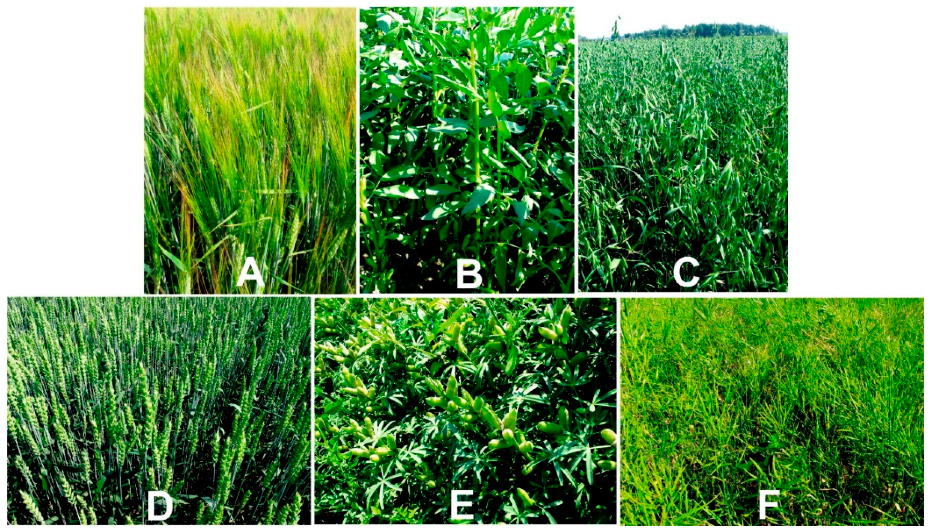
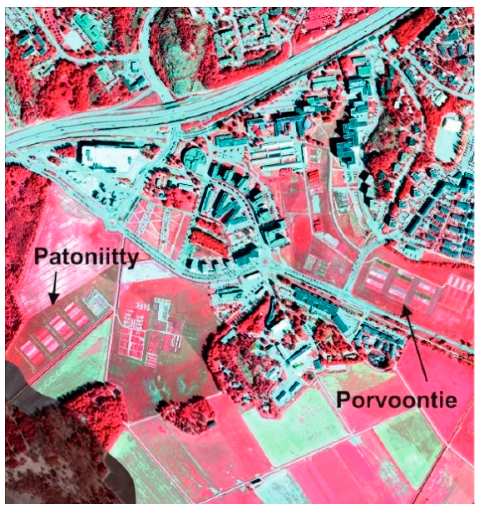
2.1. Field Plots

We used field data from 162 plots with six different crop species: oat (Avena sativa L.), turnip rape (Brassica rapa L. ssp. oleifera (DC.) Metzg.), barley (Hordeum vulgare L.), lupin (Lupinus angustifolius L.), wheat (Triticum aestivum L. emend Thell), and faba bean (Vicia faba L.) (Figure 1). The plots were located at the Patoniitty and Porvoontie agricultural experimental sites on the Viikki campus of the University of Helsinki, Finland (60.22° N, 25.02° E,

Table 1. Field plots measured in the study. Soil types: fertile luvic stagnosol and sandy clay loam (1), haplic gleysols and silty clay loam (2), sulfic cryaquepts (3), fertile luvic stagnosol and sandy medium clay loam (4) (WRB, 2007).

Species	Cultivars	No. of Plots	Soil Type
Oat	‘Ivory’, ‘Mirella’	4	3
Turnip rape	‘Apollo’	4	3
Barley	‘Streif’, ‘Chill’, ‘Fairytale’	10	3, 4
Lupin	‘HaagsBlaue’	4	3
Wheat	‘Amaretto’	99	1, 2, 3
Faba bean	‘Kontu’	40	1, 3
Total		162

, Figure 2). The plots varied in soil type, planting density and fertilization (Table 1).

We applied the species-specific leaf tilt angle distributions determined at the same experimental site by Zou et al. [11]. They measured the leaf tilt angle, defined as the angle between the leaf surface normal and the zenith, from leveled photographs taken approximately 1 m from the edge of the plots growing the crops. Leaves orthogonal to the camera viewing direction (i.e., with their normals inside the image plane) appeared in the photos as narrow lines. Zou et al. [11] determined the directions of these leaves (lines in photographs), thus quantifying their tilt angle distribution. Assuming that leaves were distributed uniformly in the azimuth direction, the tilt angle distribution was taken as representative of the whole canopy and the species in general. Finally, the leaf angle distribution was used to calculate leaf mean tilt angle (MTA).

We used the leaf chlorophyll a and b content (Cab) determined with a SPAD meter (SPAD-502, Minolta, Japan) on 19–22 July 2011 and reported by Zou et al. [13]. After a single leaf was inserted into the SPAD meter, the instrument determined its transmittance of red light quantified as a ‘SPAD value’. Zou et al. [13] converted these SPAD measurements to absolute chlorophyll content using a general relationship available in the literature [28]

$$\mathrm{Cab}(\mathsf{\mu }\mathrm{g}{\mathrm{cm}}^{-2})=0.0893({10}^{{\mathrm{SPAD}}^{0.265}}).$$

(1)

Altogether, 15−30 SPAD readings were converted (Equation (1)) and averaged for each plot [13].

The leaf area index data reported by Zou et al. [11] were applied in this study. Zou et al. [11] used measurements with a SunScan SSI ceptometer bar (Delta-T Devices, Cambridge, UK) on 20–21 July 2011 from the study plots. The ceptometer bar determined the canopy-penetrated photosynthetically active radiation under a clear sky using 64 miniature sensors. Within the instrument hardware, the readings were averaged and, using data from a separate top-of-canopy sensor, converted to the canopy transmittance of the direct solar beam. Zou et al. [11] used the standard method for converting canopy transmittance to LAI (based on the Beer–Lambert law of radiation extinction) with extinction coefficients determined from the leaf angle measurements described above. The mean values of LAI, MTA, and Cab for the plots used in this study are presented in Table 1, and further details have been reported by Zou and Mõttus [12].

We used the soil spectral reflectance measurements by Zou and Mõttus [12]. They determined the mean soil spectral reflectance from harvested plots using a handheld Analytical Spectral Devices spectrometer (ASD Inc., Boulder, CO, USA) and a white Spectralon reflectance panel under cloudless skies on 7 October 2011. Zou and Mõttus [12] corrected the measured reflectance for differences in the solar angle between the measurement times in July and October.

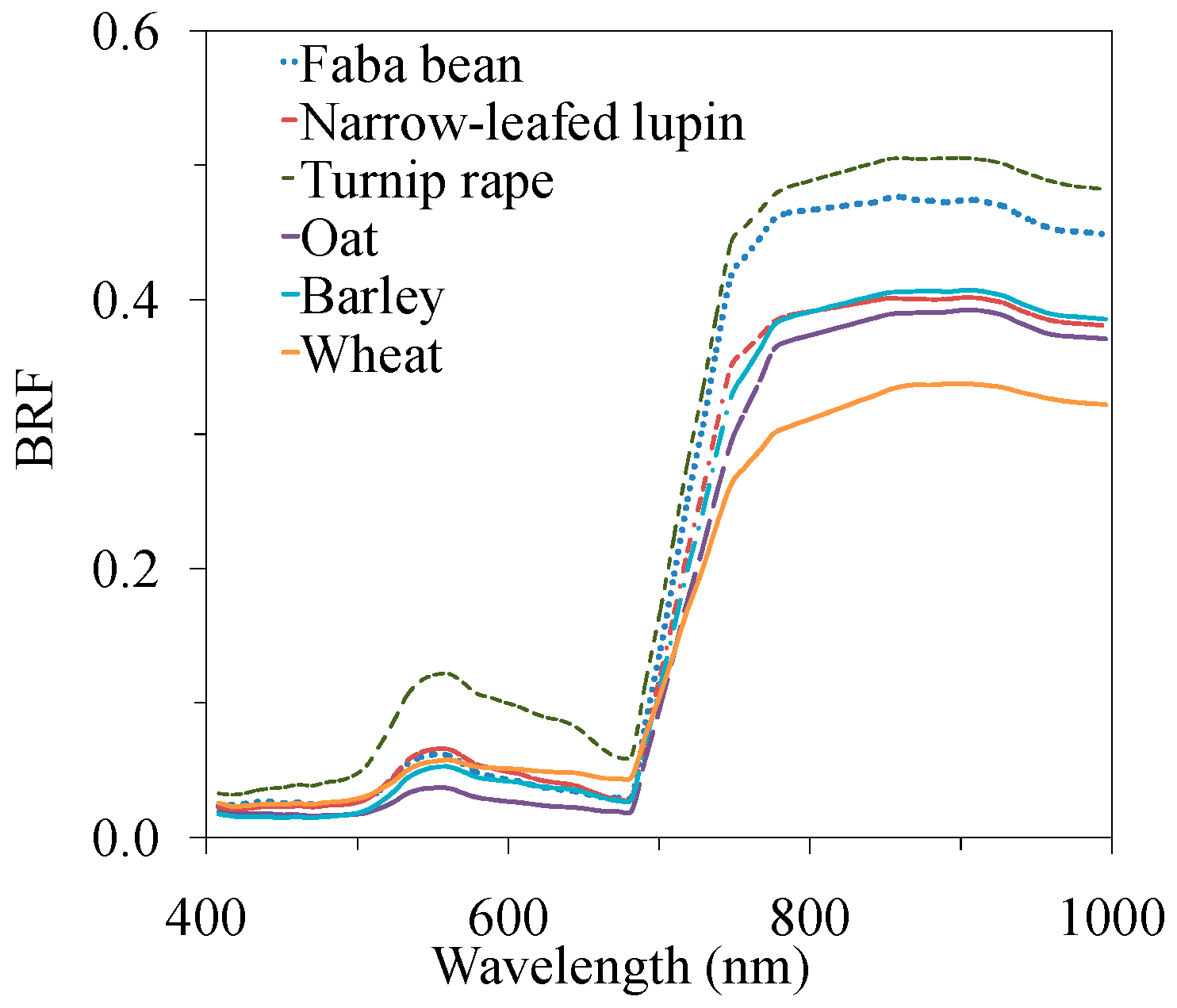
2.2. Remote Sensing Data

Airborne imaging spectroscopy data were acquired on 25 July 2011 using an AISA Eagle II push broom scanner (Spectral Imaging Ltd., Oulu, Finland) with an instantaneous field of view of 0.037° and a field of view of 37.7° [29]. The sensor produced data in 64 spectral channels with a full width at half maximum of 8.0–10.5 nm in the spectral range of 400–1000 nm. Data collection was performed from a height of 600 m between 09:36 a.m. and 10:00 a.m. local time, producing a spatial resolution of 0.4 m. The average solar zenith angle was 49.4° and the flight line direction was set to match the solar azimuth to minimize the influence of scattering anisotropy [30]. The spectral imagery was radiometrically calibrated and converted to top-of-canopy hemispherical-directional reflectance factors, as described by Zou et al. [11]. The spectral reflectance factors for each field plot were extracted from the imagery.

2.3. Model Simulations

Simulated canopy reflectance data were generated with the PROSAIL model [24], composed of the PROSPECT-5 [31,32] leaf optical model and the SAILH [33] canopy reflectance model. PROSPECT-5 simulates the hemispherical reflectance and leaf level transmittance by using Cab, the leaf carotenoid content, leaf dry matter content, leaf water content, leaf brown pigment content, and the leaf mesophyll structure parameter. SAILH additionally requires LAI, MTA, the solar zenith angle, sensor viewing angle, azimuth angle, the fraction of diffuse solar illumination, soil reflectance, and the hot-spot size parameter. We ran PROSAIL 100,000 times with input values drawn from the uniform distributions given by values of field measurements and the literature. Based on field measurements, we varied Cab between 25 and 100 µg cm⁻², LAI between 1 and 5, MTA between 15° and 70°, and the leaf water content between 0.001 and 0.020 cm. The leaf mesophyll structure parameter was fixed to 1.55, the average value of various crop species [34], and the leaf dry matter content to 0.005 g cm⁻², a value suitable for the six studied species [35,36,37,38]. The leaf carotenoid content was linked to Cab with the ratio 1:5 based on LOPEX93 data [39]. The brown pigment content was set to 0, assuming that the leaves were green during the measurement. The fraction of diffuse radiation was calculated with the 6S atmosphere radiative transfer model [40] using the input data derived from the image itself and the nearby sun photometer measurements. The hot-spot size parameter had a negligible effect on the simulation due to the observation geometry (sufficiently far from backscatter, or the hot spot) and was set to a reasonable value for a vegetation canopy (0.01). The view and illumination geometry parameters in the model were set to coincide with airborne measurement conditions (solar zenith angle 49.4°, sensor zenith angle 9°, and azimuth angle 90°). The soil reflectance was taken from measurements. A detailed description of the PROSAIL inputs is given by Zou and Mõttus [12]. The PROSAIL spectral resolution was 1 nm, and it was resampled to correspond to the wavelengths measured by AISA using a Gaussian spectral response function.

2.4. Vegetation Indices

Eight LAI-sensitive narrowband VIs (

Table 2. Narrow-band vegetation indices used in the study.

Vegetation Index	Equation	Central Wavelength Used in This Study	Reference
BNDVI	$\left({\mathrm{R}}_{800}-{\mathrm{R}}_{450}\right)/\left({\mathrm{R}}_{800}+{\mathrm{R}}_{450}\right)$	${\mathrm{R}}_{805}$, ${\mathrm{R}}_{452}$	[21]
GARI	${\mathrm{R}}_{800}/{\mathrm{R}}_{530}-1$	${\mathrm{R}}_{805}$, ${\mathrm{R}}_{533}$	[20]
GNDVI	$\left({\mathrm{R}}_{800}-{\mathrm{R}}_{530}\right)/\left({\mathrm{R}}_{800}+{\mathrm{R}}_{530}\right)$	${\mathrm{R}}_{805}$, ${\mathrm{R}}_{533}$	[22]
MSAVI	$0.5\left[2{\mathrm{R}}_{800}+1-\sqrt{{\left(2{\mathrm{R}}_{800}+1\right)}^2-8\left({\mathrm{R}}_{800}-{\mathrm{R}}_{680}\right)}\right]$	${\mathrm{R}}_{805}$, ${\mathrm{R}}_{682}$	[18]
MSR705	$\left({\mathrm{R}}_{750}/{\mathrm{R}}_{705}-1\right)/\sqrt{{\mathrm{R}}_{750}/{\mathrm{R}}_{705}+1}$	${\mathrm{R}}_{748}$, ${\mathrm{R}}_{701}$	[3]
NDVI	(${\mathrm{R}}_{800}-{\mathrm{R}}_{680})/\left({\mathrm{R}}_{800}+{\mathrm{R}}_{680}\right)$	${\mathrm{R}}_{805}$, ${\mathrm{R}}_{682}$	[16]
SAVI	$\left({\mathrm{R}}_{800}-{\mathrm{R}}_{680}\right)\left(1+0.5\right)/\left({\mathrm{R}}_{800}+{\mathrm{R}}_{680}+0.5\right)$	${\mathrm{R}}_{805}$, ${\mathrm{R}}_{682}$	[17]
SR	${\mathrm{R}}_{800}/{\mathrm{R}}_{680}$	${\mathrm{R}}_{805}$, ${\mathrm{R}}_{682}$	[19]

) were calculated from the spectral reflectance data collected with the airborne sensor and the simulated dataset. The indices were calculated using AISA bands and model-simulated AISA bands that were closest to the original wavelengths.

2.5. Statistical Methods and Data Analysis

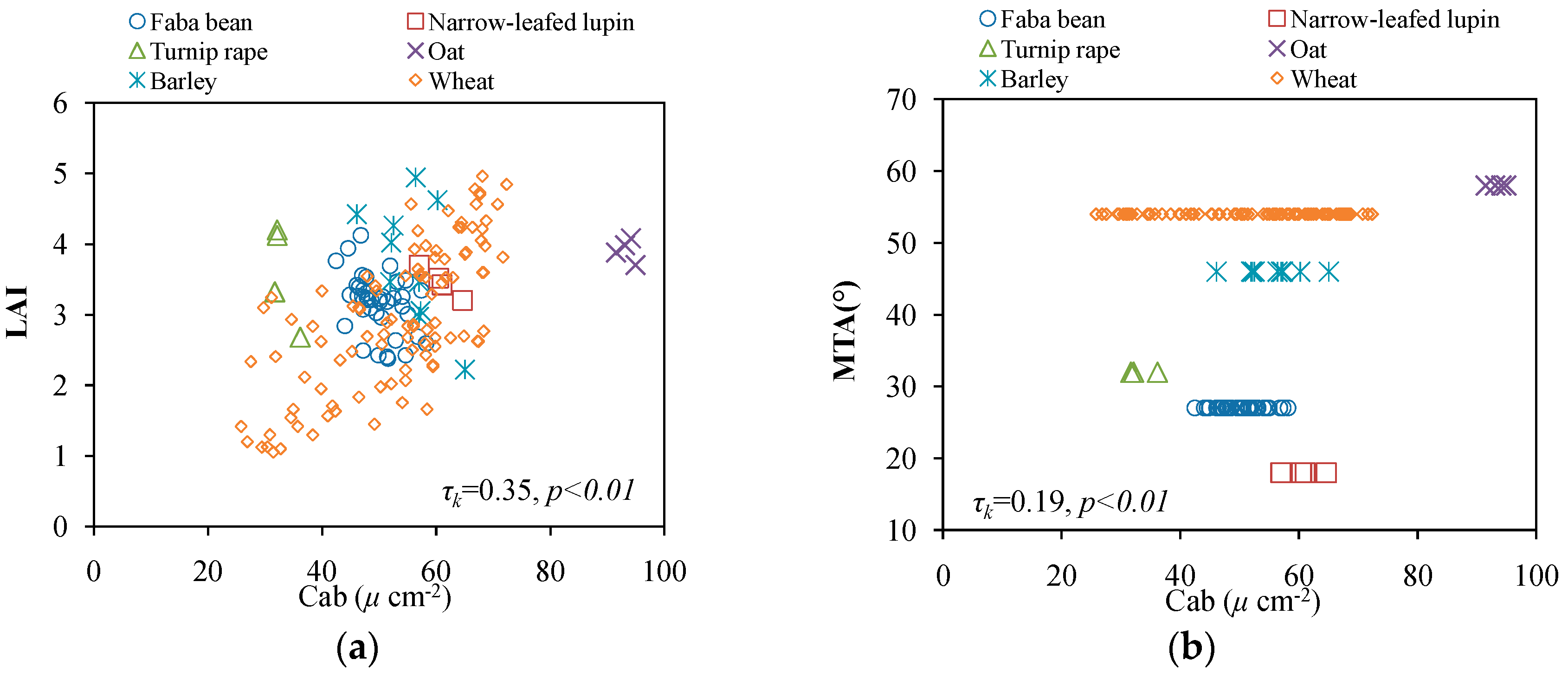
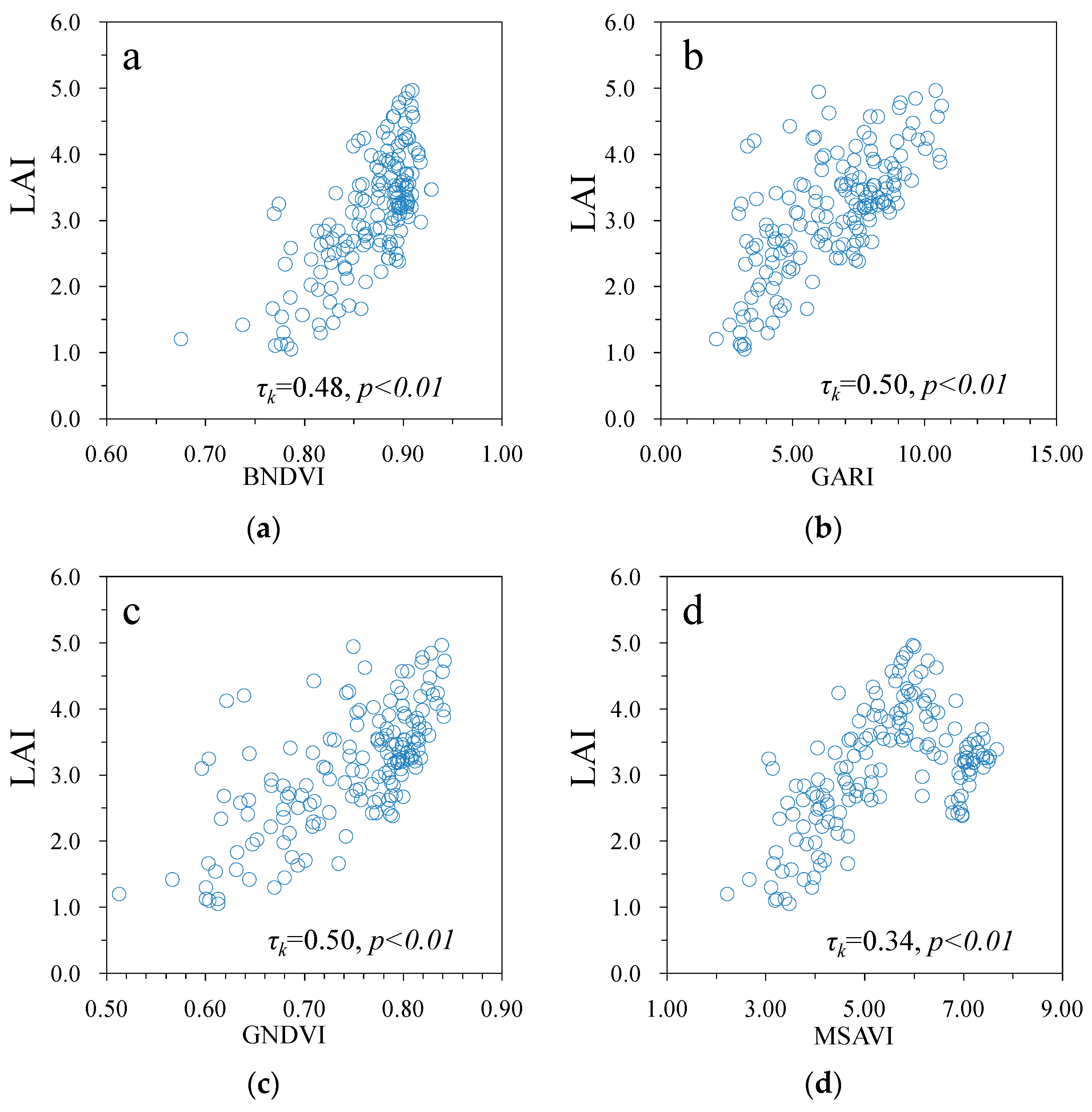
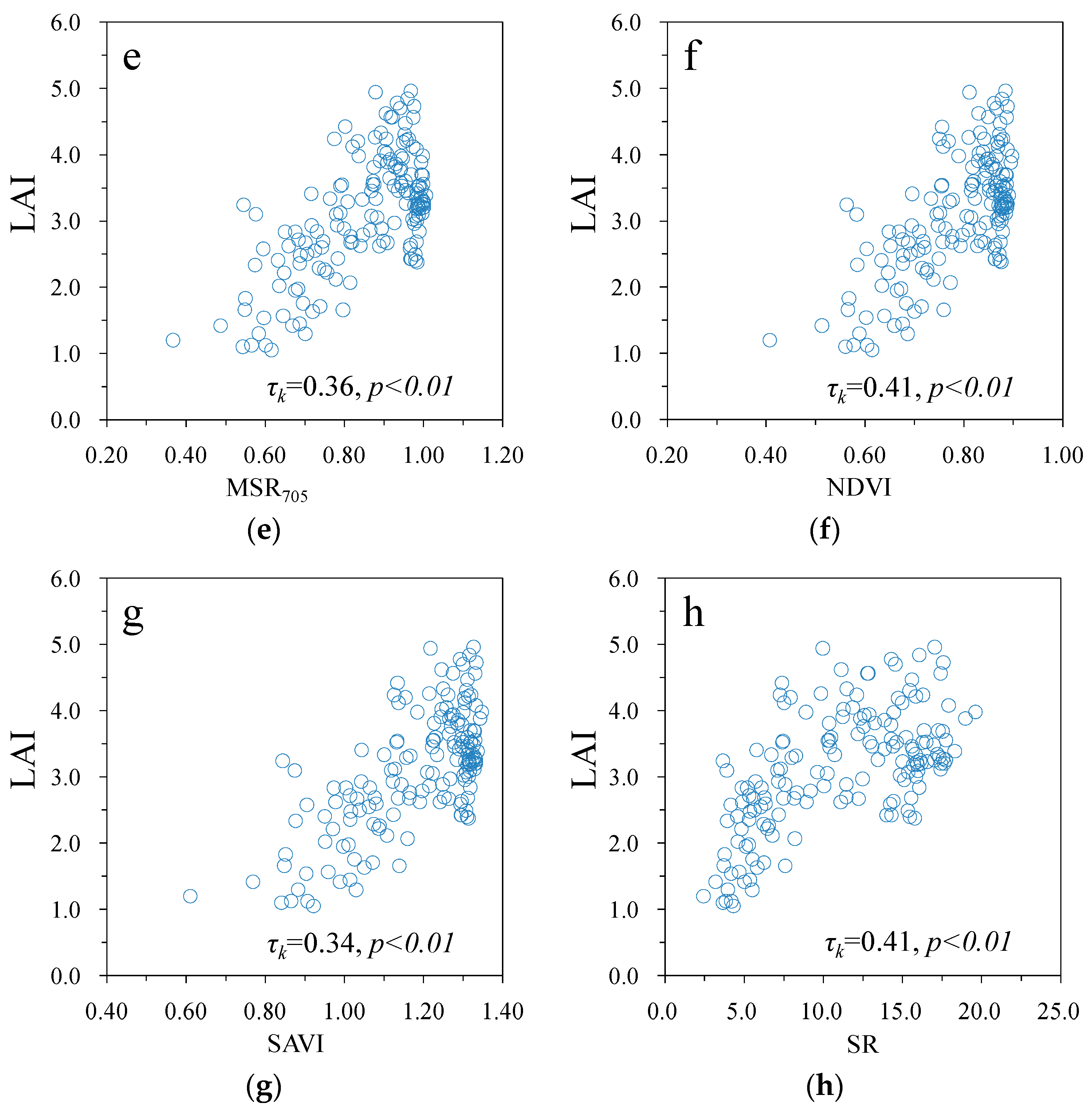
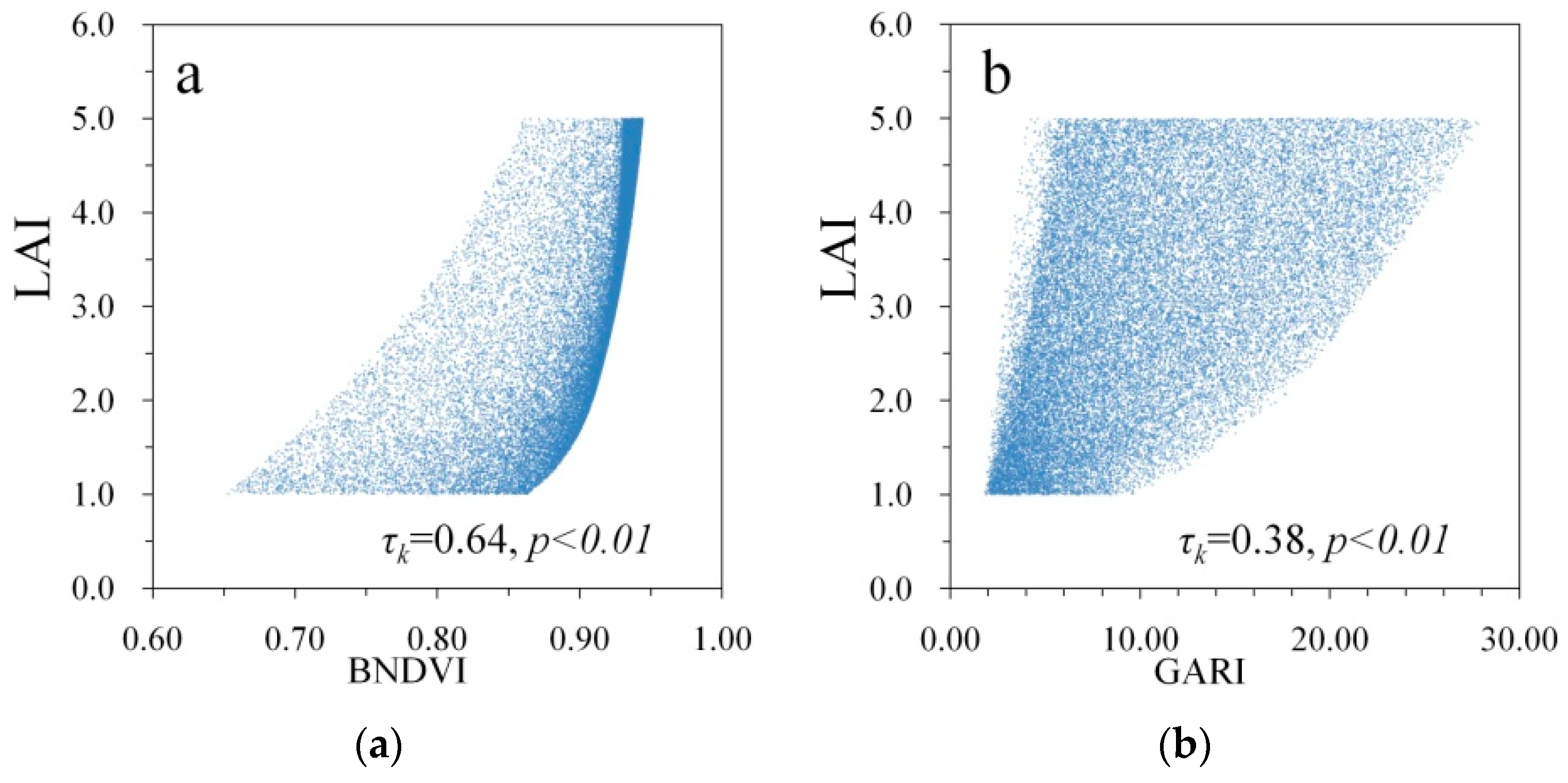
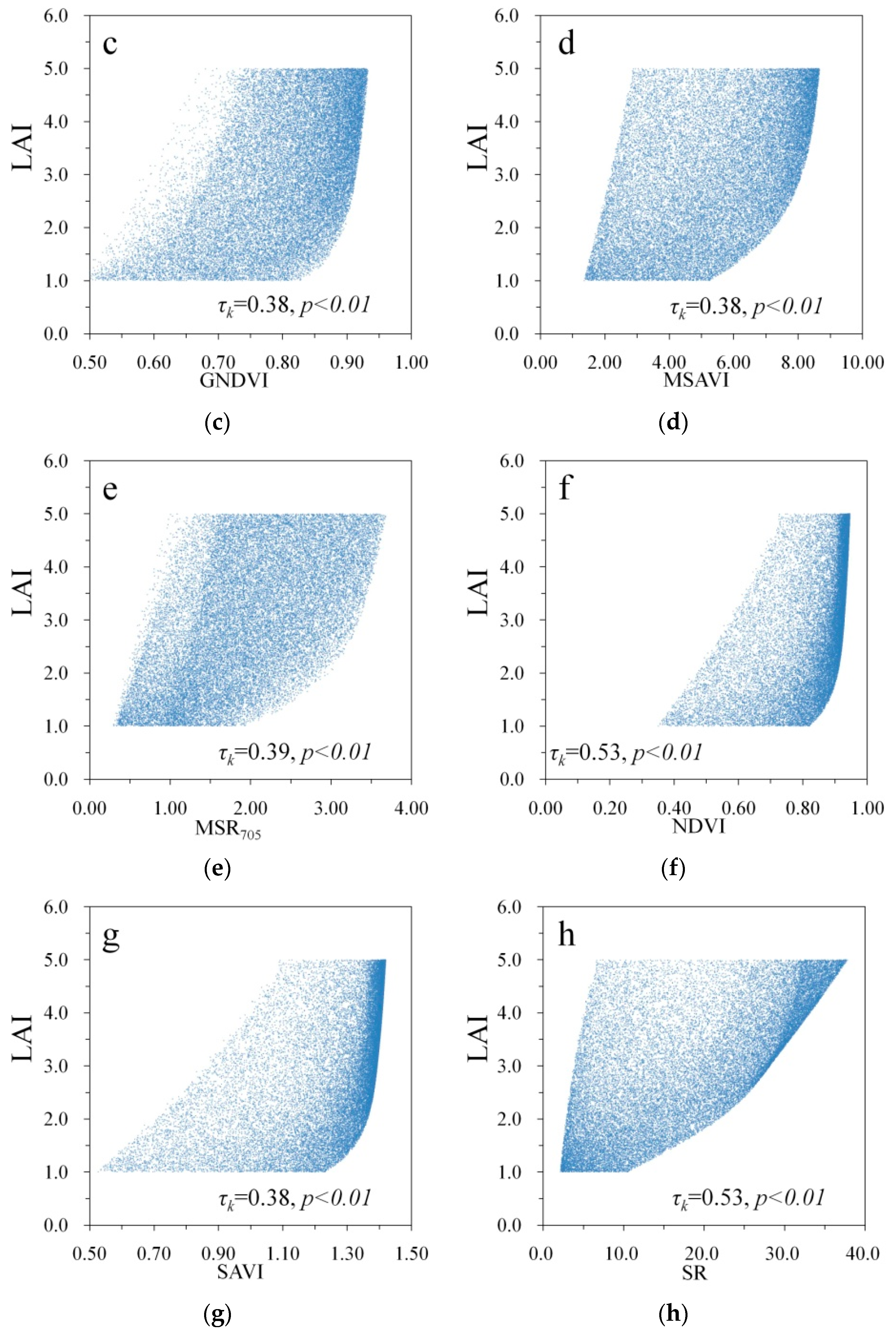
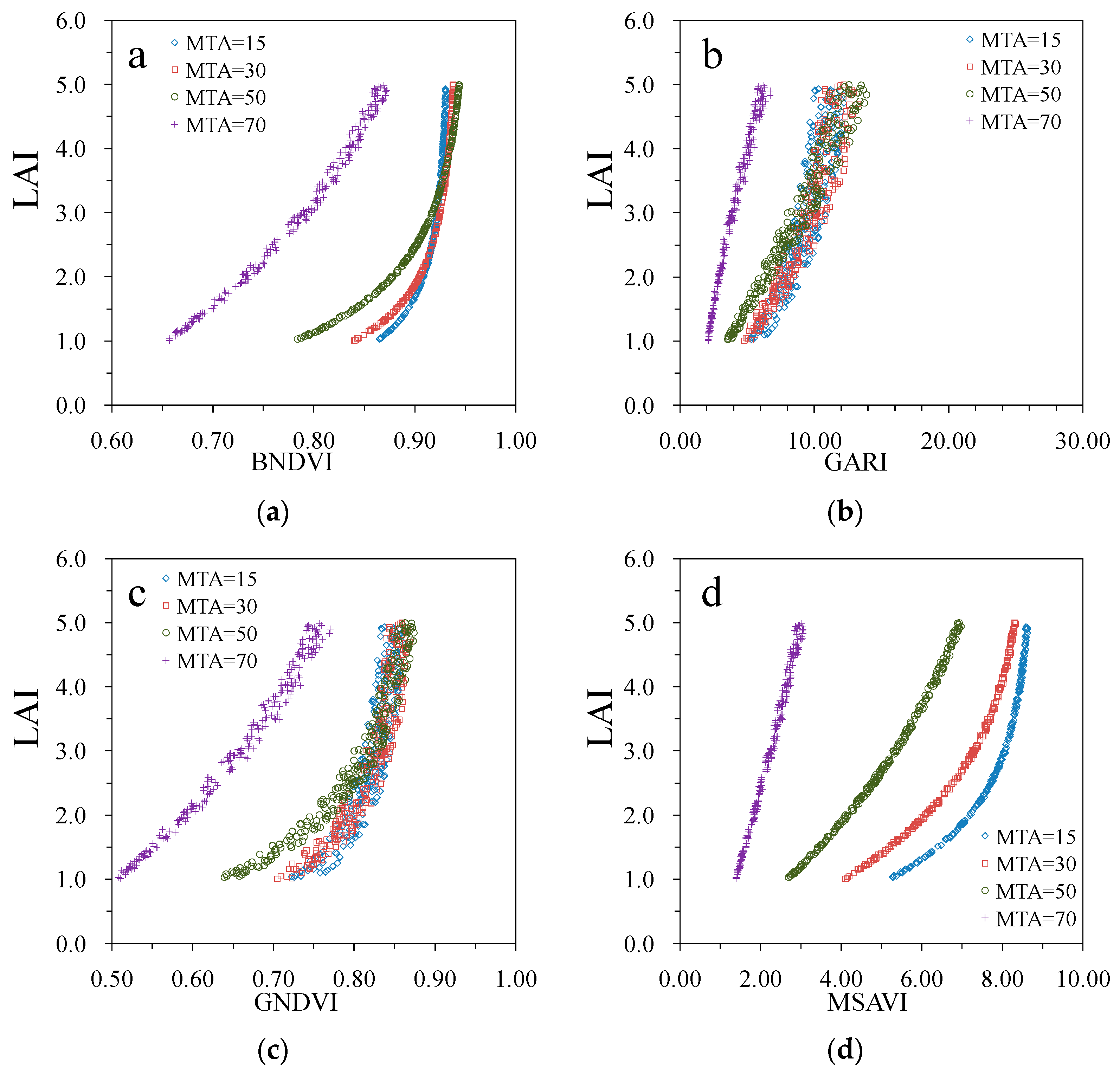
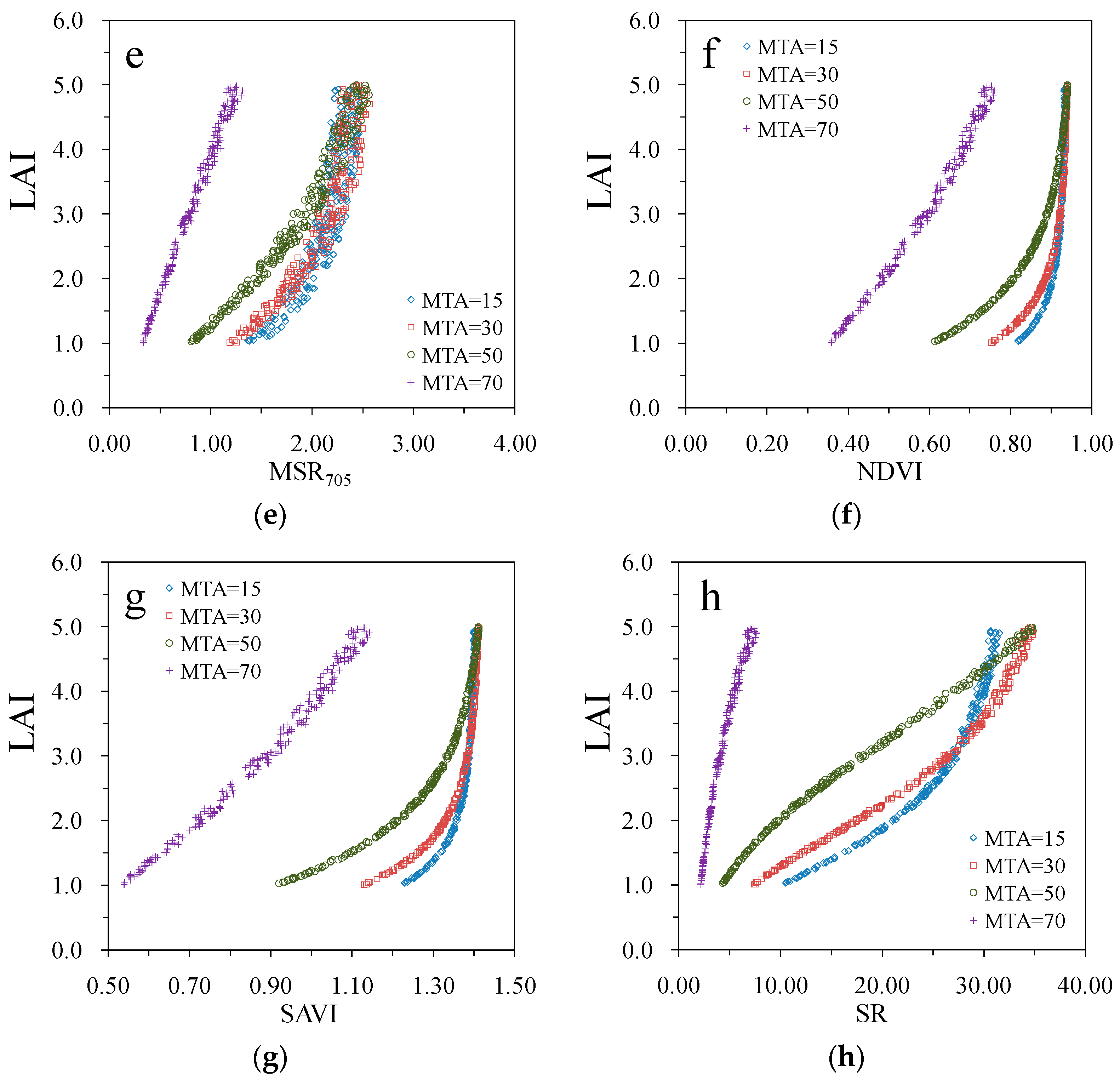
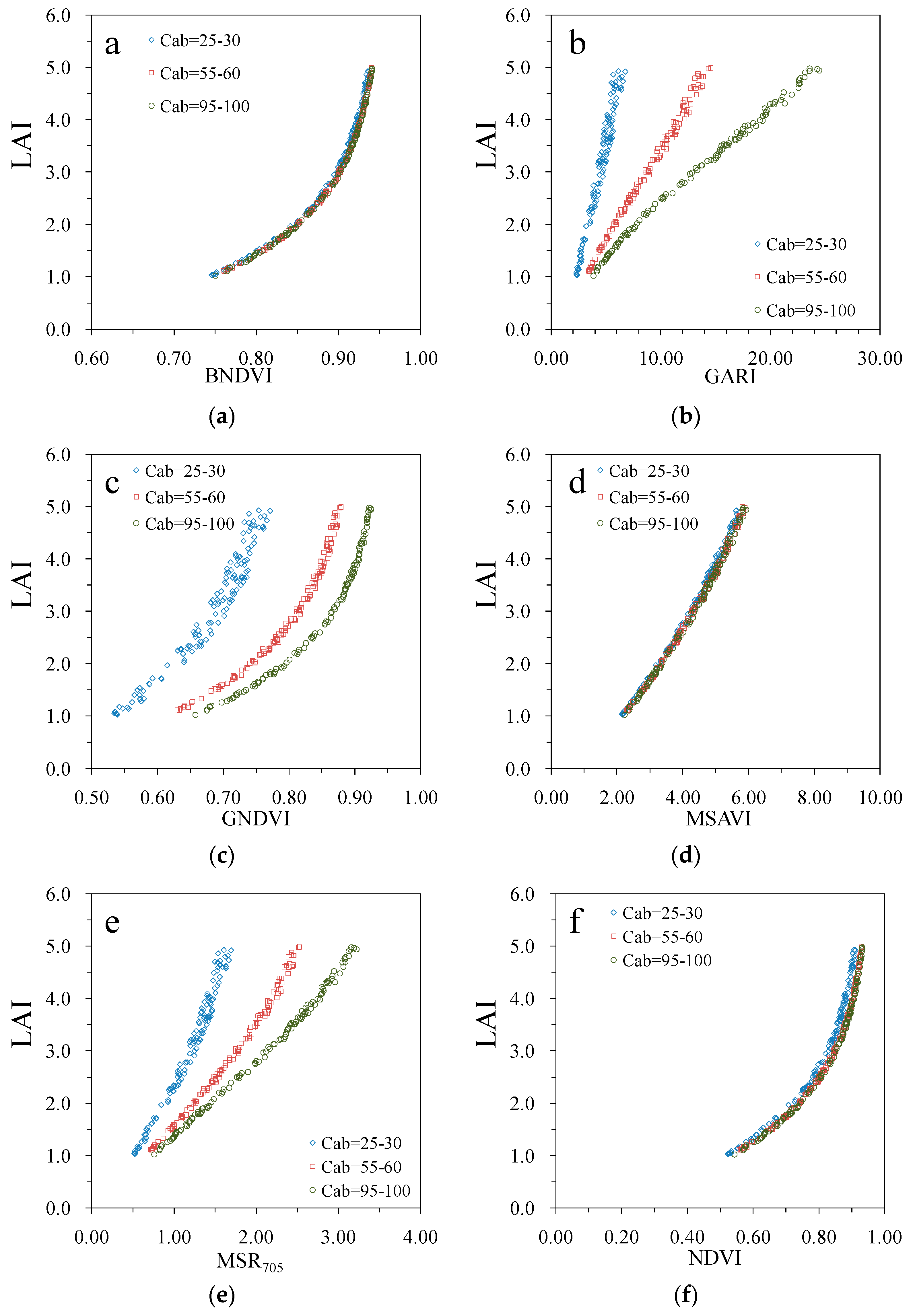
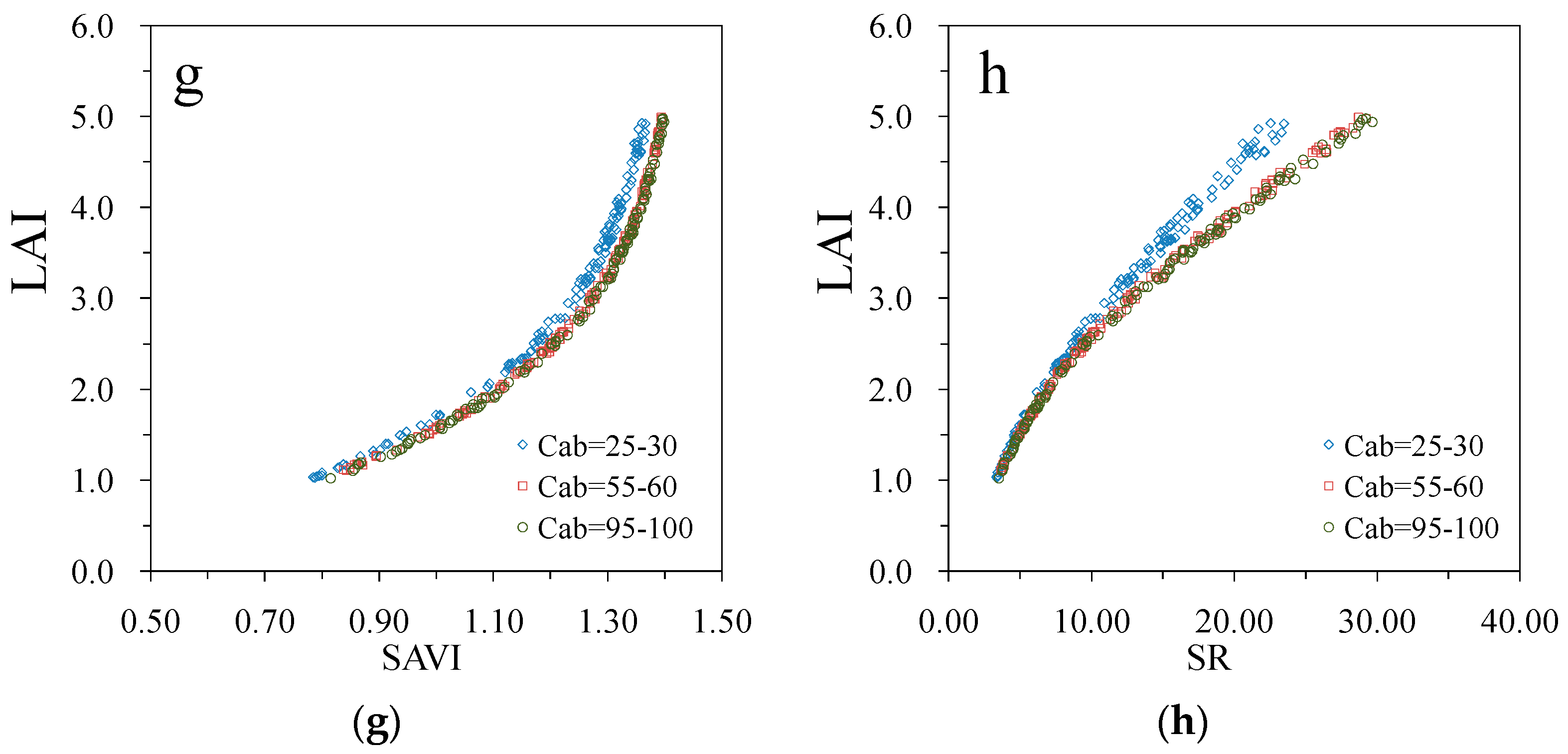
First, we examined the internal correlations within the field-measured crop parameter data to decide upon the potential limitations of the analyses. Next, we calculated the Kendall’s rank correlation coefficient (τ_k) between LAI and the selected VIs from both simulated and field-measured data. Kendall’s τ_k is a non-parametric measure of the strength of a monotonic relationship between paired data. The value of τ_k lies between −1 and 1, with τ_k = −1 indicating a perfect negative correlation between the paired data, τ_k = 0 the lack of a relationship and τ_k = 1 a perfect positive correlation. We chose τ_k instead of the more standard Pearson’s correlation coefficient R (and the related coefficient of determination R²) because the field data did not satisfy the assumption of normality. Neither did we have to assume a linear relationship between the vegetation parameters and VIs. Despite similar ranges, the numerical value of τ_k for a relationship between any two variables is generally different from R.

To determine how MTA affects the performance of the indices in estimating LAI, we fixed Cab in the simulated data by extracting simulations with Cab between 45–50 µg cm⁻². Next, we divided the simulations into groups based on MTA (15°, 30°, 50°, and 70°) and plotted the VIs calculated from the data against LAI. Similarly, we fixed MTA at 57° and varied Cab between three levels (25–30, 55–60, and 95–100 µg cm⁻²) to estimate the effect of Cab on the VI–LAI relationship. Due to the imbalance in the measured actual species-specific leaf angles caused by an uneven distribution of samples between species, we could not analyze the sensitivity of the VI–LAI relationship to MTA in the field-measured dataset.

3. Results

The average reflectances of all measured species were typical vegetation reflectance spectra, but still dissimilar when examined in detail (Figure 3). For example, turnip rape had the largest reflectance across the measured spectral range. Wheat had the lowest reflectance in NIR, but the second-highest in red and average in green. The field-measured mean LAI for each species was between 3 and 4 (

Table 3. Key characteristics of field plots measured in the study. LAI: leaf area index, MTA: mean tilt angle, Cab: chlorophyll a and b content.

Species	Average LAI	MTA (°)	Average Cab (µg cm−2)
Oat	3.91	58	93
Turnip rape	3.58	32	33
Barley	3.74	46	56
Lupin	3.46	18	61
Wheat	2.96	64	53
Faba bean	3.16	27	50

), while individual plot-level measurements varied between 1 and 5 (Figure 4a). Cab varied between 25 and 95 µg cm⁻² (Table 3, Figure 4a,b). Oat had the highest Cab (93 µg cm⁻²) and turnip rape the lowest value (32 µg cm⁻²). There was a significant (p < 0.01) relationship between the field-measured LAI and Cab, with τ_k = 0.35 (Figure 4a), and a weaker (τ_k = 0.19), yet still significant, correlation between the photographic MTA and Cab (Figure 4b).

All used VIs were correlated with LAI in both the field-measured and model-simulated data (

Table 4. Kendall’s rank correlation coefficient (τ_k) between vegetation indices and LAI for model simulations and field-measured data. All correlations were statistically significant (p < 0.01).

Vegetation Index	Model Simulation	Field Measurements
BNDVI	0.64	0.48
GARI	0.38	0.50
GNDVI	0.38	0.50
MSAVI	0.38	0.34
MSR705	0.39	0.36
NDVI	0.53	0.41
SAVI	0.38	0.34
SR	0.53	0.41

), with τ_k between 0.34 and 0.64. For the field-measured data (Figure 5), the rank correlation coefficients were all above 0.4, except for MSAVI, MSR₇₀₅, and SAVI (τ_k = 0.34–0.36), and with GARI and GNDVI performing best among the tested VIs (τ_k = 0.50). In model simulations (Figure 6), GARI and GNDVI produced the lowest τ_k of 0.38, with BNDVI being the most strongly correlated (τ_k = 0.64). All the relationships for both empirical analysis and model simulations were significant (p < 0.01).

The correlations between VIs and LAI were improved when MTA was fixed, with τ_k > 0.7 at all four MTA levels (

Table 5. Kendall’s rank correlation coefficient (τ_k) between vegetation indices and LAI in PROSAIL-simulated data for different MTA values at a fixed Cab (45–50 µg cm⁻²). All correlations were statistically significant (p < 0.01).

Vegetation Index	MTA = 15°	MTA = 30°	MTA = 50°	MTA = 70°
BNDVI	0.98	0.99	0.99	0.95
GARI	0.72	0.80	0.88	0.93
GNDVI	0.72	0.80	0.88	0.93
MSAVI	0.98	0.98	0.98	0.94
MSR705	0.73	0.83	0.91	0.94
NDVI	0.93	0.97	0.98	0.95
SAVI	0.93	0.97	0.98	0.95
SR	0.95	0.98	0.99	0.95

). The relationships between VIs and LAI were most notably affected at MTA > 60°; at a lower MTA, the effect of leaf angle was less evident (Figure 7), especially for BNDVI, GARI, GNDVI, NDVI, and MSR₇₀₅ at LAI > 3 (Figure 7a,f,g). The effect of MTA on the VI–LAI relationship increased as a function of decreasing LAI for BNDVI, GNDVI, MSR₇₀₅, NDVI, and SAVI; for the remaining indices, the trend was unclear. Across the whole studied LAI variation range, the VI–LAI relationships for MSAVI and SR were most strongly affected by MTA, as the point clouds corresponding to the distinct MTA levels are clearly separable in Figure 7d,h. On the other hand, SR was the least saturating VI with LAI, and the relationships were nearly linear for the whole LAI range at MTA 15–50° (Figure 7h).

The leaf chlorophyll content only weakly affected the relationship between BNDVI, MSAVI, NDVI, SAVI, and LAI (Figure 8a,d,f,g), as the point clouds corresponding to the different Cab values overlap in the figure. For the other indices (GARI, GNDVI, MSR₇₀₅, and, to a smaller extent, SR; Figure 8b,c,e,h), relationships with LAI were clearly affected by Cab, with the influence of Cab generally increasing as a function of LAI.

4. Discussion

The field data used in this analysis had some inherent natural limitations. For example, the leaf chlorophyll content (Cab) and green LAI are often closely related [41], which was also the case for the field data used in the study (Figure 4). As the application of nitrogen increases the chlorophyll content [42], the level of fertilization has an impact on the performance of LAI-sensitive VIs if these also depend on Cab. Furthermore, a similar indirect influence of Cab on the studied VIs is possible if the Cab values are dominated by between-species differences. In addition to natural correlations, the experimental design of the study was not fully driven by the objectives of this research. We used the field data available from numerous crop management experiments carried out in the area covered by airborne IS data. We accounted for the imbalanced nature of the field data as much as possible and used crop reflectance simulations of uniformly distributed input parameters for generalization.

Our results, both computer simulated and those retrieved from field data, are generally consistent with the numerous published findings, which state that the selected VIs can indeed be utilized for measuring LAI with remote sensing (e.g., [23]): τ_k was between 0.34 and 0.64 for all the selected VIs. However, the relationship was nonlinear [20,43], and some indices (e.g., NDVI) saturated at high LAI values [44].

In both field-measured and simulated data, correlation coefficients between VIs and LAI were low (τ_k was between 0.34 and 0.64), even though the selected indices were clearly sensitive to LAI. This is in agreement with other studies [26,45,46], which have found a wide range of coefficients of determination (0.05 < R² < 0.66) between VIs and LAI. It is known that differences between crop species affect the goodness of fit more than the vegetation indices used [47]. Evidently, the coefficients were affected by the large volume of simulated data and the range of species with different characteristics in the true data. Both datasets included sufficient structural and biochemical variation to blur the relationships between LAI and VIs. Estimating the LAI of heterogeneous vegetated areas (with subpixel heterogeneity) from remote sensing data is hence not as reliable as estimation of the LAI of homogeneous fields. This is demonstrated by Figure 7 and Table 5, where the correlations improved and correlation coefficients increased from the range of 0.38–0.64 to 0.72–0.93 when a structural parameter, MTA, was fixed. Other studies have also shown the relationship between VIs and LAI to vary across vegetation types (canopy architecture) and the correlations to improve when analyzing the relationship between VIs and LAI for each vegetation type separately [48,49]. The leaf angle distribution, and thus MTA, affects the spectral properties of a canopy [50] to a degree that confuses LAI estimation algorithms based on simple VIs [50].

Based on its performance in both field-measured and model-simulated data, the best index was BNDVI. It was only slightly sensitive to MTA, especially for low LAI values (Figure 7a), and insensitive to Cab (Figure 8a). Two indices (GARI, GNDVI) (τ_k = 0.50) performed slightly better than BNDVI (τ_k = 0.48) in the field study and were insensitive to MTA (Figure 7b,c). Unfortunately, both indices were sensitive to Cab (Figure 8b,c). For example, at a medium LAI (LAI = 3), when Cab increased from low levels (25–30 µg cm⁻²) to high levels (95–100 µg cm⁻²), the indices increase by approximately 50% of their whole range of variation (Figure 8b,c), and hence did not show a strong correlation with LAI in the model-simulated data (τ_k = 0.38). On the other hand, BNDVI (similarly to GNDVI) clearly saturated with LAI (Figure 7a,c), while GARI was more linear with LAI (Figure 7b). The slope of the GARI–LAI relationship, however, depended on Cab (Figure 8b). The slope varied from 0.94 to 0.19 when Cab increased from low (25–30 µg cm⁻²) to high levels (95–100 µg cm⁻²). SR displayed only slight saturation with LAI, regardless of MTA and the chlorophyll content. This index was largely insensitive to Cab (Figure 8h) and showed similar slopes (approximately 0.15) when plotted against LAI for MTA < 60°. Unfortunately, MTA created varying offsets in the LAI–SR relationship (Figure 7h). As a result, SR showed only an average performance, with τ_k = 0.41 and 0.53 in the field-measured and model-simulated datasets, respectively. Nevertheless, it could be the index of choice for mapping areas with limited variations in structure, e.g., covered by the same crop species. Indeed, together with MSAVI, SR was among the indices independent of Cab and producing the most linear relationships with LAI (Figure 8). For reasons unknown to us, MSAVI and SAVI were the worst performers with field-measured data (Table 4) and hence cannot be recommended based on this study.

LAI and Cab affect canopy reflectance in a similar manner [51] in visible and near-infrared spectral regions, explaining the better performance of VIs in LAI estimation under high Cab. Although the relationships between VIs and LAIs may be tight for a limited set of species under a controlled environment, MTA, as well as other structural parameters, causes scatter in these relationships at larger scales and thus reduces the LAI retrieval capacity of the VIs. This may make the design of a universal optimal spectral index for all crops and growth conditions impossible [52]. LAI can still be rapidly and reliably estimated using VIs in breeding projects with limited within-sample structural variation in which early vigor is of interest. LAI estimation can be used to select the populations with the greatest leaf area as the most vigorous ones, as early vigor gives an advantage over weeds [53,54]. VI-based LAI estimation could also be potentially used in optimizing crop production and the development of best crop management practices, such as the timing of application of water, fertilizers, and pesticides [55,56,57].

5. Conclusions

Based on empirical measurements and model simulations, the effects of the leaf angle and chlorophyll content on LAI-sensitive narrow-band indices were examined. Kendall’s correlation coefficients between LAI and the vegetation indices were between 0.34 and 0.64 for all the tested indices. The accuracy of the indices in estimating LAI was restricted by the variation in MTA and Cab. The relationship was stronger within specific canopy architectures (defined by a constant MTA), making it difficult to estimate LAI using VIs for areas covered by different vegetation types. Of the studied indices, we found BNDVI to be the least affected by the leaf tilt angle and chlorophyll content, and thus the most suitable one for retrieving LAI using remote sensing (τ_k = 0.64 for empirical data). Nevertheless, the performance of all studied VIs in LAI estimation, including BNDVI, was affected by the leaf tilt angle, especially at LAI < 3. Most of the studied indices were suitable for monitoring the LAI of crops with a constant leaf angle distribution (Kendall’s tau τ_k > 0.7 in the simulated dataset), with SR outperforming others in linearity and applicability to both measured and simulated data. In the future, more crop species with different leaf angle distributions, leaf pigment contents, contrasting canopy architectures, and different growth stages should be used to empirically validate the effects of leaf angle and Cab on LAI-sensitive indices, so that the results can be applied to a wider geographic region.

References

1. Watson, D.J. Comparative physiological studies on the growth of field crops: I, Variation in net assimilation rate and leaf area between species and varieties, and within and between years. Ann. Bot. 1947, 11, 41–76. [Google Scholar] [CrossRef]
2. Daughtry, C.S.T.; Gallo, K.P.; Goward, S.N.; Prince, S.D.; Kustas, W.D. Spectral estimates of absorbed radiation and phytomass production in corn and soybean canopies. Remote Sens. Environ. 1992, 39, 141–152. [Google Scholar] [CrossRef]
3. Chen, J.M.; Black, T.A. Defining leaf area index for non-flat leaves. Plant Cell Environ. 1992, 15, 421–429. [Google Scholar] [CrossRef]
4. Ross, J. The Radiation Regime and Architecture of Plant Stands; Dr. W. Junk: The Hague, The Netherlands, 1981; p. 391. [Google Scholar]
5. Smith, W.K.; Bell, D.T.; Shepherd, K.A. Associations between leaf structure, orientation, and sunlight exposure in five western Australian communities. Am. J. Bot. 1998, 85, 56–63. [Google Scholar] [CrossRef] [PubMed]
6. Pellikka, P. Application of vertical wide–angle photography and airborne video data for phenological studies of beech forests in the German Alps. Int. J. Remote Sens. 2001, 22, 2675–2700. [Google Scholar] [CrossRef]
7. Haboudane, D.; Miller, J.R.; Pattey, E.; Zarco-Tejada, P.J.; Strachan, I. Hyperspectral vegetation indices and novel algorithms for predicting green LAI of crop canopies: Modeling and validation in the context of application to precision agriculture. Remote Sens. Environ. 2004, 90, 337–352. [Google Scholar] [CrossRef]
8. Clevers, J.G.P.W.; Jongschaap, R. Imaging Spectrometry for Agricultural Applications. In Imaging Spectrometry; Van de Meer, F.D., De Jong, S.M., Eds.; Kluwer Academic Publishers: Dordrecht, The Netherlands, 2001; pp. 157–199. [Google Scholar]
9. Curran, P.J.; Dungan, J.L.; Macler, B.A.; Plummer, S.E. The effect of a red leaf pigment on the relationship between red edge and chlorophyll concentration. Remote Sens. Environ. 1991, 39, 69–76. [Google Scholar] [CrossRef]
10. Wu, C.; Han, X.; Niu, Z.; Dong, J. An evaluation of EO-1 hyperspectral Hyperion data for chlorophyll content and leaf area index estimation. Int. J. Remote Sens. 2010, 31, 1079–1086. [Google Scholar] [CrossRef]
11. Zou, X.; Mõttus, M.; Tammeorg, P.; Torres, C.L.; Takala, T.; Pisek, J.; Mäkelä, P.; Stoddard, F.L.; Pellikka, P. Photographic measurement of leaf angles in field crops. Agric. For. Meteorol. 2014, 184, 137–146. [Google Scholar] [CrossRef]
12. Zou, X.; Mõttus, M. Retrieving crop leaf tilt angle from imaging spectroscopy data. Agric. For. Meteorol. 2015, 205, 73–82. [Google Scholar] [CrossRef]
13. Zou, X.; Hernández-Clemente, R.; Tammeorg, P.; Lizarazo Torres, C.; Stoddard, F.L.; Mäkelä, P.; Pellikka, P.; Mõttus, M. Retrieval of leaf chlorophyll content in field crops using narrow-band indices: Effects of leaf area index and leaf mean tilt angle. Int. J. Remote Sens. 2015, 36, 6031–6055. [Google Scholar] [CrossRef]
14. Zou, X.; Mõttus, M. Sensitivity of Common Vegetation Indices to the Canopy Structure of Field Crops. Remote Sens. 2017, 9, 994. [Google Scholar] [CrossRef]
15. Huete, A.; Didan, K.; Miura, T.; Rodriguez, E.P.; Gao, X.; Ferreira, L.G. Overview of the radiometric and biophysical performance of the MODIS vegetation indices. Remote Sens. Environ. 2002, 83, 195–213. [Google Scholar] [CrossRef]
16. Rouse, J.W.; Haas, R.H.; Schell, J.A.; Deering, D.W.; Harlan, J.C. Monitoring the Vernal Advancement and Retrogradation (Greenwave Effect) of Natural Vegetation. In NASA/GSFC Type III Final Report; NASA/GSFC: Greenbelt, MD, USA, 1974; p. 371. [Google Scholar]
17. Huete, A.R. A soil-adjusted vegetation index (SAVI). Remote Sens. Environ. 1988, 25, 295–309. [Google Scholar] [CrossRef]
18. Qi, J.; Chehbouni, A.; Huete, A.R.; Kerr, Y.H.; Sorooshian, S. A modified soil adjusted vegetation index. Remote Sens. Environ. 1994, 48, 119–126. [Google Scholar] [CrossRef]
19. Jordan, C.F. Derivation of leaf area index from quality of light on the forest floor. Ecology. 1969, 50, 663–666. [Google Scholar] [CrossRef]
20. Gitelson, A.A. Remote estimation of leaf area index and green leaf biomass in maize canopies. Geophys. Res. Lett. 2003, 30, 1248. [Google Scholar] [CrossRef]
21. Wang, F.M.; Huang, J.F.; Tang, Y.L.; Wang, X.Z. New vegetation index and its application in estimating leaf area index of rice. Rice Sci. 2007, 14, 195–203. [Google Scholar] [CrossRef]
22. Gitelson, A.A.; Kaufman, Y.J.; Merzlyak, M.N. Use of a green channel in remote sensing of global vegetation from EOS-MODIS. Remote Sens. Environ. 1996, 58, 289–298. [Google Scholar] [CrossRef]
23. Chen, J.M. Evaluation of vegetation indices and a modified ratio for boreal applications. Can. J. Remote Sens. 1996, 22, 229–242. [Google Scholar] [CrossRef]
24. Campbell, G.S.; Norman, J.M. An Introduction to Environmental Biophysics; Springer: New York, NY, USA, 1998. [Google Scholar]
25. Weiss, M.; Baret, F.; Smith, G.J.; Jonckheere, I.; Coppin, P. Review of methods for in situ leaf area index (LAI) determination. Part II. Estimation of LAI, errors and sampling. Agric. For. Meteorol. 2004, 121, 37–53. [Google Scholar] [CrossRef]
26. Daughtry, C.S.T.; Walthall, C.L.; Kim, M.S.; De Colstoun, E.B.; McMurtrey, J.E., III. Estimating corn leaf chlorophyll concentration from leaf and canopy reflectance. Remote Sens. Environ. 2000, 74, 229–239. [Google Scholar] [CrossRef]
27. Haboudane, D.; Tremblay, N.; Miller, J.R.; Vigneault, P. Remote estimation of crop chlorophyll content using spectral indices derived from hyperspectral data. IEEE Trans. Geosci. Remote Sens. 2008, 46, 423–437. [Google Scholar] [CrossRef]
28. Vohland, M.; Mader, S.; Dorigo, W. Applying different inversion techniques to retrieve stand variables of summer barley with PROSPECT + SAIL. Int. J. Appl. Earth Obs. Geoinf. 2010, 12, 71–80. [Google Scholar] [CrossRef]
29. Piiroinen, R.; Heiskanen, J.; Mõttus, M.; Pellikka, P. Classification of crops across heterogeneous agricultural landscape in Kenya using AisaEAGLE imaging spectroscopy data. Int. J. Appl. Earth Obs. Geoinf. 2015, 39, 1–8. [Google Scholar] [CrossRef]
30. Pellikka, P.; King, D.J.; Leblanc, S.G. Quantification and reduction of bidirectional effects in deciduous forest in aerial CIR imagery using two reference land surface types. Remote Sens. Rev. 2000, 19, 259–291. [Google Scholar] [CrossRef]
31. Jacquemoud, S.; Verhoef, W.; Baret, F.; Bacour, C.; Zarco-Tejada, P.; Asner, G.P.; François, C.; Ustin, S.L. PROSPECT + SAIL models: A review of use for vegetation characterization. Remote Sens. Environ. 2009, 113, S56–S66. [Google Scholar] [CrossRef]
32. Feret, J.B.; François, C.; Asner, G.P.; Gitelson, A.A.; Martin, R.E.; Bidel, L.P.R.; Ustin, S.L.; Le Maire, G.; Jacquemoud, S. PROSPECT-4 and 5: Advances in the leaf optical properties model separating photosynthetic pigments. Remote Sens. Environ. 2008, 112, 3030–3043. [Google Scholar] [CrossRef]
33. Verhoef, W. Light scattering by leaf layers with application to canopy reflectance modeling: The SAIL model. Remote Sens. Environ. 1984, 16, 125–141. [Google Scholar] [CrossRef] [Green Version]
34. Haboudane, D.; Miller, J.R.; Tremblay, N.; Zarco-Tejada, P.J.; Dextraze, L. Integrated narrow-band vegetation indices for prediction of crop chlorophyll content for application to precision agriculture. Remote Sens. Environ. 2002, 81, 416–426. [Google Scholar] [CrossRef]
35. Mäkelä, P.; Kleemola, J.; Jokinen, K.; Mantila, J.; Pehu, E.; Peltonen-Sainio, P. Growth response of pea and summer turnip rape to foliar application of glycinebetaine. Acta Agric. Scand. Sect. B Soil Plant. Sci. 1997, 47, 168–175. [Google Scholar] [CrossRef]
36. Dennett, M.D.; Ishag, K.H.M. Use of the Expolinear Growth Model to Analyze the Growth of Faba Bean, Peas and Lentils at Three Densities: Predictive Use of the Model. Ann. Bot. 1998, 82, 507–512. [Google Scholar] [CrossRef]
37. Pinheiro, C.; Rodrigues, A.P.; De Carvalho, I.S.; Chaves, M.M.; Ricardo, C.P. Sugar metabolism in developing lupin seeds is affected by a short-term water deficit. J. Exp. Bot. 2005, 56, 2705–2712. [Google Scholar] [CrossRef] [PubMed] [Green Version]
38. Vile, D.; Garnier, E.; Shipley, B.; Laurent, G.; Navas, M.L.; Roumet, C.; Lavorel, S.; Diaz, S.; Hodgson, J.G.; Lloret, F.; et al. Specific leaf area and dry matter content estimate thickness in laminar leaves. Ann. Bot. 2005, 96, 1129–1136. [Google Scholar] [CrossRef] [PubMed]
39. Hosgood, B.; Jacquemoud, S.; Andreoli, G.; Verdebout, J.; Pedrini, G.; Schmuck, G. Leaf Optical Properties Experiment 93 (LOPEX93); Office for Official Publications of the European Communities: Brussels, Belgium; Luxembourg, 1994; p. 35. [Google Scholar]
40. Vermote, E.F.; Tanre, D.; Deuze, J.L.; Herman, M.; Morcrette, J.J. Second simulation of the satellite signal in the solar spectrum, 6S: An overview. IEEE Trans. Geosci. Remote Sens. 1997, 35, 675–686. [Google Scholar] [CrossRef]
41. Boegh, R.; Houborg, R.; Bienkowski, J.; Braban, C.F.; Dalgaard, T.; Van Dijk, N.; Dragosits, U.; Holmes, E.; Magliugo, V.; Schelde, K.; et al. Remote sensing of LAI, chlorophyll and leaf nitrogen pools of crop–and grasslands in five European landscapes. Biogeosciences 2013, 10, 6279–6307. [Google Scholar] [CrossRef] [Green Version]
42. Wood, C.W.; Reeves, D.W.; Duffield, R.R.; Edmisten, K.L. Field chlorophyll measurements for evaluation of corn nitrogen status. J. Plant Nutr. 1992, 15, 487–500. [Google Scholar] [CrossRef]
43. Myneni, R.B.; Nemani, R.R.; Running, S.W. Estimation of global leaf tree area index and absorbed PAR using radiative transfer models. IEEE Trans. Geosci. Remote Sens. 1997, 35, 1380–1393. [Google Scholar] [CrossRef]
44. Kang, Y.; Özdoğan, M.; Zipper, S.C.; Román, M.O.; Walker, J.; Hong, S.Y.; Marshall, M.; Magliulo, V.; Moreno, J.; Alonso, L.; et al. How universal is the relationship between remotely sensed vegetation indices and crop leaf area index? A global assessment. Remote Sens. 2016, 8, 597. [Google Scholar] [CrossRef] [PubMed]
45. Baret, F.; Guyot, G. Potentials and limits of vegetation indices for LAI and APAR assessment. Remote Sens. Environ. 1991, 35, 161–173. [Google Scholar] [CrossRef]
46. Broge, N.H.; Leblanc, E. Comparing prediction power and stability of broadband and hyperspectral vegetation indices for estimation of green leaf area index and canopy chlorophyll density. Remote Sens. Environ. 2000, 76, 156–172. [Google Scholar] [CrossRef]
47. Jarvis, P.G.; Leverenz, J.W. Productivity of temperate, deciduous and evergreen forests. In Physiological Plant Ecology IV; Lange, O.L., Osmond, C.B., Ziegler, H., Eds.; Springer: New York, NY, USA, 1983; pp. 233–280. ISBN 978-3-642-68158-5. [Google Scholar]
48. Colombo, R.; Bellingeri, D.; Fasolini, D.; Marino, C.M. Retrieval of leaf area index in different vegetation types using high resolution satellite data. Remote Sens. Environ. 2003, 86, 120–131. [Google Scholar] [CrossRef]
49. Darvishzadeh, R.; Atzberger, C.; Skidmore, A.; Abkar, A.A. Leaf area index derivation from hyperspectral vegetation indices and the red edge position. Int. J. Remote Sens. 2009, 30, 6199–6218. [Google Scholar] [CrossRef]
50. Huemmrich, K.F. Simulations of seasonal and latitudinal variations in leaf inclination angle distributions: Implications for remote sensing. Adv. Remote Sens. 2013, 2, 93–101. [Google Scholar] [CrossRef]
51. Goel, N.S. Models of vegetation canopy reflectance and their use in estimation of biophysical parameters from reflectance data. Remote Sens. Rev. 1988, 4, 1–212. [Google Scholar] [CrossRef]
52. Verrelst, J.; Camp-Valls, G.; Muñoz-Mari, J.; Rivera, J.P.; Veroustraete, F.; Clevers, G.P.W.; Moreno, J.J. Optical remote sensing and the retrieval of terrestrial vegetation bio-geophysical properties—A review. ISPRS J. Photogramm. Remote Sens. 2015, 108, 273–290. [Google Scholar] [CrossRef]
53. Mäkelä, P.; Muurinen, S.; Peltonen-Sainio, P. Spring cereals: From dynamic ideotypes to cultivars in northern latitudes. Agric. Food Sci. 2008, 17, 281–306. [Google Scholar] [CrossRef]
54. Dass, A.; Shekhawat, K.; Choudhary, A.K.; Sepat, S.; Rathore, S.S.; Mahajan, G.; Chauhan, B.S. Weed management in rice using crop competition—A review. Crop. Prot. 2017, 95, 45–52. [Google Scholar] [CrossRef]
55. Kross, A.; McNairn, H.; Lapen, D.; Sunohara, M.; Champagne, C. Assessment of RapidEye vegetation indices for estimation of leaf area index and biomass in corn and soybean crops. Int. J. Appl. Earth Obs. Geoinf. 2015, 34, 235–248. [Google Scholar] [CrossRef]
56. Li, H.; Chen, Z.; Liu, G.; Jiang, Z.; Huang, C. Improving winter wheat yield estimation from the CERES-wheat model to assimilate leaf area index with different assimilation methods and spatio-temporal scales. Remote Sens. 2017, 9, 190. [Google Scholar] [CrossRef]
57. Fang, H.; Liang, S.; Hoogenboom, G. Integration of MODIS LAI and vegetation index products with the CSM–CERES–Maize model for corn yield estimation. Int. J. Remote Sens. 2011, 32, 1039–1065. [Google Scholar] [CrossRef] [Green Version]
Figure 1. Crop species: (A) barley, (B) faba bean, (C) oat, (D) wheat, (E) lupin, and (F) turnip rape.
Applsci 08 01435 g001
Figure 2. A false-color infrared image of the University of Helsinki Viikki campus with the experimental sites Patoniitty and Porvoontie indicated (AISA Eagle II imagery, 25 July 2011).
Applsci 08 01435 g002
Figure 3. Averaged canopy reflectances (spectral hemispherical-directional reflectance factors) of six crops species acquired from AISA imaging spectrometer data.
Applsci 08 01435 g003
Figure 4. Correlation between field-measured LAI, the chlorophyll a and b content (Cab), and the leaf mean tilt angle (MTA): (a) field-measured LAI and Cab; (b) photographic MTA and Cab.
Applsci 08 01435 g004
Figure 5. Correlation between LAI and the selected vegetation indices from imaging spectroscopy data: (a) BNDVI, (b) GARI, (c) GNDVI, (d) MSAVI, (e) MSR705, (f) NDVI, (g) SAVI, (h) SR. Kendall’s correlation coefficient τk and the significance level p are given in each plot.
Applsci 08 01435 g005aApplsci 08 01435 g005b
Figure 6. Correlation between LAI and the selected vegetation indices according to PROSAIL simulations: (a) BNDVI, (b) GARI, (c) GNDVI, (d) MSAVI, (e) MSR705, (f) NDVI, (g) SAVI, (h) SR. Kendall’s correlation coefficient τk and the significance level p are given in each plot.
Applsci 08 01435 g006aApplsci 08 01435 g006b
Figure 7. Correlation between vegetation indices and the leaf area index (LAI) for a fixed Cab (45–50 µg cm−2) and different leaf mean tilt angles (MTA = 15, 30, 50, 70°): (a) BNDVI, (b) GARI, (c) GNDVI, (d) MSAVI, (e) MSR705, (f) NDVI, (g) SAVI, (h) SR. Canopy reflectance simulated with PROSAIL.
Applsci 08 01435 g007aApplsci 08 01435 g007b
Figure 8. Correlation between vegetation indices and the leaf area index (LAI) for a fixed MTA of 57° and different leaf chlorophyll contents (Cab = 25–30, 55–60, 95–100 µg cm−2): (a) BNDVI, (b) GARI, (c) GNDVI, (d) MSAVI, (e) MSR705, (f) NDVI, (g) SAVI, (h) SR. Canopy reflectance simulated with PROSAIL.
Applsci 08 01435 g008aApplsci 08 01435 g008b