Adaptive Tracking Constrained Controller Design for Solid Oxide Fuel Cells Based on a Wiener-Type Neural Network

1
School of Automation Engineering, University of Electronic Science and Technology of China, Chengdu 610000, China
2
School of IoT Engineering, Jiangnan University, Wuxi 214122, China
3
Dongfang Electric Corporation, Chengdu 610000, China
*
Author to whom correspondence should be addressed.
Appl. Sci. 2018, 8(10), 1758; https://0-doi-org.brum.beds.ac.uk/10.3390/app8101758
Submission received: 9 August 2018
/
Revised: 15 September 2018
/
Accepted: 20 September 2018
/
Published: 28 September 2018
(This article belongs to the Special Issue Progress in Solid-Oxide Fuel Cell Technology)
Abstract
:In order to solve the control problem of the solid oxide fuel cell(SOFC), a novel adaptive tracking constrained control strategy based on a Wiener-type neural network is proposed in this paper. The working principle of SOFC is introduced, and the dynamical model of SOFC is studied. Besides, a Wiener model formulation for SOFC is proposed to approximate the nonlinear dynamics of the system, and an adaptive Wiener model identification method is utilized to identify the parameters of the model. Moreover, an adaptive exponential PID controller is designed to keep the stack output voltage stable. Meanwhile, the saturation problem is considered in the paper including input magnitude and rate constraints. Additionally, an anti-windup compensator is employed to eliminate the abominable influence of the saturation problem. Then, the stability of the control plant is analyzed and proven via the Lyapunov function. Finally, the simulation based on the MATLAB/Simulink environment is carried out, and the conventional PID controller is added and simulated as a contrast to verify the control performance of the proposed control algorithm. The results indicate that the proposed control algorithm possesses favorable control performance when dealing with nonlinear systems with complex dynamics.
1. Introduction
In recent years, with the gradual scarcity of non-renewable energy resources, people have been eager to find alternatives to fossil fuel. Against this background, many researchers have considered fuel cell electricity generation with higher energy efficiency, which produces water, heat, less noise, no radiation and negligible amounts of pollutants [1,2,3,4,5]. The solid oxide fuel cell (SOFC) is a type of fuel cell that uses solid oxide material as the electrolyte to send negative oxygen ions from the cathode to the anode, where a chemical reaction related to the electrochemical oxidation occurs [6,7,8,9,10]. SOFCs have many advantages, such as flexibility in selecting fuel, long-term stability and no need for an expensive catalyst. However, some serious problems due to sluggish dynamics, nonlinearity, fuel starvation, external disturbance, unavailability of some key measurements and tight operating constraints often occur in the actual control process of an SOFC [11]. Therefore, the control strategy of the SOFC system is still a challenging problem.
The complex dynamical system of an SOFC is often subject to imprecise models and a priori unknown disturbances. Therefore, some model-based control methods cannot satisfy the control objective due to the model-reality discrepancy [12,13]. To obtain an approximate model of the SOFC under unknown parameters, many algorithms based on the neural network model [14,15,16] have been proposed. In this paper, a Wiener-type neural network is employed to achieve the identification of the model of SOFC. On the one hand, neural networks are widely used in identification and control of nonlinear systems with complex dynamics due to their ability to approximate any nonlinear function. They have several advantages, for example, the unique learning ability of a neural network makes it able to adapt to the changes of the system and environment. The powerful parallel computing ability makes it possible to carry out a large number of complex operations quickly. Besides, the multi-input multi-output model structure makes it possible to facilitate identification and control of multivariable systems. In [14], a fuzzy neural network controller was proposed for the control of active and reactive power of an SOFC-based system. In [15], an artificial neural network was used to establish the model of SOFC and predict the performance and parameters of SOFC. In [16], a nonlinear predictive controller based on an improved radial basis function neural network identification model was designed to guarantee the fuel utilization to operate within a safe range. On the other hand, the Wiener model composed of a linear dynamic system and a static nonlinear system in series has a clear internal structure and can be used to express the nonlinear characteristics of common systems in most cases. Besides, the model is often employed based on some intelligence algorithms like a neural network [17,18]. It has attracted wide attention for a long time and has been applied in many research fields. In [17], the authors gave a method of the Wiener identification model in series connected by a linear dynamic neuron and static BP neural network. In [18], a nonlinear Wiener model combined with the Laguerre function and a BP network was presented, which had strong robustness due to the information of the model being non-essential.
In addition, the problem of input constraints, which can impact the system performance and stability, is ignored by many researchers. Notice that in terms of preventing fuel from being overused in an SOFC system, the expected scope of fuel utilization must be maintained from 0.7–0.9, which should further take the input constraints into consideration. Then, various constraint problems have been considered in closed-loop control systems [19,20,21,22,23]. At present, most of the constrained control approaches for the SOFC system focus on model predictive control (MPC) [5,24,25,26,27]. In [26], the researchers used a new offset-free input to design a fuzzy controller. A predictive control method based on the fuzzy Hammerstein model was shown in [27]. However, MPC has some typical drawbacks in actual industrial processes. Firstly, it is difficult to obtain a reliable first-principles model for an object with highly nonlinear characteristics. Secondly, the stability analysis of MPC is often hard to obtain and yet can be easily achieved via other control methods like model-free adaptive control [22,23]. Finally, the cost of calculation for MPC is quite large [26,28,29]. To avoid the disadvantages of MPC, an adaptive tracking constrained control method is proposed in this paper. The proposed control method depends on the modified PID control algorithm, whose exponential parameters can be estimated by an adaptive law based on a back-propagation training algorithm. Moreover, the complex dynamics of SOFC can be approximated via the Wiener-type neural network, and stability analysis of the proposed control algorithm can be easily completed by the Lyapunov function. Furthermore, its calculation is reduced in contrast with MPC.
In this paper, we first present an innovative, novel adaptive constrained control design based on the Wiener-type neural network identification for SOFCs. There are various amplitudes and rate constraints of the control inputs in the SOFC control system; based on the online Wiener-type neural network model identification and exponential PID control, an innovative dynamic anti-windup compensator is added to eliminate the negative effects of control input constraints. Furthermore, a stability analysis of the SOFC is given for the presented adaptive constrained approach via the Lyapunov function. Simulations of the SOFC prove that our adaptive tracking constrained control strategy based on Wiener model identification is highly effective. The main innovation points in this paper are as follows:
- An innovative method based on the Wiener-type neural network model can be used to identify the system dynamics of an SOFC.
- A new dynamic anti-windup compensator combined with an exponential PID control method is proposed to eliminate the influence of amplitude and rate constraints for control input in the SOFC system.
- The Lyapunov function is used to verify that the SOFC closed-loop control system is stable.
The rest of this paper is as follows. The problem formulation of the SOFC voltage control system is illustrated in Section 2. In Section 3, the description of the constrained adaptive tracking control based on the Wiener model is presented. Simulation results for the SOFC voltage control system are given in Section 4. Some conclusions for the whole paper are drawn in Section 5.
2. Problem Formulation For SOFC
According to the previous research [7,8,9,10], the working principles of fuel cells are essentially similar. In short, the SOFC system contains the fuel process part and the fuel cell stack. Functions of the SOFC are the same as those of the inverse device for water electrolysis. The general structure of the SOFC is depicted in Figure 1. The single cell for the SOFC includes several parts, such as the anode, the cathode and the solid oxide electrolyte. Fuel oxidation and oxidant reduction occur in the anode and cathode, respectively. At the same time, the catalyst, which can accelerate the electrochemical reaction of the electrode, is widely available in the anode and cathode. Based on the above introduction of the SOFC, it can be speculated that the actual effectiveness of the SOFC is equivalent to a DC voltage source in that the SOFC system can provide electricity continuously via the electrochemical reactions. Comparing the structures of the SOFC and DC source, it is indicated that the anode of the SOFC is equivalent to the negative power supply of the DC source, while the cathode of the SOFC is equivalent to the positive power supply of the DC source.
The basic process of the chemical reaction in an SOFC is introduced in Figure 1. The fuel gas, similar to hydrogen (), methane () and city gas (CO), must be supplied on the anode side continuously. Then, the surface of the anode, which has a porous structure, adsorbs the fuel gas and sends it to the insideof the anode and electrolyte. can be transformed into when the catalytic action inside the cathode gives an electron. Due to the impact of the chemical potential, combines with the solid oxygen ion conductor, which can be realized as an electrolyte. Under the influence of the concentration gradient, can react with the fuel gas when diffuses into the inside of the electrolyte and anode. Then, all lost electrons return to the cathode to combine with . Overall, this is a cyclic process.
The main electrochemical processes of the SOFC can be described as follows:
In this paper, we adopt the widely-accepted nonlinear dynamical model of the SOFC, which was presented in [27,30]. This SOFC model is depicted in Figure 2. Taking advantage of Nernst’s equation with the consideration of ohmic, concentration and activation losses (i.e., , and ), the function of the stack output voltage associated with the natural gas flow rate can be defined as:
therein
For the nonlinear dynamic system of the SOFC, the parameters and corresponding values are shown in Table 1 [24].
In the design process of this dynamic control system for the SOFC, we mainly consider three aspects, which are described as follows:
- It is found that the current load I is related to the stack output voltage based on the above dynamic model (see Figure 2), and changes of the current load I can influence the output voltage directly. Therefore, one of the main control objectives is to eliminate the negative impact due to changes of the current load to obtain a stable output voltage.
- Based on the stationary voltage-current characteristics of the SOFC (see Figure 3), it is shown that the behavior of the SOFC reflects the typical nonlinear characteristic over a wide operating regime. In addition, the nonlinear characteristic of system responses in the SOFC system at low- and high-current loads is obvious. Even under the condition of an overloaded current, the operating stack voltage may deteriorate rapidly, which can also reflect the strong nonlinear characteristic of SOFCs. Thus, the nonlinear control strategy must be better than the linear method for SOFCs. In the design of the nonlinear controller, , and I need to be defined as the control input u, control output y and measurable disturbance d, respectively. This input-output relationship can be redefined as an unknown discrete-time nonlinear autoregressive exogenous model (NARX):where , and denote the orders of dynamics. Moreover, , .
- In practice, the control input does not change rapidly in a short time with inertia existing in the SOFC control system. For this SOFC system, the control inputs must be constrained by the amplitude and rate conditions, which can be written as:In addition to the constraints of the control input, fuel utilization is another important operating condition that impacts the performance of an SOFC. Thus, the fuel utilization needs to be maintained within a limited scope, which can be described as:The expected utilization must be from to . The hydrogen flow should be within from Equation (9) to maintain safe utilization. Then, the result can be employed to compute the constrained condition of the fuel flow. Finally, the ultimate dynamic amplitude constraint can be obtained as:Therefore, the following relationship can be achieved as:
Remark 1.
It is generally believed that optimal control is the unique comprehensive strategy to address the problem of multiple constraints for the SOFC due to the inherent capability of this algorithm. Note that MPC gives us a convenient way to solve the problems of various constraints, including amplitude, rate and higher-order saturations [31]. However, there is still a problem that cannot be neglected, i.e., the stability analysis of general optimal control for a nonlinear system with multiple constraints is difficult, and many optimal control methods require numerous computations, yielding an unsatisfactory performance.
3. Constrained Adaptive Tracking Control
3.1. Wiener Model Formulation for SOFC
The Wiener model can approach the nonlinear function arbitrarily, so it is designed to identify the dynamic model. In some literature, the general Wiener model can be composed of the linear dynamic part and the nonlinear static part [32]; this structure chart of the Wiener model is depicted in Figure 4.
For the SOFC control system (7), the linear dynamic block of the Wiener model can be defined as:
where:
Therein, , and denote the parameters of the orders, , and .
In this paper, the polynomial forms are utilized to describe the dynamic characteristics of the nonlinear static block [33]. The polynomial function is defined as:
where is the parameter of the nonlinear static block and ; therein, m and p are the power of the intermediate variable and the degree of the polynomial function, respectively.
3.2. Adaptive Wiener Model Identification
The scheme of the training Wiener model can easily identify the parameters , , and . The Wiener model output is defined in the following form:
In the Wiener model, the function of the hidden layer output is described as:
where the weights , , and are related to the parameters , , and in Equation (15) and (16), respectively.
Here, the negative gradient method can be employed to adjust the weights of the identified Wiener model. The identification error can be defined as:
Therein, . represents a set of , and . The task obviously becomes an optimization problem, which makes the function Equation (19) about the weighting parameter minimum, which can be:
The general update rule can be defined in the following form:
Therein, represents the training rate of the weighting parameter in the Wiener model.
From Equations (17)–(19), the partial derivatives of output to and in the Wiener model are written in the following form:
Therein, is the function of , and , and the partial derivatives of about parameters , and are described as:
According to Equations (22) and (23), the partial derivatives of about parameters , and are defined in the following form:
Because of Equation (21), this update law about parameters , , and can be rewritten as follows:
According to these update rules, the output is determined. At the same time, the parameters , , and in the Wiener model can be tuned. Based on the above research, the convergence criterion is proposed to select an adequate learning rate.
Theorem 1.
If is chosen as:
where , the modeling error converges asymptotically to zero under the update law (27).
Proof of Theorem 1.
Choosing a Lyapunov function as , from (21), we get:
Notice that can be negative definite when satisfies Equation (28). Since is reducing and non-negative, this function is converging to the constant , as ; therefore, . It can be inferred that . ☐
In this part, the presented modified MFACapproach can be used in the SOFC to obtain safe fuel utilization and meet operating constraint conditions under the condition that its current I and voltage can be available.
3.3. Adaptive PID Controller Design with Control Input Constraints
Define tracking error , where denotes a compensation signal, which can adjust the specified reference to guarantee in the pre-determined constraints; this is designed later.
According to the basic PID Controller method, the modified PID control algorithm is given, which is suitable for this paper in the following form:
where denotes the PID parameters, which can be formed as vector . Additionally:
Since this PID controller parameters are considered as positive or negative, exponential functions are introduced to map the , which are defined as:
where , are estimated parameters and is used to change the speed for controller parameters .
Due to the input constraints (14), the presented adaptive constrained controller can be written in the following form:
Therein, the function can be defined as:
where and represent the upper and lower function, respectively. Since dynamic constraints exist in SOFC, an anti-windup compensator needs to be introduced to adjust the specified trajectory . This compensation signal can be defined in the next form [34]:
Therein, .
Remark 2.
Since and we assume , are bounded, according to the stability criteria for linear discrete-time systems in [35], the compensation signal is UUBfor all k. As we all know, the actuator should drive the controlled system with saturation, when the actuator is unable to totally realize the driving instruction . The proposed anti-windup compensator is to guarantee the actuator operates at saturation (magnitude and rate saturation constraint) by adjusting the reference trajectory when the actuator is unable to realize the driving instruction completely. The proposed method can ensure the convergence of the parameter update laws.
In the process of the adaptive PID constrained control design, this controller parameter can be adjusted along the negative gradient, and the performance index can be written as:
where . The task obviously becomes an optimization problem, which makes the performance index (34) about weighting parameter , that is:
where are the defined inputs of the PID controller. Using a back-propagation training algorithm, due to Equation (35), the adaptation law of is derived as:
Theorem 2.
Define , . The tracking error converges asymptotically to zero if is chosen as:
Proof of Theorem 2.
Define a Lyapunov function as ; from (37), we get:
We can find that can be negative definite in the variables when satisfies Equation (38). Since is a decreasing and non-negative function, the function is converging to a constant of zero, i.e., , as ; therefore, . We can infer that .
To provide a direct view impression of the presented control strategy, the structure chart is shown in Figure 5.
4. Simulation Results
In this section, the proposed adaptive constrained control method based on the Wiener-type neural network presented in the above sections is used to obtain safe fuel utilization and make the SOFC system satisfy the operating constraints under the condition of changing load I. At the same time, the voltage output is guaranteed to be steady.
The effective and safe power source will provide stable electric energy for plants; thus, we must guarantee that output voltage is the desired constant value as much as possible, while the external current load may have a negative impact on for the SOFC for some time. In conventional working conditions, the current load I is set as 300 A, and our expected stable electric tension can be set as 332.8 V. The desired fuel utilization is [20]. The maintained operating constraints are magnitude saturation and rate saturation [20].
For the simulations, the sample time is , and we choose orders of , , and for the Wiener-type neural network. Notice that open-loop input-output data sequences can obtain the initial values , , and . Moreover, open-loop input-output tested data samples are achieved by exciting the open-loop SOFC control system using given sinusoidal signals and for the fuel and the current demand (i.e., and I), respectively. , , and can be obtained as:
For the proposed control law, is chosen as mathematical constant . The learning rates are selected as and . The initial values of the proposed controller are the same as the traditional PID parameters , i.e., , and .
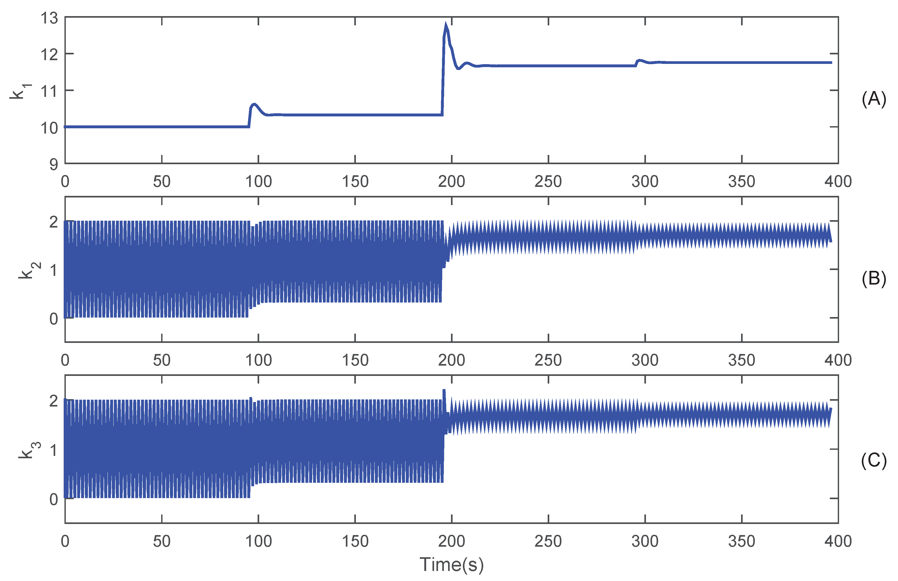
The simulation results are given from Figure 6, Figure 7, Figure 8, Figure 9 and Figure 10. Firstly, the load current is assumed to change as the curve in Figure 6A with three step signals combined. Under the most stringent step signal conditions, the proposed control algorithm presents a favorable control performance, which is shown in Figure 6B. It shows that once there exists a large mutation of the load current, the corresponding oscillations occur on the stack output voltage, yet disappear soon under the proposed control method, and the voltage tends to be stable. The curves of the natural gas flow rate (i.e., the input) and the acceleration are drawn in Figure 7. As can be seen in Figure 7A, the input magnitude constraint generates a saturation phenomenon around Step 200, and the acceleration is within the confining scope. Once the constraints occur, the proposed anti-windup compensator takes effect, as shown in Figure 8A, at the same time to compensate the performance. The Jacobian information and fuel utilization are depicted in Figure 8B,C, which indicates that the fuel utilization is satisfactory within the excellent range under the proposed control strategy. The curves of the exponential PID parameters and the Wiener-type neural network weight coefficients are presented in Figure 9 and Figure 10, respectively.
Moreover, the conventional PID controller is adopted in the simulation in contrast with the proposed control method. The comparisons focus on the following points:
- In Figure 6B, it can be vividly seen that the voltage under PID control has a greater oscillation amplitude and slower convergence speed than the proposed control method.
- In Figure 7A, the natural gas flow rate under PID control is not as stable as the one under the proposed control method when facing the sudden load disturbance.
- In Figure 8C, the fuel utilization under PID control is beyond the permitted scope, which will have a bad effect on the cell life, while the one under the proposed control method is within an appropriate scope.
To summarize, the proposed adaptive tracking constrained control strategy based on the Wiener-type neural network possesses better control performance on the investigated SOFC system in contrast with the PID control with a smaller oscillation amplitude and faster convergence speed and can be applied in the control of nonlinear systems with a complicated dynamics well.
5. Conclusions
In this paper, a new adaptive tracking constrained control strategy based on the online-updated Wiener-type neural network has been proposed for the SOFC, in which we provide a new effective alternative to overcome the control difficulty of the SOFC. Firstly, the nonlinear dynamical model of SOFC is investigated, and the volt-ampere characteristics for the SOFC are presented. Secondly, the dynamic model of the SOFC is approached using the Wiener model formulation, and the parameters of the model are estimated via adaptive Wiener model identification. Thirdly, an adaptive exponential PID controller is designed to achieve the tracking performance of voltage, with an anti-windup compensator utilized to eliminate the harm of saturation considering the input magnitude and rate constraints. Fourthly, the stability of the proposed control system is proven via the Lyapunov function. Finally, the simulation is carried out in the MATLAB/Simulink environment, and the simulation results are analyzed to show that the proposed adaptive tracking constrained control approach possesses good effectiveness when dealing with nonlinear systems with complicated dynamics. Future work will include solving the problem of output constraints, improving our control algorithm to obtain a better tracking performance, and so on.
Author Contributions
All authors contributed to designing and performing measurements, data analysis, scientific discussions, and writing the article.
Funding
This work was partially supported by the National Natural Science Foundation of China (61503156), National Key Research and Development Program (2016YFD0400301), Open Research Fund of Jiangsu Collaborative Innovation Center for Smart Distribution Network, Nanjing Institute of Technology (XTCX201806), National first-class discipline program of Food Science and Technology (JUFSTR20180205), and State Grid Zhejiang Province Technology Project (SGTYHT/17-JS-201)
Conflicts of Interest
The authors declare no conflict of interest, and the founding sponsors had no role in the design of the study, in the collection, analyses or interpretation of data, in the writing of the manuscript, nor in the decision to publish the results.
Abbreviations
The following abbreviations are used in this manuscript:
| Absolute temperature (K) | |
| Faraday’s constant (C/mol) | |
| Universal gas constant () | |
| Ideal standard potential (V) | |
| Number of cells in the stack | |
| Constant, () | |
| Valve molar constant for hydrogen () | |
| Valve molar constant for water () | |
| Valve molar constant for oxygen () | |
| Response time of hydrogen flow (s) | |
| Response time of water flow (s) | |
| Response time of oxygen flow (s) | |
| Ratio of hydrogen to oxygen | |
| r | Ohmic loss () |
| Time constant for the fuel processor (s) | |
| ∂ | Tafel constant |
| Tafel slope | |
| Limiting current density (A) | |
| Partial pressure for hydrogen (Pa) | |
| Partial pressure for water (Pa) | |
| Partial pressure for oxygen (Pa) | |
| Input flow rate for hydrogen (mol/s) | |
| Input flow rate for oxygen (mol/s) | |
| Reacted flow rate for hydrogen (mol/s) | |
| Output flow rate for hydrogen (mol/s) | |
| The stack output voltage (V) | |
| Natural gas flow rate (mol/s) | |
| I | Load current (A) |
| Fuel utilization |
References
- Sendjaja, A.Y.; Kariwala, V. Decentralized control of solid oxide fuel cells. IEEE Trans. Ind. Inform. 2011, 7, 163–170. [Google Scholar] [CrossRef]
- Huang, B.; Qi, Y.T.; Murshed, M. Solid oxide fuel cell: Perspective of dynamic modeling and control. J. Process Control 2011, 21, 1426–1437. [Google Scholar] [CrossRef]
- Allag, T.; Das, T. Robust control of solid oxide fuel cell ultracapacitor hybrid system. IEEE Trans. Control Syst. Technol. 2012, 20, 1–10. [Google Scholar] [CrossRef]
- Jiang, Z.H.; Gao, L.J.; Dougal, R.A. Adaptive control strategy for active power sharing in hybrid fuel cell/battery power sources. IEEE Trans. Energy Convers. 2007, 22, 507–515. [Google Scholar] [CrossRef]
- Sartipizadeh, H.; Vincent, T.L. Robust model predictive control of a catalytic autothermal methane reformer for fuel cell applications. Control Eng. Pract. 2018, 76, 31–40. [Google Scholar] [CrossRef]
- Wu, X.J.; Gao, D.H. Optimal robust control strategy of a solid oxide fuel cell system. J. Power Sources 2018, 374, 225–236. [Google Scholar] [CrossRef]
- Tsourapas, V.; Sun, J.; Stefanopoulou, A. Incremental step reference governor for load conditioning of hybrid fuel cell and gas turbine power plants. IEEE Trans. Control Syst. Technol. 2009, 17, 756–767. [Google Scholar] [CrossRef]
- Li, Y.H.; Choi, S.S.; Rajakaruna, S. An analysis of the control and operation of a solid oxide fuel-cell power plant in an isolated system. IEEE Trans. Energy Convers. 2005, 20, 381–387. [Google Scholar] [CrossRef]
- Hall, D.J.; Colclaser, R.G. Transient modeling and simulation of a tubular solid oxide fuel cell. IEEE Trans. Energy Convers. 1999, 14, 749–753. [Google Scholar] [CrossRef]
- Jurado, F. Modeling SOFC plants on the distribution system using identification algorithms. J. Power Sources 2004, 129, 205–215. [Google Scholar] [CrossRef]
- Xu, D.Z.; Jiang, B.; Liu, F. An improved data driven mdel free adaptive constrained control for a solid oxide fuel cell. IET Control Theory Appl. 2016, 10, 1412–1419. [Google Scholar] [CrossRef]
- Tsourapas, V.; Stefanopoulou, A.G.; Sun, J. Model-based control of an integrated fuel cell and fuel processor with exhaust heat recirculation. IEEE Trans. Control Syst. Technol. 2007, 15, 233–245. [Google Scholar] [CrossRef]
- Vijay, P.; Samantaray, A.K.; Mukherjee, A. A bond graph model-based evaluation of a control scheme to improve the dynamic performance of a solid oxide fuel cell. Mechatronics 2009, 19, 489–502. [Google Scholar] [CrossRef]
- Hajizadeh, A.; Golkar, M.A. Fuzzy neural control of a hybrid fuel cell/battery distributed power generation system. IET Renew. Power Gener. 2009, 3, 402–414. [Google Scholar] [CrossRef]
- Milewski, J.; Swirski, K. Artificial neural network as SOFC model. Rynek Energii 2011, 95, 134–140. [Google Scholar]
- Wu, X.J.; Zhu, X.J.; Cao, G.Y.; Tu, H.Y. Predictive control of SOFC based on a GA-RBF neural network model. J. Power Sources 2008, 179, 232–239. [Google Scholar] [CrossRef]
- Li, S.H.; Wu, F.B.; Li, Q. Identification of Wiener model using dynamic artificial neural networks. J. Power Sources 2000, 17, 92–95. [Google Scholar] [CrossRef]
- Xu, Z.H.; Li, S.F.; Chen, Z.H. A new identification method for the nonlinear systems of Wiener type based on Laguerre functions and static neural networks. J. Syst. Simul. 2002, 14, 1053–1055. [Google Scholar] [CrossRef]
- Zhao, X.D.; Shi, P.; Zheng, X.L.; Zhang, L.X. Adaptive tracking control for switched stochastic nonlinear systems with unknown actuator dead-zone. Automatica 2015, 60, 193–200. [Google Scholar] [CrossRef]
- Tarbouriech, S.; Turner, M. Anti-windup design: an overview of some recent advances and open problems. IET Control Theory Appl. 2009, 3, 1–19. [Google Scholar] [CrossRef] [Green Version]
- Shen, Q.K.; Shi, P. Distributed command filtered backstepping consensus tracking control of nonlinear multiple-agent systems in strict-feedback form. Automatica 2015, 53, 120–124. [Google Scholar] [CrossRef]
- Xu, D.Z.; Jiang, B. A novel model free adaptive control design for multivariable industrial processes. IEEE Trans. Ind. Electron. 2014, 61, 6391–6398. [Google Scholar] [CrossRef]
- Xu, D.Z.; Jiang, B. Adaptive observer based data-driven control for nonlinear discrete-time processes. IEEE Trans. Autom. Sci. Eng. 2014, 11, 1037–1045. [Google Scholar] [CrossRef]
- Li, Y.G.; Shen, J.; Lu, J.H. Constrained model predictive control of a solid oxide fuel cell based on genetic optimization. J. Power Sources 2011, 196, 5873–5880. [Google Scholar] [CrossRef]
- Jurado, F. A method for the identification of solid oxide fuel cells using a Hammerstein model. J. Power Sources 2006, 154, 145–152. [Google Scholar] [CrossRef]
- Zhang, T.J.; Feng, G. Rapid load following of a SOFC power system via stable fuzzy predictive controller. IEEE Trans. Fuzzy Syst. 2009, 17, 357–371. [Google Scholar] [CrossRef]
- Jurado, F. Predictive control of solid oxide fuel cells using fuzzy Hammerstein models. J. Power Sources 2006, 1548, 245–253. [Google Scholar] [CrossRef]
- Kothare, M.V.; Balakrishnan, V.; Morari, M. Robust constrained model predictive control using linear matrix inequalities. Automatica 1996, 32, 1361–1379. [Google Scholar] [CrossRef] [Green Version]
- Lazar, M.; Heemels, W.P.M.H.; Weiland, S.; Bemporad, A. Stabilizing model predictive control of hybrid systems. IEEE Trans. Autom. Control 2006, 51, 1813–1818. [Google Scholar] [CrossRef]
- Wang, X.R.; Huang, B.; Chen, T.W. Data-driven predictive control for solid oxide fuel cells. J. Process Control 2007, 17, 103–114. [Google Scholar] [CrossRef]
- Demircioglu, H.; Yavuzyilmaz, C. Constrained predictive control in continuous time. IEEE Control Syst. 2002, 22, 57–67. [Google Scholar] [CrossRef]
- Voros, J. Modeling and identification of Wiener systems with two-segment nonlinearities. IEEE Trans. Control Syst. Technol. 2003, 11, 253–257. [Google Scholar] [CrossRef]
- Peng, J.Z.; Dubay, R. Identification and adaptive neural network control of a DC motor system with dead-zone characteristics. ISA Trans. 2011, 50, 588–598. [Google Scholar] [CrossRef] [PubMed]
- Xu, D.Z.; Shi, Y.; Ji, Z.C. Model-Free Adaptive Discrete-Time Integral Sliding-Mode-Constrained-Control for Autonomous 4WMV Parking Systems. IEEE Trans. Ind. Electron. 2018, 65, 834–843. [Google Scholar] [CrossRef]
- Rauh, A.; Senkel, L.; Aschemann, H. Interval-based sliding mode control design for solid oxide fuel cells with state and actuator constraints. IEEE Trans. Ind. Electron. 2015, 62, 5208–5217. [Google Scholar] [CrossRef]
Figure 1.
The general structure of the solid oxide fuel cell (SOFC).

Figure 2.
SOFC system dynamic model.

Figure 3.
Volt-ampere characteristics for the SOFC system.

Figure 4.
The structure of the Wiener model.

Figure 5.
Structure of the presented control strategy for SOFC.

Figure 6.
Current load I (A) and the voltage tracking curves of the SOFC of proposed control method compared with the conventional PID control (B).
Figure 6.
Current load I (A) and the voltage tracking curves of the SOFC of proposed control method compared with the conventional PID control (B).

Figure 7.
The curves of the natural gas flow rate (A) and the natural gas flow acceleration (B).

Figure 8.
Anti-windup compensation signal (A), Jacobian information (B) and fuel utilization for the proposed control method compared with conventional PID control (C).
Figure 8.
Anti-windup compensation signal (A), Jacobian information (B) and fuel utilization for the proposed control method compared with conventional PID control (C).

Figure 9.
The curves of exponential PID parameters.

Figure 10.
The curves of the Wiener-type neural network weight coefficients.


Table 1.
Parameters of the SOFC system model.
| Parameter | Value | Parameter | Value |
|---|---|---|---|
| 1273 | 26.1 | ||
| 96,485 | 78.3 | ||
| 8.314 | 2.91 | ||
| 1.18 | 1.145 | ||
| 384 | r | 0.126 | |
| 5 | |||
| ∂ | 0.05 | ||
| 0.11 | |||
| 800 |
© 2018 by the authors. Licensee MDPI, Basel, Switzerland. This article is an open access article distributed under the terms and conditions of the Creative Commons Attribution (CC BY) license (http://creativecommons.org/licenses/by/4.0/).
Share and Cite
MDPI and ACS Style
Xia, Y.; Zou, J.; Yan, W.; Li, H. Adaptive Tracking Constrained Controller Design for Solid Oxide Fuel Cells Based on a Wiener-Type Neural Network. Appl. Sci. 2018, 8, 1758. https://0-doi-org.brum.beds.ac.uk/10.3390/app8101758
AMA Style
Xia Y, Zou J, Yan W, Li H. Adaptive Tracking Constrained Controller Design for Solid Oxide Fuel Cells Based on a Wiener-Type Neural Network. Applied Sciences. 2018; 8(10):1758. https://0-doi-org.brum.beds.ac.uk/10.3390/app8101758
Chicago/Turabian StyleXia, Yan, Jianxiao Zou, Wenxu Yan, and Huayin Li. 2018. "Adaptive Tracking Constrained Controller Design for Solid Oxide Fuel Cells Based on a Wiener-Type Neural Network" Applied Sciences 8, no. 10: 1758. https://0-doi-org.brum.beds.ac.uk/10.3390/app8101758
Note that from the first issue of 2016, this journal uses article numbers instead of page numbers. See further details here.