Unified Friction Formulation from Laminar to Fully Rough Turbulent Flow


1
European Commission, Joint Research Centre (JRC), Directorate C—Energy, Transport and Climate, Unit C3: Energy Security, Distribution and Markets, Via Enrico Fermi 2749, 21027 Ispra (VA), Italy
2
Alfatec, Bulevar Nikole Tesle 63/5, 18000 Niš, Serbia
3
IT4Innovations National Supercomputing Center, VŠB—Technical University of Ostrava, 17. listopadu 2172/15, 708 00 Ostrava, Czech Republic
*
Authors to whom correspondence should be addressed.
Appl. Sci. 2018, 8(11), 2036; https://0-doi-org.brum.beds.ac.uk/10.3390/app8112036
Submission received: 14 September 2018
/
Revised: 2 October 2018
/
Accepted: 20 October 2018
/
Published: 24 October 2018
(This article belongs to the Section Mechanical Engineering)
Abstract
:This paper provides a new unified formula for Newtonian fluids valid for all pipe flow regimes from laminar to fully rough turbulent flow. This includes laminar flow; the unstable sharp jump from laminar to turbulent flow; and all types of turbulent regimes, including the smooth turbulent regime, the partial non-fully developed turbulent regime, and the fully developed rough turbulent regime. The new unified formula follows the inflectional form of curves suggested in Nikuradse’s experiment rather than the monotonic shape proposed by Colebrook and White. The composition of the proposed unified formula uses switching functions and interchangeable formulas for the laminar, smooth turbulent, and fully rough turbulent flow regimes. Thus, the formulation presented below represents a coherent hydraulic model suitable for engineering use. This new flow friction model is more flexible than existing literature models and provides smooth and computationally cheap transitions between hydraulic regimes.
1. Introduction
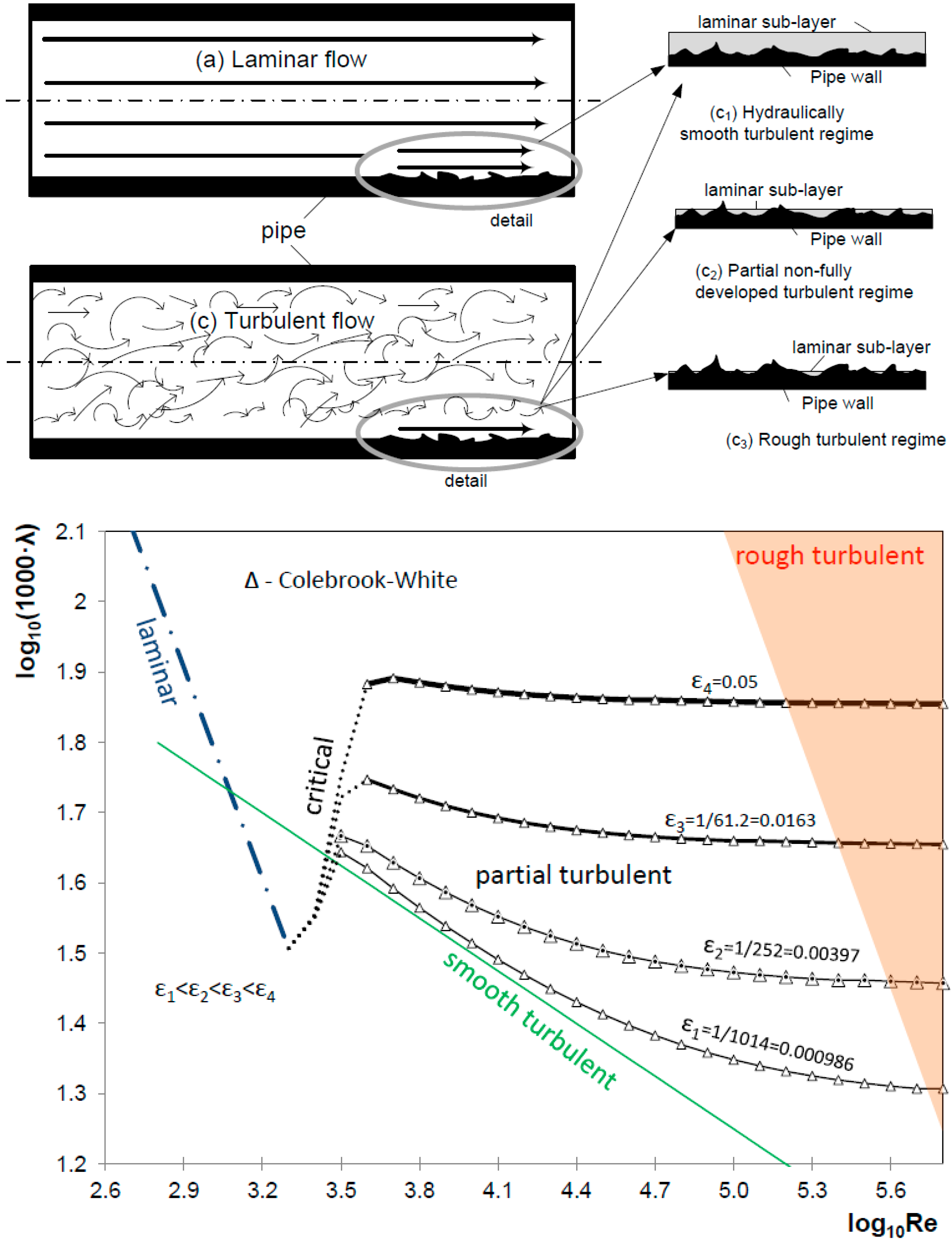
In the field of hydraulics, resistance in pipe flow is usually represented by the Darcy flow friction factor λ, which depends on the Reynolds number Re and the relative roughness of the inner pipe surface ε [1]. All three quantities are dimensionless. For pipe flow, the Reynolds number Re usually takes values between 0 and 108, while the relative roughness of the inner pipe surface ε ranges from 0 to 0.05. A pipe’s material, as well as its condition, is characterized by the relative roughness of the inner pipe surface, but also depends on the hydraulic flow regime ruled by the thickness of a thin laminar boundary sublayer of fluid near the inner pipe surface [2,3] (Figure 1(top)). In general, several different hydraulic regimes can occur during pipe flow (Figure 1): the laminar regime , the sharp transition from the laminar regime to the smooth turbulent regime , the smooth turbulent regime , the non-fully developed partially turbulent regime , and the fully developed rough turbulent regime .
, the laminar regime is characterized by the absence of vortices, while the roughness of the inner pipe surface does not have flow effects. , the transition from the laminar regime to the turbulent regime is sharp and almost immediate, so it can be described by a sudden increase in the friction factor λ. The turbulent regimes in are characterized by higher values of the Reynolds number Re, with vortices in flow. In , the smooth turbulent regime is characterized by vortices in the middle of the pipe, while in the roughness of the inner pipe surface is covered by the laminar sublayer. In , with an increase of the Reynolds number Re, the thickness of the laminar sublayer decreases, and the roughness of the inner pipe surface becomes important. Thus, in the fully developed rough turbulent flow regime, the roughness of the inner pipe surface plays a dominant role.
Figure 1(top) includes a physical interpretation of the different hydraulic regimes, while Figure 1(bottom) contains related diagrams.
Similar to Figure 1, the widely-known Moody diagram [4,5,6] provides a representation of different hydraulic regimes. The turbulent part of the Moody diagram is based on the Colebrook equation [7].
While the formula for the laminar regime is theoretical, the formulas for all types of turbulent regimes are empirical [8,9,10]. Although coherent unified models for all hydraulic regimes exist [11,12,13], they are not as flexible as the model presented here because they are fixed (i.e., they do not allow changing separate formulas valid for different hydraulic regimes). In contrast, the unified formula presented here allows any of the formulas for a particular hydraulic regime to be included: one for the laminar regime , one for the hydraulically smooth turbulent regime and one for the fully developed rough turbulent regime . Thus, the unified formula presented here uses three switching functions—, and —to provide a smooth transition between hydraulic regimes, as seen in Equations (7)–(9) of this paper. The proposed unified formula is contained in Equation (1):
In Equation (1), , and represent switching functions; (a) is a formula for laminar flow, ; is for smooth turbulent flow, ; and is for fully developed rough turbulent flow, . Here, Re is the Reynolds number, ε is the relative roughness of the inner pipe surface, and ζ and ς are functional symbols. Functions ζ and ς are empirical; related equations are available from the literature [14].
The proposed unified formula follows the inflectional shape of the flow friction curve suggested in Nikuradse’s experiment [8,15] rather than the monotonic curve shape proposed by Colebrook and White [7,9]. In the instant case, the curve shape is formed through careful fitting of the switching functions , and . Recent experiments using flow friction factors [14] at Princeton and Oregon have confirmed Nikuradse’s inflectional curve shape; the experiments reached similar conclusions although the two experiments differed significantly. The Princeton facility used compressed air, while Oregon used helium, oxygen, nitrogen, carbon dioxide, and sulfur hexafluoride. The Princeton device weighed approximately 25 tons, whereas the Oregon device weighed approximately 0.7 kg. A variant of the Moody diagram, which includes Nikuradse’s inflectional curve shape, also exists [16].
2. Previous Works and the Source of Their Differences
In Equations (2)–(4), λ is the Darcy friction factor, Re is the Reynolds number, and ε is the relative roughness of the inner pipe surface (all three quantities are dimensionless).
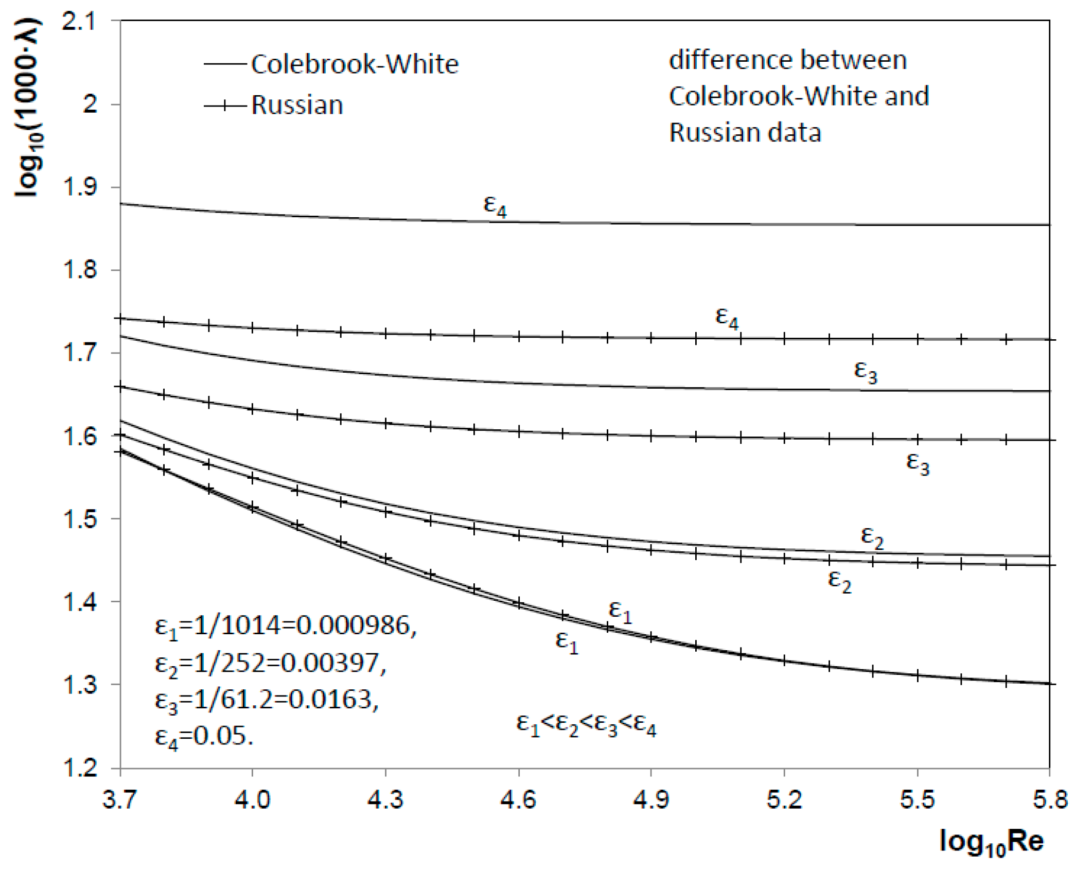
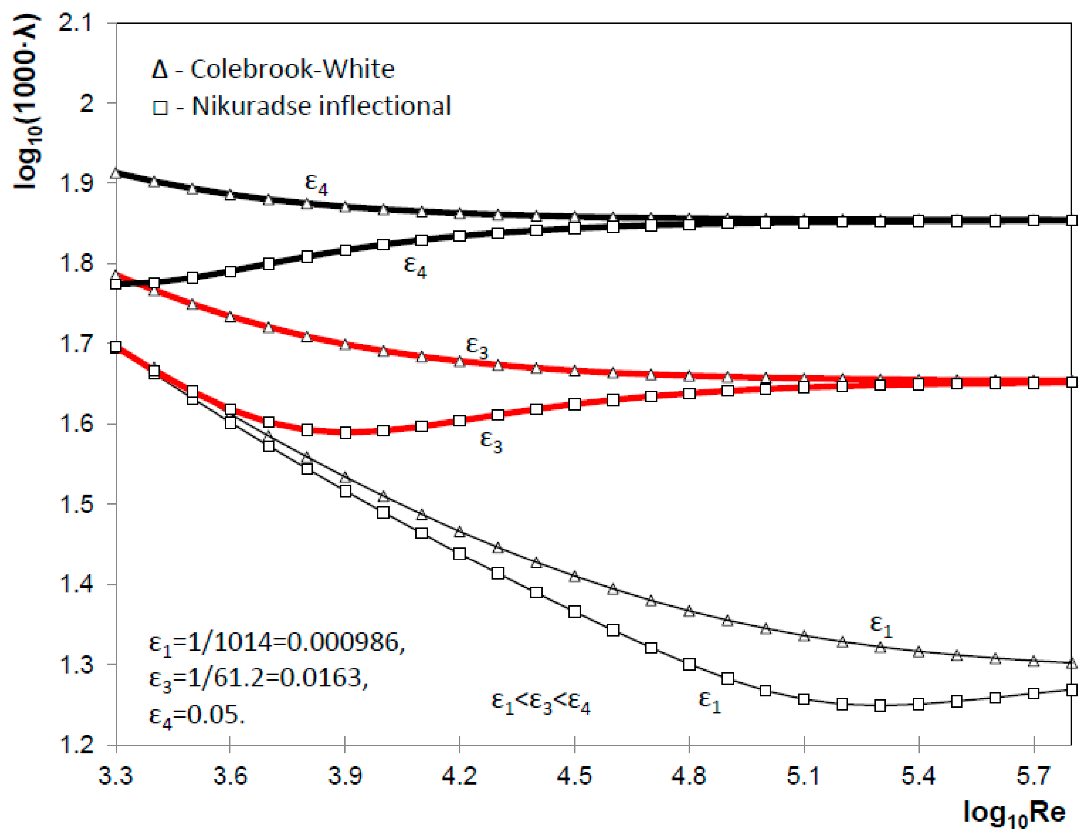
The turbulent parts of Equations (2) and (3) are based on the Colebrook formula [7], while Equation (4) is based on formulas from Russian engineering practice [17]. The turbulent part of Equation (2) [11] is based on the Churchill approximation of the Colebrook equation [18], while Equation (3) [12] is based on approximations of the Colebrook equation given by Swamee and Jain [19]. As shown in Figure 2, formulas from Russian practices and those based on the Colebrook equation yield almost identical results for low values of relative roughness ε; in the case of higher values of relative roughness ε, formulas from Russian practice give lower values for the flow friction factor λ compared with the Colebrook equation. Both the Colebrook equation and formulas from Russian practice have a monotonic shape of flow friction curves (Figure 2), which is disputed not only by new experiments such as those from the Princeton and Oregon laboratories [15], but also by an older Nikuradse experiment [8]. The Nikuradse experiment was conducted in 1932 and 1933, while the Colebrook and White experiment was reported in 1937 [9]). The Nikuradse experiment proposed a shape of curves in the turbulent regime as intervals of declining values of the friction factor λ before they reached the final maximal values for the fully developed rough turbulent flow. This property of flow friction factors is known as Nikuradse’s inflectional shape of transition to the fully turbulent regime, as seen in Figure 3 [20,21].
The currently available formulas valid for all hydraulic regimes, Equations (2)–(4), do not follow Nikuradse’s inflectional law. The Colebrook equation can be extended to fit the measured data from Nikuradse’s experiment, as seen in Equation (5) [16]:
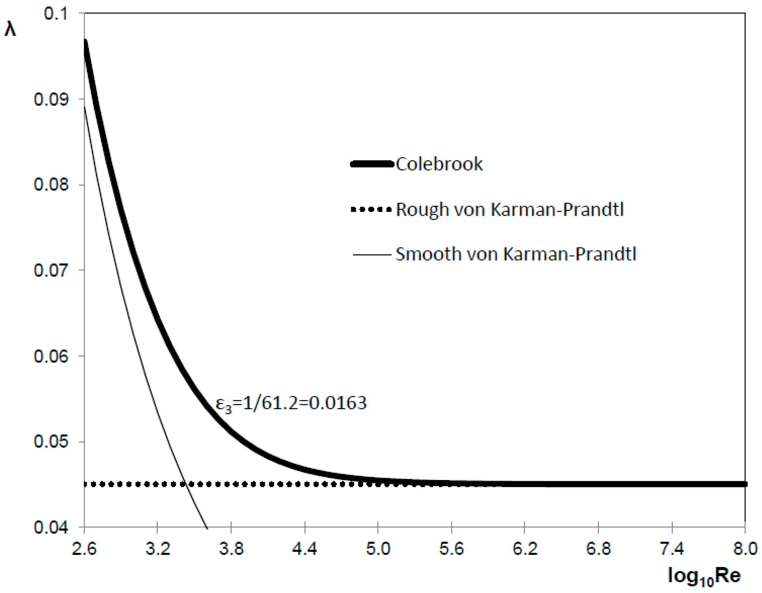
In Equation (5), e is an exponential function, where E = 0 gives the Colebrook equation without the Nikuradse extension. The Colebrook equation is given in the implicit form with respect to the flow friction factor λ [22,23,24,25], while the formulas from Russian practice are primarily given in explicit power-law types of expressions [26]. As shown in Figure 4, the Colebrook equation is developed to unify the von Karman–Prandtl equations for both smooth turbulent flow and fully rough flow in a smooth, asymptotic way. Equation (6) is as follows, keeping in mind that :
In Equation (6), represents smooth turbulent flow, represents transitional non-fully developed turbulent flow, and represents fully developed rough turbulent flow. Similar strategies to unify and modify the equation to conform to certain laws (in our case Nikuradse’s inflectional law) are used for our unified equation, as seen in Equation (1). On the other hand, Colebrook [9] (see Equations (5) and (6)) uses a logarithmic law to unify and in . In our approach, we use switching functions , and to unify , and in one coherent hydraulic model, where represents the laminar regime, as previously explained by Equation (1).
3. Switching Functions, Friction Factors, New Formulation, and Comparative Analysis
Required inputs for our unified formula, Equation (1), are shown here, including: switching functions , and and formulas for friction factors for the hydraulic zones laminar flow , smooth turbulent flow , and fully developed rough turbulent flow .
3.1. Switching Functions
The unified formula valid for all hydraulic cases depends directly on the switching functions , and . Switching functions provide for a smooth transition between different hydraulic regimes. A connection of curves created by separate formulas for laminar flow , smooth turbulent flow , and fully developed rough turbulent flow , is not smooth without help from the carefully selected switching functions , and . These three functions are rational and generated in HeuristicLab, a software environment for heuristic and evolutionary algorithms [27]. The proposed switching functions have a simple form and therefore can be incorporated easily into computer codes without any significant burden on the Central Processing Unit [28]. The proposed switching functions , and are respectively represented by Equations (7)–(9) and Figure 5, Figure 6 and Figure 7:
In Equations (7)–(9), symbols , and denote switching functions.
3.2. Friction Factors
Friction factors, which serve as inputs for the unified formula presented in Equation (1), will be explicated here in further detail. Specifically, we will present friction factors for laminar flow , smooth turbulent flow , and fully developed rough turbulent flow hydraulic regimes. Turbulent flow is a phenomena that still causes a stir among experts [29,30]. Thus, the formula shown here is suitable for the flow of Newtonian fluids, whereas some restrictions are applied for gases [31].
3.2.1. Laminar Flow
Due to the overriding effect of viscosity forces in laminar flow, even rough inner pipe surface appears to be hydraulically smooth for Reynolds numbers lower than about 3000. Consequently, the roughness of walls, unless significant, does not affect the flow resistance. Under these conditions of flow, the friction coefficient λ is always a function of the Reynolds number Re alone, as seen in Equation (10):
3.2.2. Smooth Turbulent Flow
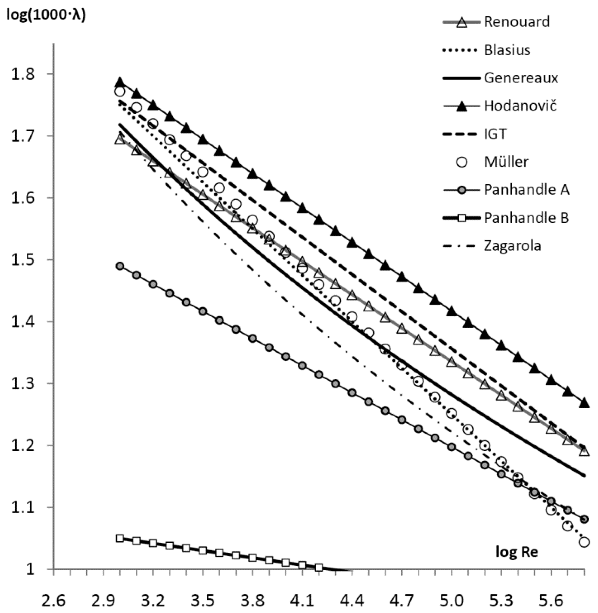
In the hydraulically smooth regime, the friction factor λ is only a function of the Reynolds number Re, and the resistance to flow is independent of the inner pipe surface relative roughness ε. This regime is restricted to relatively small values of the Reynolds number Re, where the roughness of the inner pipe surface is completely hidden in the laminar boundary sublayer. The literature on the hydraulically smooth regime abounds with reliable friction factor equations. In general, with some extensions and modifications, there are Blasius-form relationships (power-law relationships), as seen in Equation (11)-up, and von Karman–Prandtl-form relationships (logarithmic relationships), as seen in Equation (11)-down:
Some possible values for coefficient A and exponent B in Blasius-form power-law relationships [17,26,31], as seen in Equation (11), are given in Table 1 below:
With regard to von Karman–Prandtl-form logarithmic relationships, the below displays their basic form, which is used in a smooth part of the Colebrook equation, as seen in Equation (12). This formula is an updated version of that given by McKeon et al. [32], seen in Equation (12):
In addition, for the hydraulically smooth turbulent regime, among others, it is possible to use Equation (13)—by Genereaux, Leese, Nikuradse, Hermann, White, and Konakov [17,26,31]—from top to bottom:
Though the Blasius-form power-law relationships, as seen in Equation (11)-up, have the merit of simplicity, they also have certain disadvantages; one of these disadvantages is that the relationships can only be applied over a limited range of hydraulically smooth regimes. Extrapolations beyond this range cannot be made with confidence. Figure 8 gives a comparison of some of the friction coefficients λ used in the hydraulically smooth turbulent regime. The friction factor λ corresponding to the Hodanovič equation has higher values than those in Panhandle B, as seen in Table 1. This demonstrates the limits of the application of several of the available equations, as many of them were developed for particular situations. For example, Panhandle B is valid for large-diameter pipelines, while Renoard is suitable for the distribution of PVC pipeline networks in urban areas. In addition, the main constraint in using von Karman–Prandtl-form logarithmic relationships, as seen in Equation (11)-down, is their implicit form with respect to flow friction λ.
3.2.3. Fully Developed Rough Turbulent Flow
At high values of the Reynolds number Re, the friction factor λ becomes a constant for a given relative roughness ε [33]. In the case of fully rough turbulent flow, the laminar sublayer near the pipe wall practically does not exist, and thus the flow is dominated by the relative roughness ε. The equation can either be logarithmic, as seen in Equation (14), or power-law, as used predominantly in Russian engineering practice (such as in Altshul- or Shifrinson-type formulas), as seen in Equation (14) [17]:
Figure 2 of this paper displays a difference in results with regard to Equation (14).
3.3. New Unified Flow Friction Formulation
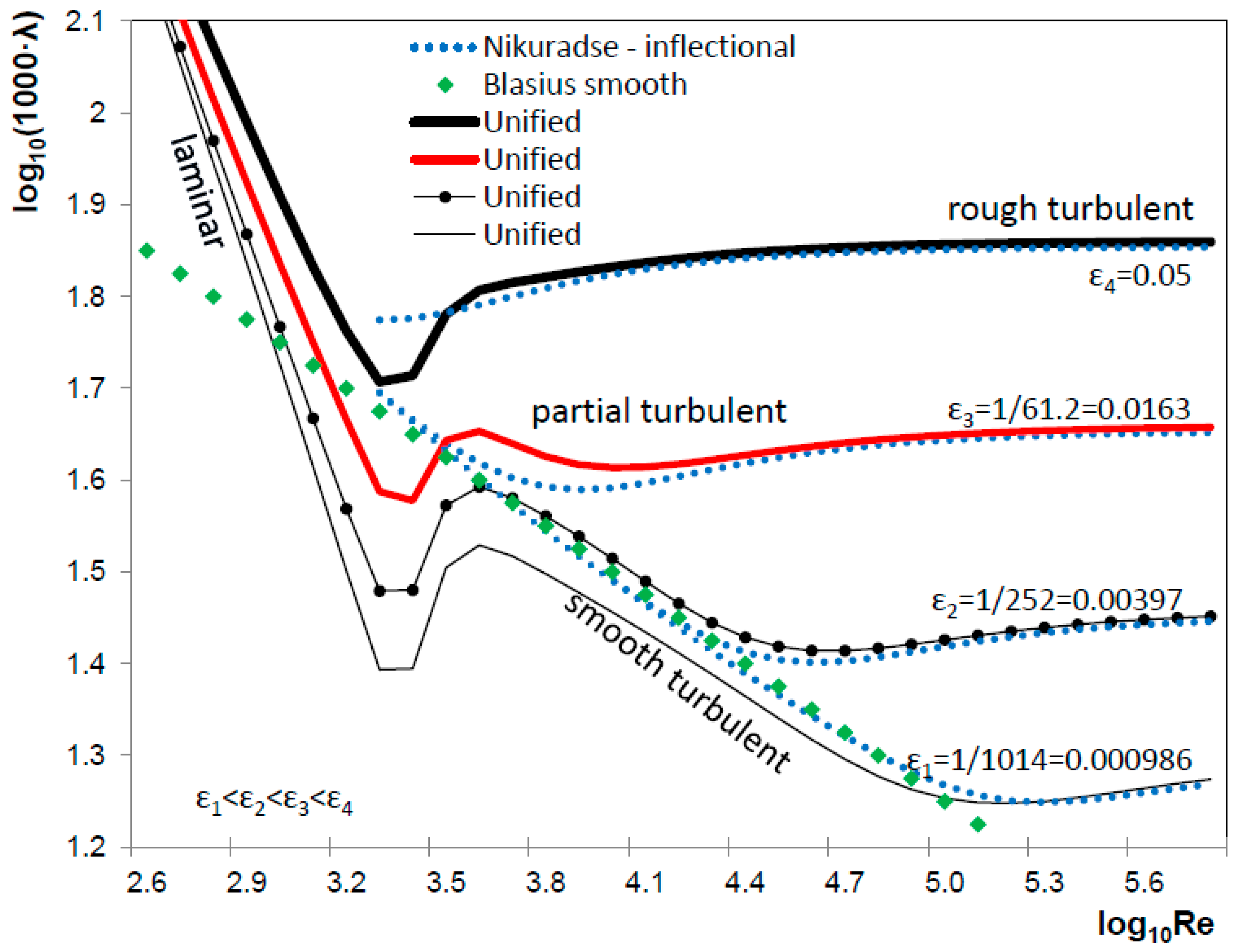
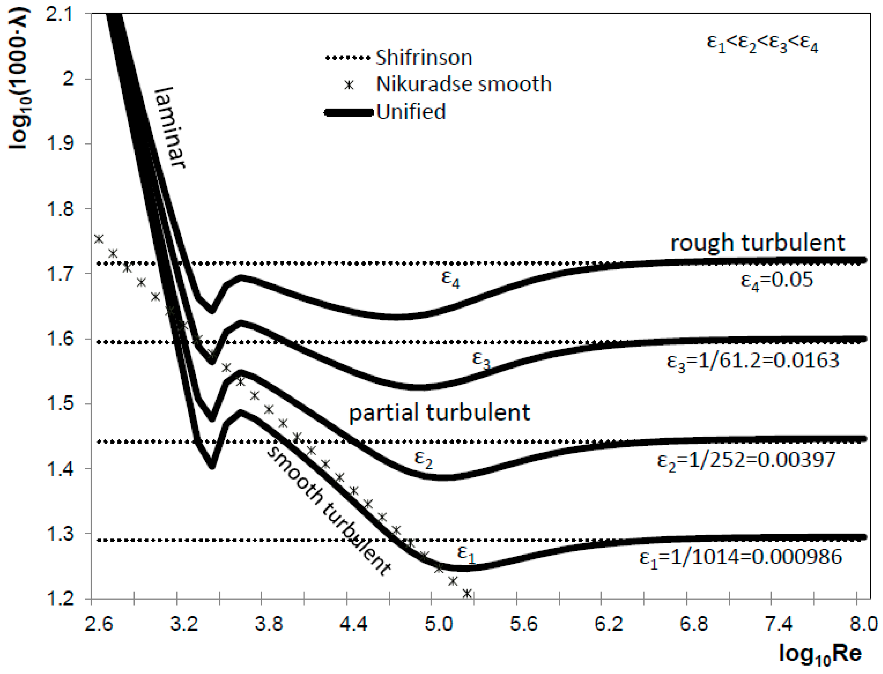
A novel formula for all hydraulic regimes is developed in order to easily encapsulate separate formulas for different hydraulic regimes into one coherent hydraulic regime. The structure of the proposed formula, , is based on using three switching functions—, and —and formulas for laminar flow , smooth turbulent flow , and fully developed rough turbulent flow . Consequently, all hydraulic regimes can be simulated in one simple formula that includes a sharp transition from the laminar to the smooth turbulent and the non-fully developed partially turbulent regimes . As already explained, the switching functions are set in such a way so as to always produce Nikuradse’s inflectional curve shape [34]. Two possible encapsulations in the unified coherent hydraulic model are given in Equation (15), with related diagrams contained in Figure 9 and Figure 10:
In Figure 9, the shape outlined by the blue dots results from using the Colebrook equation with the extension for Nikuradse’s inflectional law from Equation (5). Laminar flow is comprised of , whereas the hydraulically smooth turbulent regime with the Blasius expression is represented as . Finally, the fully developed turbulent regime with the von Karman–Prandtl equation can be seen in Equation (15)-I. In Figure 10, a similar approach is outlined using different formulas, as indicated in Equation (15)-II.
Using the same separate formulas for different hydraulic regimes from Equation (15), the following additional encapsulation is also possible, seen in Equation (16):
Using this method, and after performing numerical tests, the most appropriate equation (comprised of separate available formulas for different hydraulic regimes) can be optimally encapsulated depending upon the particular circumstances of each engineering project.
4. Conclusions
A sudden failure of valves or other components related to hydraulic systems in civil and mechanical engineering [35,36,37] can also cause a change of flow regime. Because of this, it is crucial to take such cases into consideration. The unified flow friction approach presented here is flexible, as proposed equations for a certain hydraulic flow regime can be easily altered using interchangeable formulas for laminar, smooth turbulent, and rough turbulent flow. Although our previous experiences with artificial intelligence [38,39,40] have shown that an encapsulation of all flow friction regimes into one coherent model is not a straightforward task, the form proposed here is simple. Thus, the unified approach presented here can be easily implemented with software codes. Moreover, as the proposed switching functions are carefully chosen so that they follow Nikuradse’s inflectional law of roughness, our unified approach seems to be more realistic than the classic implicitly-given 80-year-old Colebrook–White monotonic curves model [41,42,43,44,45,46]. The switching functions presented here are expressed by simple rational functions and thus do not contain computationally expensive transcendental functions. Consequently, our unified flow friction formulation possesses a reasonable computational complexity.
Author Contributions
This paper is a joint effort by the authors, who worked together on models of natural gas distribution networks. P.P. has a scientific background in applied mathematics and programming, while D.B.’s background is in control and applied computing in mechanical and petroleum engineering. Based on the idea of D.B., P.P. used numerical data provided by D.B. to develop the presented switching functions in HeuristicLab [computer software]. D.B. prepared figures and wrote the draft of this article.
Funding
Resources to cover the Article Processing Charge were provided by the European Commission. This paper is registered in the internal system for publication of the European Commission; Pubsy as JRC113382.
Acknowledgments
Part of the research is from the project iii44006 of the Ministry of Education, Science and Technological Development of the Republic of Serbia.
Conflicts of Interest
The authors declare no conflicts of interest. Affiliated organizations, nor any person acting on their behalf is responsible for the use of this publication.
Nomenclature
The following symbols are used in this paper:
| λ | Darcy friction factor (Moody, Darcy–Weisbach, or Colebrook); dimensionless |
| Re | Reynolds number; dimensionless |
| ε | relative roughness of inner pipe surface; dimensionless |
| laminar | |
| smooth turbulent | |
| non-fully developed partially turbulent | |
| fully developed rough turbulent | |
| , and | switching functions |
| e | exponential function |
| Log | logarithmic function |
| Ln | Napier natural logarithm |
| A, B, C, D and E | auxiliary terms |
References
- Brown, G.O. Henry Darcy and the making of a law. Water Resour. Res. 2002, 38, 11. [Google Scholar] [CrossRef]
- Brkić, D. Can pipes be actually really that smooth? Int. J. Refrig. 2012, 35, 209–215. [Google Scholar] [CrossRef] [Green Version]
- Shojaeizadeh, A.; Safaei, M.R.; Alrashed, A.A.; Ghodsian, M.; Geza, M.; Abbassi, M.A. Bed roughness effects on characteristics of turbulent confined wall jets. Measurement 2018, 122, 325–338. [Google Scholar] [CrossRef]
- Moody, L.F. Friction factors for pipe flow. Trans. ASME 1944, 66, 671–684. [Google Scholar]
- LaViolette, M. On the history, science, and technology included in the Moody diagram. J. Fluids Eng. 2017, 139, 030801. [Google Scholar] [CrossRef]
- Flack, K.A. Moving beyond Moody. J. Fluid Mech. 2018, 842, 1–4. [Google Scholar] [CrossRef] [Green Version]
- Colebrook, C.F. Turbulent flow in pipes with particular reference to the transition region between the smooth and rough pipe laws. J. Inst. Civ. Eng. 1939, 11, 133–156. [Google Scholar] [CrossRef]
- Nikuradse, J. Laws of Flow in Rough Pipes; National Advisory Committee for Aeronautics: Washington, DC, USA, 1950; (Version in German from 1933: “Stromungsgesetze in Rauhen Rohren”). Available online: http://ntrs.nasa.gov/archive/nasa/casi.ntrs.nasa.gov/199300939381993093938.pdf (accessed on 15 September 2018).
- Colebrook, C.; White, C. Experiments with fluid friction in roughened pipes. Proc. R. Soc. Lond. Ser. A Math. Phys. Sci. 1937, 161, 367–381. [Google Scholar] [CrossRef] [Green Version]
- Allen, J.J.; Shockling, M.A.; Kunkel, G.J.; Smits, A.J. Turbulent flow in smooth and rough pipes. Philos. Trans. R. Soc. Lond. A Math. Phys. Eng. Sci. 2007, 365, 699–714. [Google Scholar] [CrossRef] [PubMed] [Green Version]
- Churchill, S.W. Friction-factor equation spans all fluid flow regimes. Chem. Eng. 1977, 84, 91–92. [Google Scholar]
- Swamee, P.K. Design of a submarine oil pipeline. J. Transp. Eng. 1993, 119, 159–170. [Google Scholar] [CrossRef]
- Чepникин, B.A.; Чepникин, A.B. Oбобщeннaя φоpмyлa для pacчeтa коэφφициeнтa гидpaвличecкого cопpотивлeния мaгиcтpaльныx тpyбопpоводов для cвeтлыx нeφтeпpодyктов и мaловязкиx нeφтeй. Hayкa и тexнологии тpyбопpоводного тpaнcпоpтa нeφти и нeφтeпpодyктов 2012, 4, 64–66. Available online: http://transenergostroy.ru/publications/src/20130424/Chernikin_gidrav_soprotivlenie.pdf (accessed on 23 October 2018). (In Russian).
- Joseph, D.D.; Yang, B.H. Friction factor correlations for laminar, transition and turbulent flow in smooth pipes. Phys. D Nonlinear Phenom. 2010, 239, 1318–1328. [Google Scholar] [CrossRef] [Green Version]
- Yang, B.H.; Joseph, D.D. Virtual Nikuradse. J. Turbul. 2009, 10, N11. [Google Scholar] [CrossRef]
- McGovern, J. Friction Factor Diagrams for Pipe Flow. 2011. Available online: https://arrow.dit.ie/engschmecart/28/ (accessed on 15 September 2018).
- Aльтшyль, A.Д. Гидpaвличecкиe Cопpотивлeния; Heдpa: Moscow, Russia, 1982. (In Russian) [Google Scholar]
- Churchill, S.W. Empirical expressions for the shear stress in turbulent flow in commercial pipe. AIChE J. 1973, 19, 375–376. [Google Scholar] [CrossRef]
- Swamee, P.K.; Jain, A.K. Explicit equations for pipe flow problems. J. Hydraul. Div. ASCE 1976, 102, 657–664. [Google Scholar]
- Sletfjerding, E.; Gudmundsson, J.S. Friction factor directly from roughness measurements. J. Energy Resour. Technol. 2003, 125, 126–130. [Google Scholar] [CrossRef]
- Shockling, M.A.; Allen, J.J.; Smits, A.J. Roughness effects in turbulent pipe flow. J. Fluid Mech. 2006, 564, 267–285. [Google Scholar] [CrossRef]
- Brkić, D. Review of explicit approximations to the Colebrook relation for flow friction. J. Pet. Sci. Eng. 2011, 77, 34–48. [Google Scholar] [CrossRef] [Green Version]
- Praks, P.; Brkić, D. Advanced iterative procedures for solving the implicit Colebrook equation for fluid flow friction. Adv. Civ. Eng. 2018, 2018, 5451034. [Google Scholar] [CrossRef]
- Praks, P.; Brkić, D. Choosing the optimal multi-point iterative method for the Colebrook flow friction equation. Processes 2018, 6, 130. [Google Scholar] [CrossRef]
- Praks, P.; Brkić, D. One-log call iterative solution of the Colebrook equation for flow friction based on Padé polynomials. Energies 2018, 11, 1825. [Google Scholar] [CrossRef]
- Brkić, D. A gas distribution network hydraulic problem from practice. Pet. Sci. Technol. 2011, 29, 366–377. [Google Scholar] [CrossRef]
- Wagner, S.; Kronberger, G.; Beham, A.; Kommenda, M.; Scheibenpflug, A.; Pitzer, E.; Vonolfen, S.; Kofler, M.; Winkler, S.; Dorfer, V.; et al. Architecture and design of the HeuristicLab optimization environment. Top. Intell. Eng. Inform. 2014, 6, 197–261. [Google Scholar] [CrossRef]
- Vatankhah, A.R. Approximate analytical solutions for the Colebrook equation. J. Hydraul. Eng. 2018, 144, 06018007. [Google Scholar] [CrossRef]
- Cipra, B. A new theory of turbulence causes a stir among experts. Science 1996, 272, 951. [Google Scholar] [CrossRef]
- Chandrasekhar, S.; Sharma, V.M. Brownian heat transfer enhancement in the turbulent regime. Facta Univ. Ser. Mech. Eng. 2016, 14, 169–177. [Google Scholar] [CrossRef]
- Bagajewicz, M.; Valtinson, G. Computation of natural gas pipeline hydraulics. Ind. Eng. Chem. Res. 2014, 53, 10707–10720. [Google Scholar] [CrossRef]
- McKeon, B.J.; Swanson, C.J.; Zagarola, M.V.; Donnelly, R.J.; Smits, A.J. Friction factors for smooth pipe flow. J. Fluid Mech. 2004, 511, 41–44. [Google Scholar] [CrossRef] [Green Version]
- Brkić, D. A note on explicit approximations to Colebrook’s friction factor in rough pipes under highly turbulent cases. Int. J. Heat Mass Transf. 2016, 93, 513–515. [Google Scholar] [CrossRef]
- Thakkar, M.; Busse, A.; Sandham, N.D. Direct numerical simulation of turbulent channel flow over a surrogate for Nikuradse-type roughness. J. Fluid Mech. 2018, 837, R1. [Google Scholar] [CrossRef]
- Nikolić, B.; Jovanović, M.; Milošević, M.; Milanović, S. Function k-as a link between fuel flow velocity and fuel pressure, depending on the type of fuel. Facta Univ. Ser. Mech. Eng. 2017, 15, 119–132. [Google Scholar] [CrossRef]
- Praks, P.; Kopustinskas, V.; Masera, M. Monte-Carlo-based reliability and vulnerability assessment of a natural gas transmission system due to random network component failures. Sustain. Resilient Infrastruct. 2017, 2, 97–107. [Google Scholar] [CrossRef]
- Praks, P.; Kopustinskas, V.; Masera, M. Probabilistic modelling of security of supply in gas networks and evaluation of new infrastructure. Reliab. Eng. Syst. Saf. 2015, 144, 254–264. [Google Scholar] [CrossRef]
- Brkić, D.; Ćojbašić, Ž. Intelligent flow friction estimation. Comput. Intell. Neurosci. 2016, 2016, 5242596. [Google Scholar] [CrossRef] [PubMed]
- Brkić, D.; Ćojbašić, Ž. Evolutionary optimization of Colebrook’s turbulent flow friction approximations. Fluids 2017, 2, 15. [Google Scholar] [CrossRef]
- Praks, P.; Brkić, D. Symbolic regression-based genetic approximations of the Colebrook equation for flow friction. Water 2018, 10, 1175. [Google Scholar] [CrossRef]
- Uršič, M.; Kompare, B. Improvement of the hydraulic friction losses equations for flow under pressure in circular pipes. Acta Hydrotech. 2003, 21, 57–74. [Google Scholar]
- Bellos, V.; Nalbantis, I.; Tsakiris, G. Friction modeling of flood flow simulations. J. Hydraul. Eng. 2018, 144, 04018073. [Google Scholar] [CrossRef]
- Cheng, N.S. Formulas for friction factor in transitional regions. J. Hydraul. Eng. 2008, 134, 1357–1362. [Google Scholar] [CrossRef]
- Brkić, D. Discussion of “Economics and Statistical Evaluations of Using Microsoft Excel Solver in Pipe Network Analysis” by I. A. Oke, A. Ismail, S. Lukman, S. O. Ojo, O. O. Adeosun, and M. O. Nwude. J. Pipeline Syst. Eng. 2018, 9, 07018002. [Google Scholar] [CrossRef]
- Eck, B.J. Use of a smoothed model for pipe friction loss. J. Hydraul. Eng. 2016, 143, 06016022. [Google Scholar] [CrossRef]
- Basse, N.T. Turbulence intensity and the friction factor for smooth- and rough-wall pipe flow. Fluids 2017, 2, 30. [Google Scholar] [CrossRef]
Figure 1.
Hydraulic regimes for pipe flow: the laminar regime , the sharp transition from the laminar regime to the smooth turbulent regime (critical) , the smooth turbulent regime , the non-fully developed partially turbulent regime and the fully developed rough turbulent regime . (top) contains physical interpretations, while (bottom) contains related diagrams.

Figure 2.
Different values of the flow friction factor obtained using the Colebrook formula versus the formulas from Russian practice.
Figure 2.
Different values of the flow friction factor obtained using the Colebrook formula versus the formulas from Russian practice.

Figure 3.
Different shapes of flow friction factor curves obtained using the Colebrook formula versus those that follow Nikuradse’s inflectional law.
Figure 3.
Different shapes of flow friction factor curves obtained using the Colebrook formula versus those that follow Nikuradse’s inflectional law.

Figure 4.
Von Karman–Prandtl equations for smooth turbulent flow and for fully rough turbulent flow unified by Colebrook using a logarithmic function in the one coherent hydraulic model.
Figure 4.
Von Karman–Prandtl equations for smooth turbulent flow and for fully rough turbulent flow unified by Colebrook using a logarithmic function in the one coherent hydraulic model.

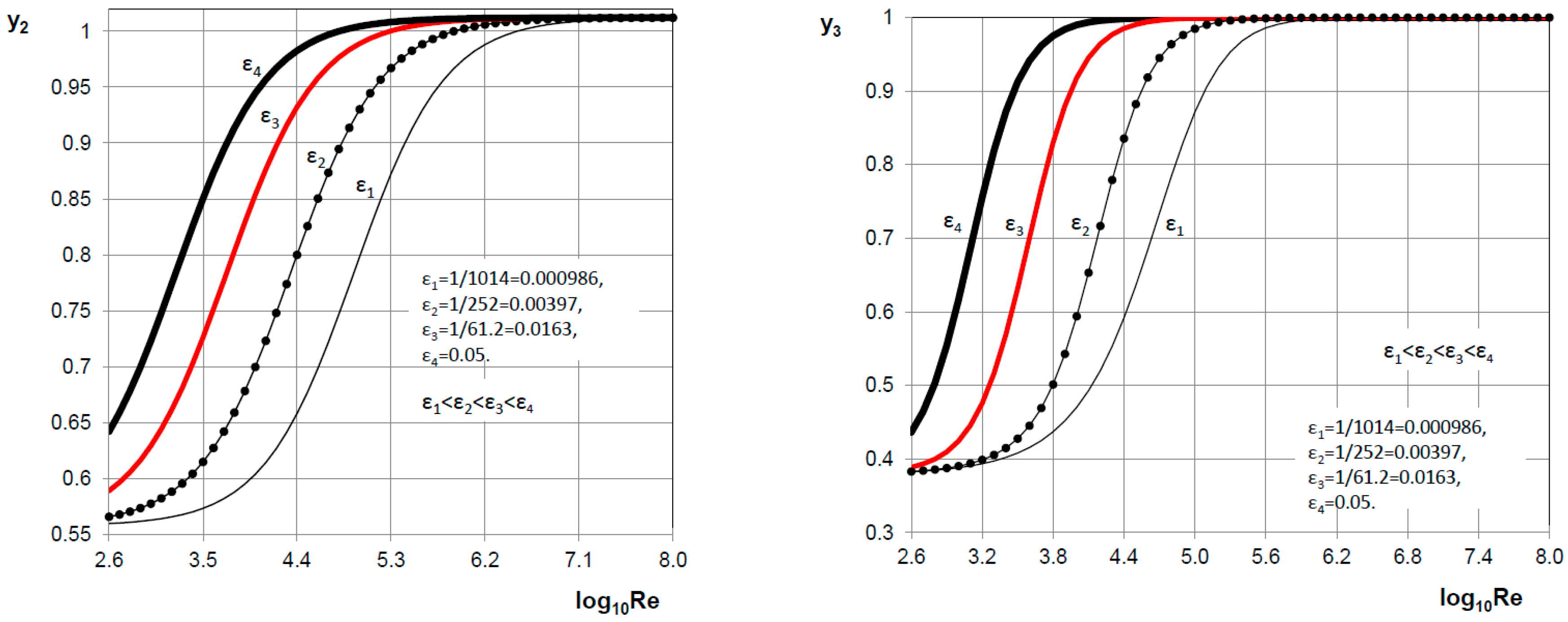
Figure 5.
Switching function as a function of the Reynolds number, with the main purpose of providing a transition between laminar flow and smooth turbulent flow .
Figure 5.
Switching function as a function of the Reynolds number, with the main purpose of providing a transition between laminar flow and smooth turbulent flow .

Figure 6.
Switching functions and with the main purpose of providing a transition between smooth turbulent flow and fully developed rough turbulent flow .
Figure 6.
Switching functions and with the main purpose of providing a transition between smooth turbulent flow and fully developed rough turbulent flow .

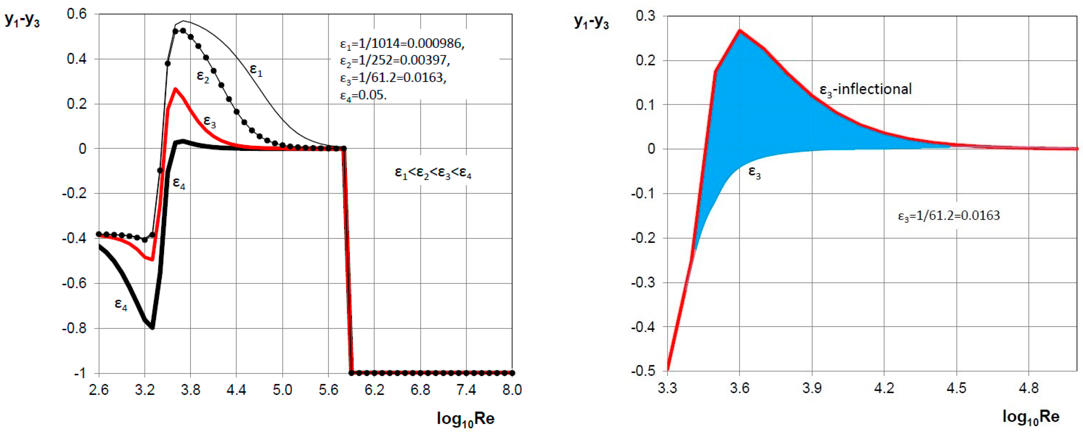
Figure 7.
Functions with the main purpose of providing Nikuradse’s inflectional shape of flow friction curves. The right side consists of a magnified detail from the left side; the blue area represents the difference between the Colebrook–White monotonic and the Nikuradse inflectional shapes.
Figure 7.
Functions with the main purpose of providing Nikuradse’s inflectional shape of flow friction curves. The right side consists of a magnified detail from the left side; the blue area represents the difference between the Colebrook–White monotonic and the Nikuradse inflectional shapes.

Figure 8.
A comparison of some correlations for the hydraulically smooth turbulent regime.

Figure 9.
The unified hydraulic model I; Equation (15).

Figure 10.
The unified hydraulic model II; Equation (15).


Table 1.
Power-law relations for the hydraulically smooth turbulent regime.
| Equation in Form: λ = A·Re−B | Coefficient A | Exponent B |
|---|---|---|
| Renouard | 0.172 | 0.18 |
| 1/10 power law | 0.139 | 0.18 |
| modified 1/9 power law | 0.184 | 0.2 |
| 1/9 power law | 0.1748 | 0.2 |
| 1/8 power law | 0.2252 | 0.22 |
| 1/7 power law | 0.3052 | 0.25 |
| Müller | 0.3564 | 0.26 |
| Blasius | 0.3164 | 0.25 |
| Panhandle A | 0.08475 | 0.1461 |
| Panhandle B | 0.01471 | 0.03922 |
| IGT (Institute of Gas Technology) | 0.18086 | 0.19726 |
| Towler and Pope | 0.09458 | 0.15174 |
| Mokhatab | 0.02 | 0.185 |
| Hodanovič | 0.22 | 0.185 |
© 2018 by the authors. Licensee MDPI, Basel, Switzerland. This article is an open access article distributed under the terms and conditions of the Creative Commons Attribution (CC BY) license (http://creativecommons.org/licenses/by/4.0/).
Share and Cite
MDPI and ACS Style
Brkić, D.; Praks, P. Unified Friction Formulation from Laminar to Fully Rough Turbulent Flow. Appl. Sci. 2018, 8, 2036. https://0-doi-org.brum.beds.ac.uk/10.3390/app8112036
AMA Style
Brkić D, Praks P. Unified Friction Formulation from Laminar to Fully Rough Turbulent Flow. Applied Sciences. 2018; 8(11):2036. https://0-doi-org.brum.beds.ac.uk/10.3390/app8112036
Chicago/Turabian StyleBrkić, Dejan, and Pavel Praks. 2018. "Unified Friction Formulation from Laminar to Fully Rough Turbulent Flow" Applied Sciences 8, no. 11: 2036. https://0-doi-org.brum.beds.ac.uk/10.3390/app8112036
Note that from the first issue of 2016, this journal uses article numbers instead of page numbers. See further details here.