Characterization of Asphalt Mixes Behaviour from Dynamic Tests and Comparison with Conventional Cyclic Tension–Compression Tests

Featured Application

Dynamic tests can be used to characterize asphalt mixes and the results obtained from dynamic tests are in good agreement with the results of conventional cyclic tests.

Abstract

In the presented research, conventional cyclic tension–compression tests and dynamic tests were performed on two types of asphalt mixes (AM). For the tension–compression tests, the complex modulus was obtained from the measurements of the axial stress and axial strain. For the dynamic tests, an automated impact hammer equipped with a load cell and an accelerometer were used to obtain the frequency response functions (FRFs) of the specimens at different temperatures. Two methods were proposed to back-calculate the complex modulus from the FRFs at each temperature: one using the 2S2P1D (two springs, two parabolic elements and one dashpot) model and the other considering a constant complex modulus. Then, a 2S2P1D linear viscoelastic model was calibrated to simulate the global linear viscoelastic behaviour back calculated from each of the proposed methods of analysis for the dynamic tests, and obtained from the tension–compression test results. The two methods of analysis of dynamic tests gave similar results. Calibrations from the tension–compression and dynamic tests also show an overall good agreement. However, the dynamic tests back analysis gave a slightly higher value of the norm of the complex modulus and a lower value of the phase angle compared to the tension–compression test data. This result may be explained by the nonlinearity of AM (strain amplitude is at least 100 times smaller for dynamic tests) and/or by ageing of the materials during the period between the tension–compression and the dynamic tests.

1. Introduction

Asphalt mixes (AM) have a linear viscoelastic (LVE) behaviour in the small strain domain [1] Cyclic tension–compression tests are traditionally used to determine the LVE properties of AM that are strongly dependent on frequency and temperature. However, these tests require expensive experimental devices such as hydraulic presses and are not applicable in situ. An economical alternative is to use non-destructive dynamic tests that are simple to perform and possibly adaptable for measurements on pavement structures. Impulse techniques using impact loadings [2,3] are known to provide accurate characterization of material properties in the case of elastic materials [4,5]. In the case of LVE materials, dynamic tests could be a great alternative to conventional cyclic tension–compression tests. Dynamic tests using wave propagation and measurement of the flying time [6,7,8] have been applied to LVE materials. Resonance testing considering only the fundamental resonance frequency [9,10,11] or resonant acoustic spectroscopy (RAS) [12,13,14,15] have also been applied to AM but it is not possible to describe accurately the frequency dependency behaviour of AM with these different tests. Recently, measurement of frequency response functions (FRFs) have been performed on LVE materials [16,17] and more specifically on AM [18,19,20,21]. Gudmarsson et al. [19,20] and Carret et al. [21] showed that using FRFs measurements to derive the LVE properties of AM is a very promising approach. However, characterizing accurately the LVE behaviour of AM from FRFs is not possible through a simplified analysis [22] and it requires an elaborate approach. In this paper, two different methods using finite element calculations are proposed to obtain the LVE behaviour from FRFs. The first method consists in an optimization of the continuous spectrum 2S2P1D (two springs, two parabolic elements and one dashpot) model constants to back-calculate the complex modulus at each tested temperature while the second method is a more direct back-calculation of the complex modulus at the first resonance frequency. The two methods were applied to two different types of AM representing five specimens that were tested with cyclic tension–compression tests and with dynamic tests. Experimental complex modulus values obtained from tension–compression tests and back-calculated from FRFs with the two proposed methods were used to fit the 2S2P1D model and the Williams-Landel-Ferry (WLF) constants simulating the global LVE behaviour of the material in each case. First, the materials tested in this study are presented. Then, the LVE behaviour characterization with cyclic tests and the modelling with the 2S2P1D model are introduced. Next, dynamic tests are introduced and the two proposed back-analysis methods are explained. Finally, data from tension–compression tests are compared with results from the two methods of back-analysis of the dynamic tests.

2. Materials and Methods

Two different types of AM are considered in this paper. The first material is a warm mix that was fabricated in laboratory using bitumen foam and labelled WF for warm foam. It contains 70% of reclaimed asphalt pavement (RAP) after one cycle of recycling. This material was used in a project from the French national research agency called IMPROVMURE [23]. Three specimens of this material were tested with tension–compression and dynamic tests. The second material is a mix with an optimized granular skeleton also fabricated in laboratory and labelled GB5. It contains 30% of RAP and the bitumen used is a polymer modified bitumen (PMB). Two specimens of this material were tested with tension–compression tests and dynamic tests.

Table 1. Specimens used in this study.

Specimen	Mass (g)	Height (mm)	Diameter (mm)	Density (kg/m3)	Void Ratio (%)	Bitumen Content (%)	RAP Content (%)
WF-4	1293	0.123	75	2379	6.6	5.4	70
WF-6	1320	0.123	75	2431	4.2	5.4	70
WF-8	1330	0.123	75	2449	3.8	5.4	70
GB5-3	941	0.152	64	2381	4.8	4.8	30
GB5-4	951	0.152	64	2378	5.1	4.8	30

gives some indications on the five studied specimens. The tension–compression tests were performed first and the dimensions listed in Table 1 correspond to the dimensions after the specimens were cut (see Section 3.1) before performing the dynamic tests.

3. Characterization of the Linear Viscoelastic (LVE) Behaviour

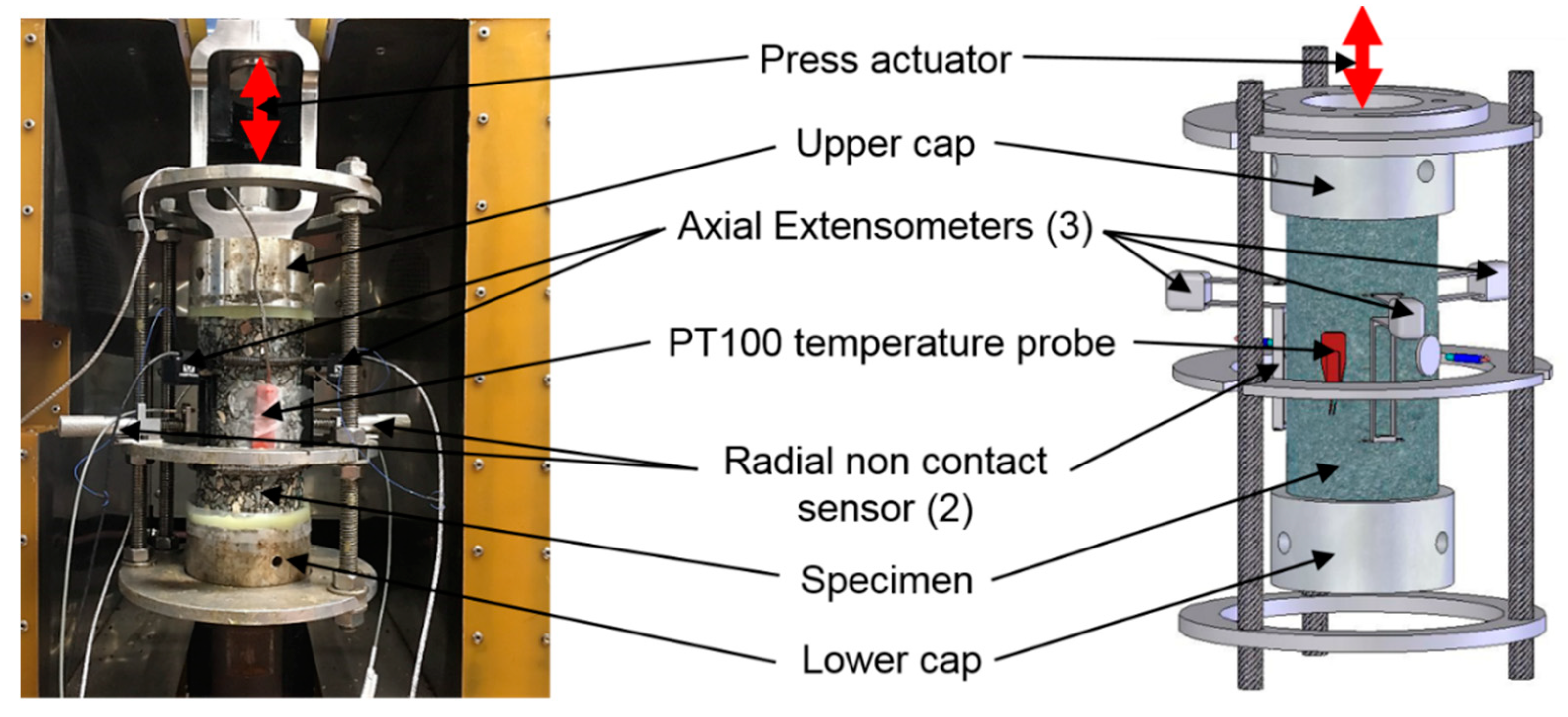
3.1. Cyclic Tension–Compression Tests

Cyclic tension–compression tests were first performed to determine the complex modulus and complex Poisson’s ratio of the five considered cylindrical specimens. A hydraulic press was used in strain-controlled mode to apply cyclic sinusoidal axial loadings with an amplitude of around 50 μm/m. The axial stress σ_z was measured with a load cell, the axial strain ε_z was obtained from the average of three extensometers placed at 120° from each other, and the radial strain ε_r was derived from the measurements of two non-contact sensors. The procedure developed at ENTPE/University of Lyon laboratory is detailed in other publications [24,25,26]. The complex notation of the axial stress, the axial strain and the radial strain are given in Equation (1):

$$\begin{array}{l}{\mathsf{\sigma }}_{\mathrm{z}}^{*}={\mathsf{\sigma }}_{0\mathrm{z}}·{\mathrm{e}}^{\mathrm{j}\mathsf{\omega }\mathrm{t}}\\ {\mathsf{\epsilon }}_{\mathrm{z}}^{*}={\mathsf{\epsilon }}_{0\mathrm{z}}·{\mathrm{e}}^{\mathrm{j}(\mathsf{\omega }\mathrm{t}+{\mathsf{\phi }}_{\mathsf{\epsilon }\mathrm{z}})}\\ {\mathsf{\epsilon }}_{\mathrm{r}}^{*}={\mathsf{\epsilon }}_{0\mathrm{r}}·{\mathrm{e}}^{\mathrm{j}(\mathsf{\omega }\mathrm{t}+{\mathsf{\phi }}_{\mathsf{\epsilon }\mathrm{r}})}\end{array}$$

(1)

where ω is the pulsation (ω = 2πf, where f is the frequency), σ_0z is the norm of the complex axial stress and ε_0z and ϕ_εz (respectively, ε_0r and ϕ_εr) are the norm and phase angle of the complex axial strain (respectively, complex radial strain). The tension–compression tests were performed at eight loading frequencies (0.003, 0.01, 0.03, 0.1, 0.3, 1, 3 and 10 Hz) and nine temperatures from −25 °C to 55 °C in steps of 10 °C. Details of the experimental set up are shown in Figure 1. The complex modulus (respectively, complex Poisson’s ratio) are defined as the ratio between the axial stress and the axial strain (respectively, the opposite of the radial strain and the axial strain) and they are calculated at each temperature and frequency as follow:

$${\mathrm{E}}^{*}=\frac{{\mathsf{\sigma }}_{\mathrm{z}}^{*}}{{\mathsf{\epsilon }}_{\mathrm{z}}^{*}}=\left|{\mathrm{E}}^{*}\right|·{\mathrm{e}}^{\mathrm{j}{\mathsf{\phi }}_{\mathrm{E}}}$$

(2)

$${\mathsf{\nu }}^{*}=-\frac{{\mathsf{\epsilon }}_{\mathrm{r}}^{*}}{{\mathsf{\epsilon }}_{\mathrm{z}}^{*}}=\left|{\mathsf{\nu }}^{*}\right|·{\mathrm{e}}^{\mathrm{j}{\mathsf{\phi }}_{\mathsf{\nu }}}$$

(3)

where E* is the complex modulus, ϕ_E is the phase angle of the complex modulus, ν* is the complex Poisson’s ratio and ϕ_ν is the phase angle of the complex Poisson’s ratio.

3.2. Modelling of the LVE Behaviour: 2S2P1D Rheological Model

The continuous spectrum 2S2P1D model developed at ENTPE [27,28,29] was used to model the LVE behaviour of AM. This model is the association in series of two springs, two parabolic creep elements and one dashpot. In the three-dimension case [30], the expressions of the complex modulus and the complex Poisson’s ratio, for isotropic behaviour, are given at a given reference temperature (Tref), by Equations (4) and (5), respectively.

$${\mathrm{E}}_{2\mathrm{S}2\mathrm{P}1\mathrm{D}}^{*}(\mathsf{\omega })={\mathrm{E}}_{00}+\frac{{\mathrm{E}}_0-{\mathrm{E}}_{00}}{1+\mathsf{\delta }{(\mathrm{j}\mathsf{\omega }{\mathsf{\tau }}_{\mathrm{E}})}^{-\mathrm{k}}+{(\mathrm{j}\mathsf{\omega }{\mathsf{\tau }}_{\mathrm{E}})}^{-\mathrm{h}}+{(\mathrm{j}\mathsf{\omega }\mathsf{\beta }{\mathsf{\tau }}_{\mathrm{E}})}^{-1}}$$

(4)

$${\mathsf{\nu }}_{2\mathrm{S}2\mathrm{P}1\mathrm{D}}^{*}(\mathsf{\omega })={\mathsf{\nu }}_{00}+\frac{{\mathsf{\nu }}_0-{\mathsf{\nu }}_{00}}{1+\mathsf{\delta }{(\mathrm{j}\mathsf{\omega }{\mathsf{\tau }}_{\mathsf{\nu }})}^{-\mathrm{k}}+{(\mathrm{j}\mathsf{\omega }{\mathsf{\tau }}_{\mathsf{\nu }})}^{-\mathrm{h}}+{(\mathrm{j}\mathsf{\omega }\mathsf{\beta }{\mathsf{\tau }}_{\mathsf{\nu }})}^{-1}}$$

(5)

where ω is the pulsation (ω = 2πf, where f is the frequency), E₀ and ν₀ are the high frequency modulus and Poisson’s ratio, E₀₀ and ν₀₀ are the low frequency modulus and Poisson’s ratio, k and h are dimensionless constants such as 0 < k < h < 1, δ is a dimensionless constant, and β is a dimensionless constant related to Newtonian viscosity η by η = (E₀ − E₀₀) βτ_E. τ_E and τ_ν are characteristic time constants of the complex modulus and Poisson’s ratio linked by a constant ratio. The values of the characteristic times vary only with temperature. The time temperature superposition principle (TTSP) is verified for asphalt mixes in the linear and nonlinear domains [31,32,33] so it is possible to calculate the characteristic time at any given temperature using Equation (6):

$$\mathsf{\tau }(\mathrm{T})={\mathrm{a}}_{\mathrm{T}}(\mathrm{T}){\mathsf{\tau }}_{\mathrm{ref}}$$

(6)

where τ_ref is the characteristic time at the reference temperature (τ_E or τ_ν) and a_T is the shift factor at the temperature T defined by the Williams–Landel–Ferry (WLF) equation [34]:

$$\log ({\mathrm{a}}_{\mathrm{T}})=-\frac{{\mathrm{C}}_1(\mathrm{T}-{\mathrm{T}}_{\mathrm{ref}})}{{\mathrm{C}}_2+\mathrm{T}-{\mathrm{T}}_{\mathrm{ref}}}$$

(7)

where C₁ and C₂ are the two constants of the WLF equation and T_ref is the reference temperature.

4. Dynamic Tests

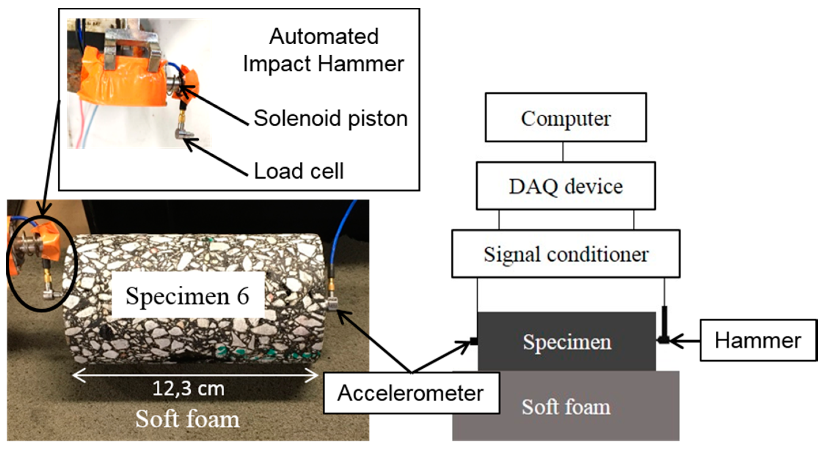
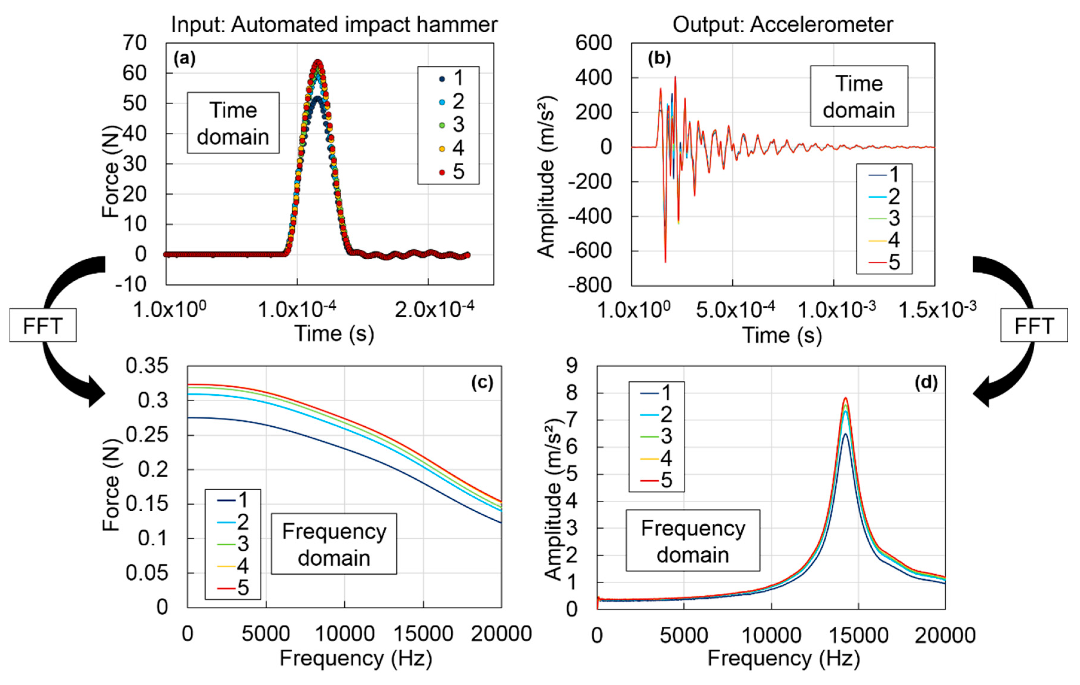
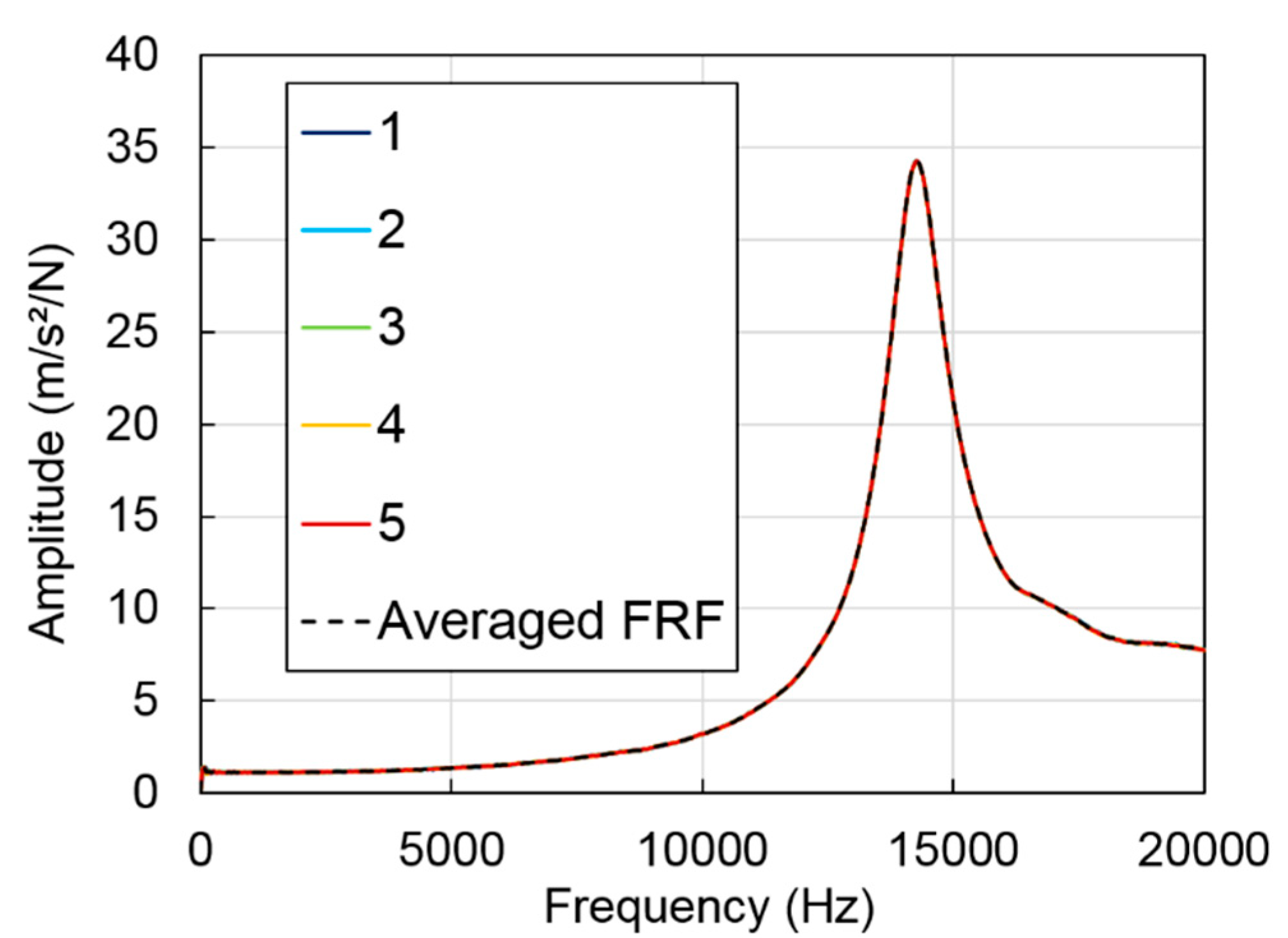
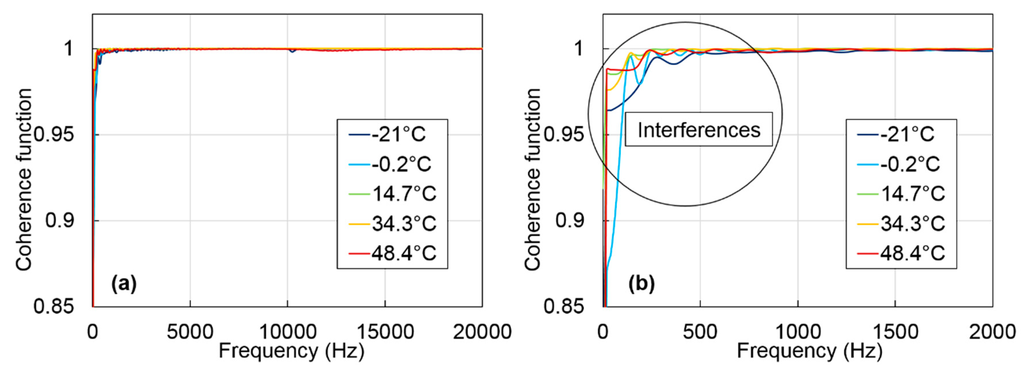
4.1. Measurement of the Frequency Response Functions (FRFs)

First, the specimens used for complex modulus tension–compression test were sawed to separate the glued upper and lower metallic caps before performing the dynamic measurements. An impact hammer equipped with a load cell (PCB model 086E80) was used as an external source of excitation. The order of magnitude of the maximum strain induced in the specimen by the impact is of about 0.1 μm/m [18,21]. The impact hammer was automated with a solenoid piston programmed with a microcontroller (Arduino Uno R3) to improve the repeatability of the test and to allow measurements directly inside a thermal chamber. This automated system was inspired by systems previously developed by Norman et al. in 2012 and Brüggemann et al. in 2015 [35,36]. The response of the materials was recorded with an accelerometer (PCB model 353B15). The impact hammer and the accelerometer were connected to a signal conditioner (PCB model 482C15) and the signal conditioner was connected to a data acquisition device (NI USB-6356) connected to a computer. To achieve free boundary conditions, soft foam was placed under the specimens during the tests. In this study, only the longitudinal compression mode of vibrations was considered. For this mode of vibrations, the impact is applied in the centre of one short side of the cylinder while the acceleration is measured in the centre of the opposite short side. The experimental set up for the dynamic tests corresponding to the longitudinal mode of vibrations is presented in Figure 2.

The measurements were recorded with a sampling frequency of 1 MHz by using a MATLAB application which was specifically developed for this test. Measurements were performed at five temperatures (−20, 0, 15, 35 and 50 °C) and five impacts were applied at each temperature. The applied force and the acceleration were recorded for each impact. The experimental data in time domain were then converted in frequency domain with a 1 Hz resolution using the Fast Fourier Transform (FFT). Figure 3 shows an example of the signals in time and frequency domains for specimen GB5-3 at 14.7 °C (measured temperature with a probe at the surface of the specimen).

As shown in Figure 3, the frequency spectrum of the impact contains energy up to 20 kHz, which is the maximum frequency considered for the calculations of frequency response functions (FRFs) in this study. FRFs were calculated from the frequency domain signals as follow:

$$\mathrm{H}(\mathrm{f})=\left(\overline{\mathrm{Y}(\mathrm{f})·\mathrm{X}*(\mathrm{f})}\right)/\left(\overline{\mathrm{X}(\mathrm{f})·\mathrm{X}*(\mathrm{f})}\right)$$

(8)

where H is the FRF, Y is the FFT of the measured acceleration, X is the FFT of the applied force, X* is the complex conjugate of the applied force and the bar above corresponds to the arithmetic average from the five impacts. The five FRFs corresponding to each of the five impacts and the averaged FRF (Equation (8)) for specimen GB5-3 at 14.7 °C are displayed on Figure 4. Figure 4 shows that the six FRFs overlaps, which confirms the very good repeatability of the test.

Quality of the measurements was also checked with the coherence function. The coherence is a value between 0 and 1 that indicates how much of the vibratory response recorded with the accelerometer is due to the impact. For a value of 1, the response is fully explained by the impact while decreasing values indicate that something has disrupted the test. Coherence function is calculated according to Equation (9):

$$\mathrm{C}\mathrm{F}(\mathrm{f})={\left(\overline{\mathrm{X}*(\mathrm{f})·\mathrm{Y}(f)}\right)}^2/\left(\left(\overline{\mathrm{X}(\mathrm{f})·\mathrm{X}*(\mathrm{f})}\right)·\left(\overline{\mathrm{Y}(\mathrm{f})·\mathrm{Y}*(\mathrm{f})}\right)\right)$$

(9)

where CF is the coherence function, Y and Y* are the FFT of the measured acceleration and its complex conjugate, X and X* are the FFT of the applied force and its complex conjugate and the bar above corresponds to the arithmetic average. The coherence functions of specimen GB5-3 for the five tested temperatures are presented in Figure 5. For all temperatures, the coherence function is very good with values close to one for frequencies higher than 1000 Hz. It is therefore recommended to not use the frequencies below 1000 Hz.

4.2. Calculation of FRFs with the Finite Element Method (FEM)

Numerical FRFs were calculated with the finite element method (FEM) considering linear viscoelastic behaviour and the dynamic test boundary conditions. Figure 6 shows the FEM mesh and boundary conditions used for the FEM calculation of the FRFS.

FRFs were calculated at the desired frequencies by resolving the following three-dimensional equation of motion in frequency domain:

$$-\mathsf{\rho }{\mathsf{\omega }}^2\mathbf{u}-\nabla ·\mathsf{\sigma }=0$$

(10)

where ρ is the bulk density of the material, ω is the angular frequency, u is the displacement vector, ∇ is the gradient tensor operator and σ is the Cauchy stress tensor. Free boundary conditions are assumed to solve Equation (10) except at the impact point where a cyclic load e^iωt is applied in the direction of the impact. Since the load amplitude is unity, the calculated FRFs correspond to the calculated acceleration in direction Z (direction of vibration of the accelerometer in physical tests). Back analysis was performed considering two LVE behaviour models successively, as explained below.

4.3. Determination of the Material LVE Properties from Dynamic Tests

The LVE properties of the material were determined from the FRFs measured with the dynamic tests in two steps. The first step is a back-calculation of the complex modulus of the material at each tested temperature. Two methods, presented in the next sections, were used for this purpose. They consist in optimizing the constants of the LVE model used to calculate FRFs so that calculated FRFs match the experimental measured FRFs using dynamic tests at the considered temperature. The second step, which is the same for the two proposed methods, consists in using the complex modulus values determined in the first step at each temperature to fit a 2S2P1D model and a WLF law simulating the global LVE behaviour of the material. This operation is similar to what is done with the tension–compression test data.

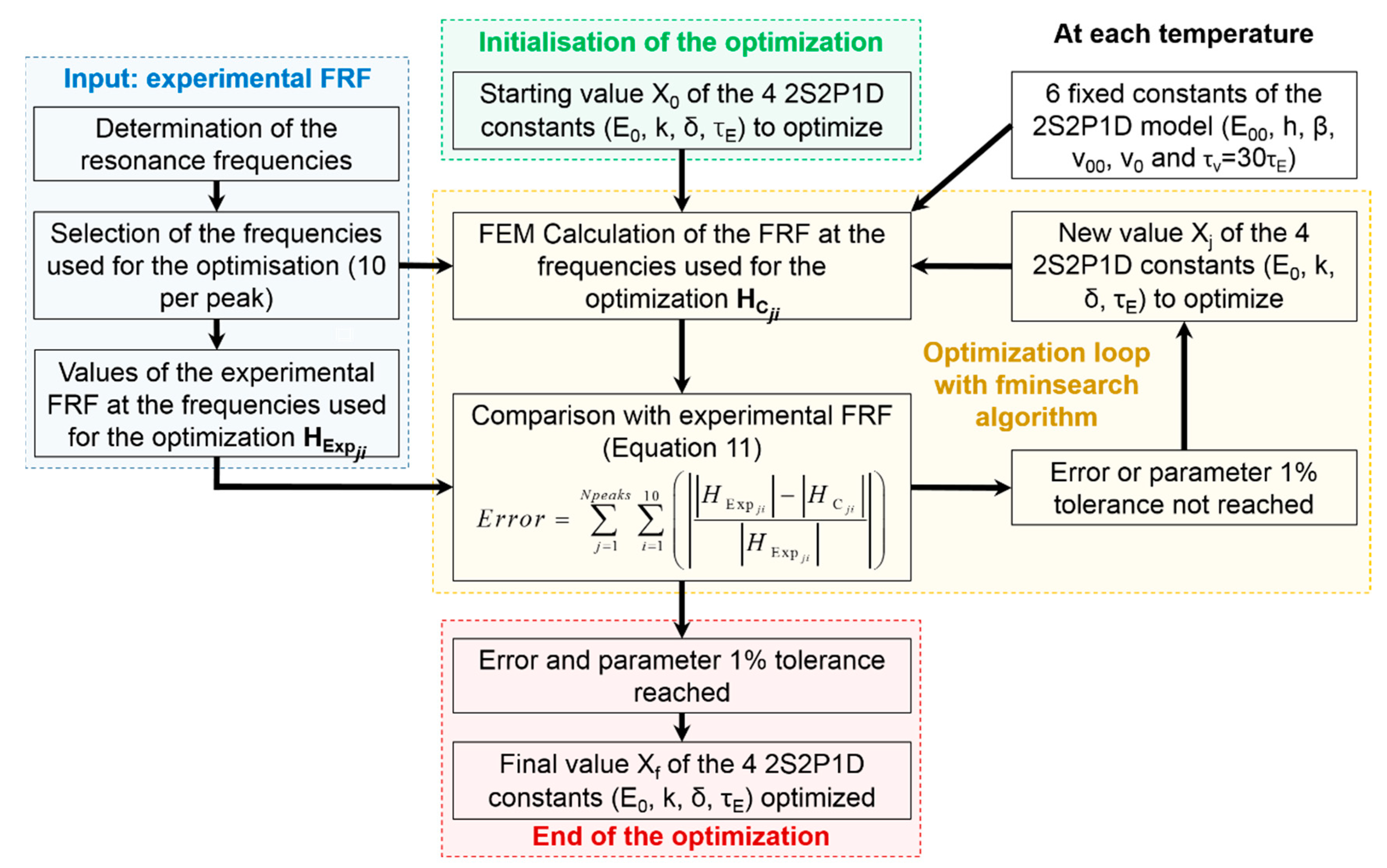
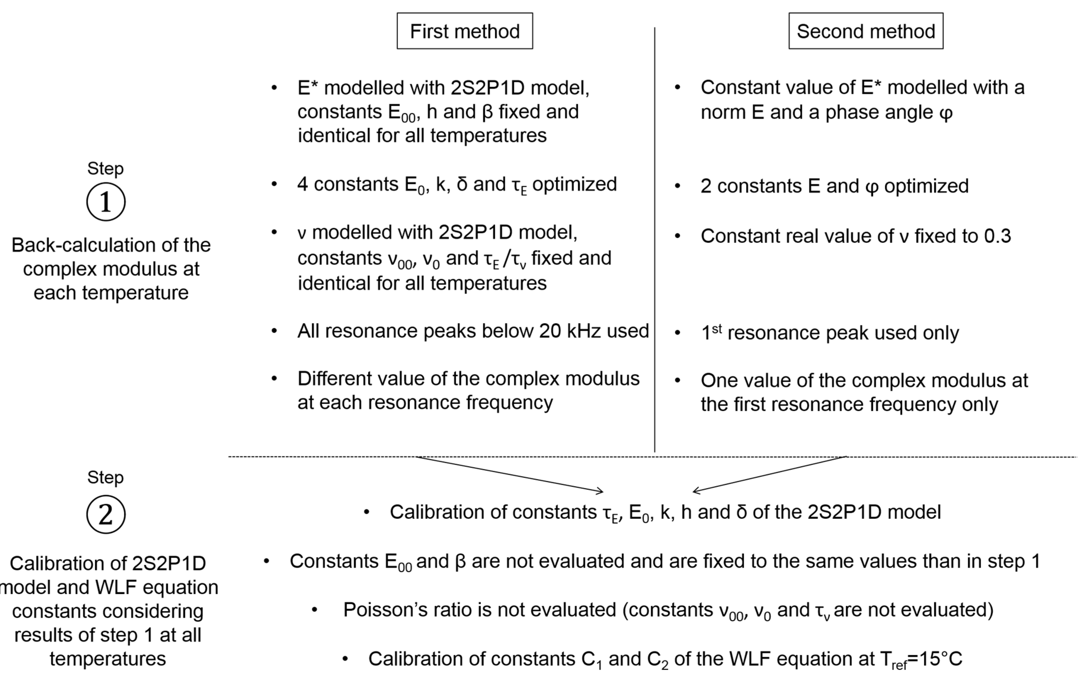
4.3.1. First Method: Optimization of the 2S2P1D Model Constants to Match Experimental FRFs

Among the 10 constants of the 2S2P1D model, only four constants (E₀, k, δ and τ_E) have a significant influence for the considered range of frequencies involved during dynamic tests and need to be optimized. The complex Poisson’s ratio has a very small influence on the calculation of the FRFs below 20 kHz. Poisson’s ratio cannot be back-calculated with this procedure; however, it is necessary to assume values for constants ν₀₀, ν₀ and τ_ν to back-calculate the complex modulus at each temperature. For each tested temperature, the vector X of the four constants (E₀, k, δ and τ_E) to be identified was optimized iteratively so that the calculated FRFs match the experimental FRFs. The values of the six other constants were fixed to classical values for AM: E₀₀ = 100 MPa, ν₀ = 0.19, ν₀₀ = 0.45, h = 0.53, β = 250 and τ_ν = 31.6τ_E. Only the values of the experimental FRFs at frequencies around the resonance frequencies are used as input in the optimization according to previous studies [19,20,21] that showed their meaningful importance. Ten frequencies were selected along each resonance peak and the error function to minimize was defined as follow:

$$\mathrm{Error}={\displaystyle \sum _{\mathrm{j}=1}^{\mathrm{Npeaks}}{\displaystyle \sum _{\mathrm{i}=1}^{10}\left(\left|\frac{\left|{\mathrm{H}}_{{\mathrm{Exp}}_{\mathrm{ji}}}\right|-\left|{\mathrm{H}}_{{\mathrm{C}}_{\mathrm{ji}}}\right|}{\left|{\mathrm{H}}_{{\mathrm{Exp}}_{\mathrm{ji}}}\right|}\right|\right)}}$$

(11)

where H_Exp is the experimental FRF, H_C is the calculated FRF, N_peaks is the number of resonance peaks, j is the index of the peak and i is the index of the frequencies. The number of peaks considered for the optimization at each temperature corresponds to the number of peaks that are visible below 20 kHz (maximum considered frequency with our experimental device). This number is given in

Table 2. Number of peaks considered for the optimization of the 2S2P1D model constants at each temperature.

Temperature (°C)	−20	0	15	35	50
Number of peaks	1	1	1	1	2

for each temperature.

The optimization was performed in MATLAB with the “fminsearch” algorithm and the optimization was stopped when the error and the parameter tolerance of 1% is reached (e.g., when the variation of the error and of all the values of the four constants to be identified is less than 1% between two iterations of the algorithm). The final vector X_f of the four constants (E₀, k, δ and τ_E) was then used with the three fixed constants related to the complex modulus (E₀₀, h, and β) to back-calculate the complex modulus at the resonance frequencies of the peaks used as input for the optimization at the considered temperature. The optimization procedure to identify the four 2S2P1D model constants (E₀, k, δ and τ_E) at each temperature is explained in Figure 7.

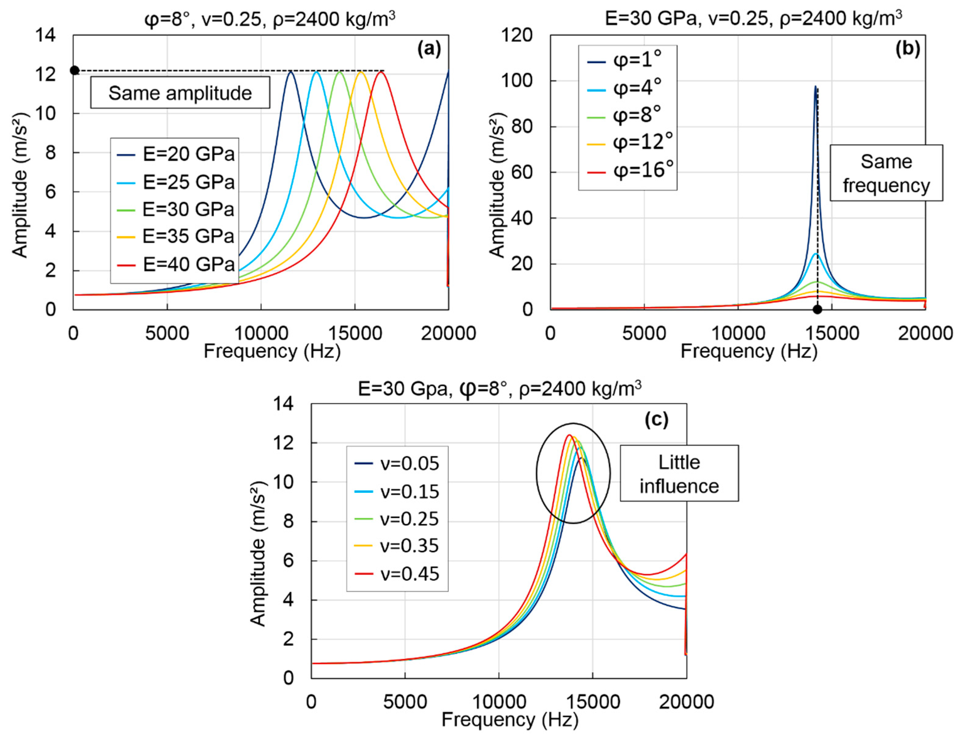
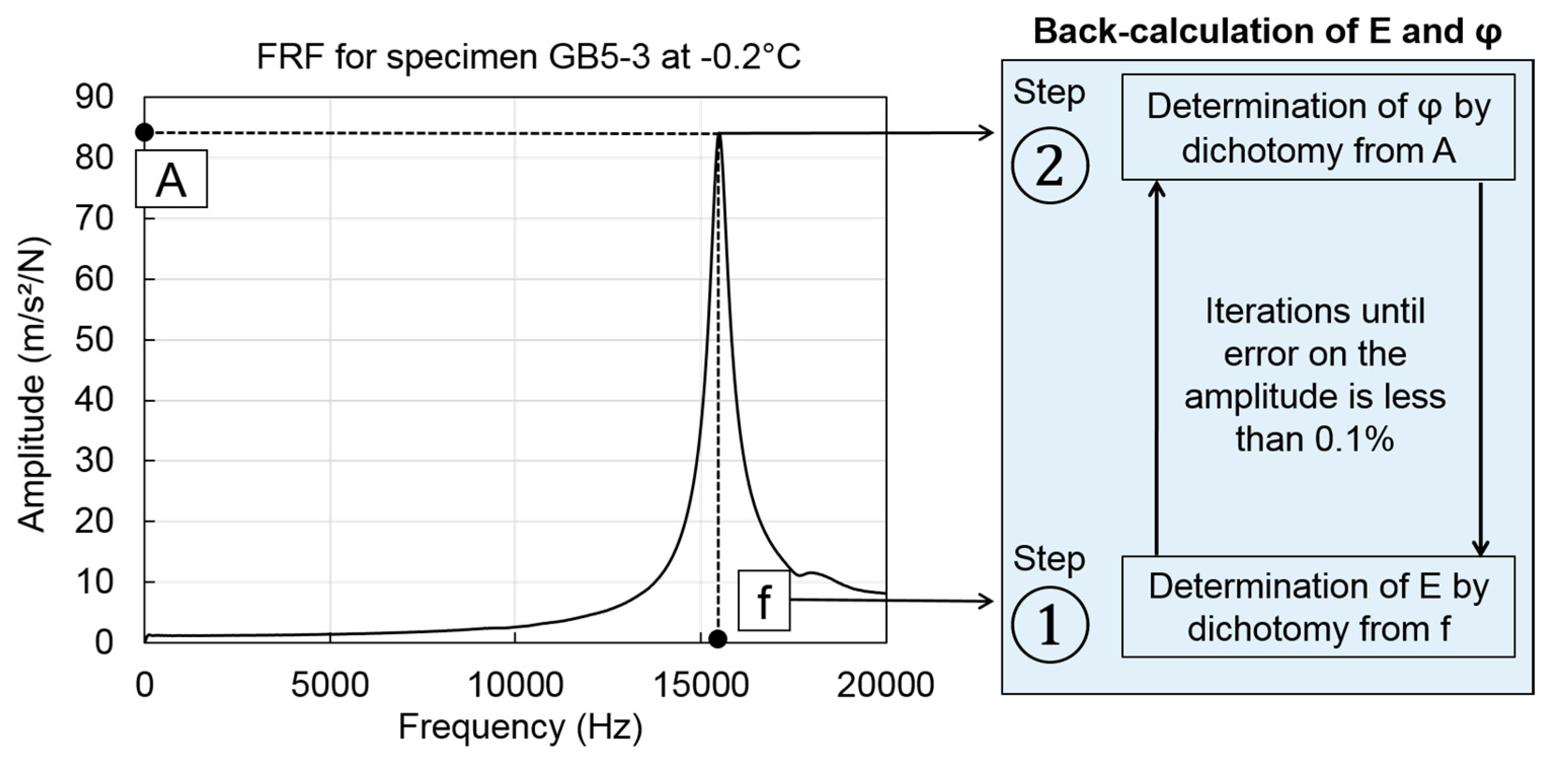
4.3.2. Second Method: Constant Complex Modulus Obtained from the First Resonance Peak Only

The second method is a simplified approach that does not require, in the first step, a rheological LVE model considering the frequency and temperature dependence. At each tested temperature, a constant complex modulus value and a constant real Poisson’s ratio of 0.3 were considered. A numerical sensitivity analysis was performed to evaluate the influence of the norm and phase angle of the complex modulus and the real value of the Poisson’s ratio on the calculation of FRFs. The influence of each LVE constant was evaluated from FRFs calculated for five values taken in the range of variation of the considered LVE constant while the two others are fixed. Table 2 lists the five values considered for each LVE constant and the corresponding fixed values of the two others. Some results are shown on Figure 8 for a cylinder with similar dimensions than those used in this study and with a density of 2400 kg/m³. It is shown in Figure 8 that the norm of the complex modulus has an important influence on the first resonance frequency but not on the amplitude. It is the reverse for the phase of the complex modulus, while Poisson’s ratio has little influence on both the frequency and the amplitude.

To confirm the observation raised in Figure 8, the relative standard deviations (RSD) for the first resonance frequency and amplitude were calculated for the three studied constants. Results are given in

Table 3. Influence of E, ϕ and ν on the first resonance frequency and FRF amplitude. When one of the constants varies, the two other constants are fixed at the values listed in the left column.

	E (GPa)	20	25	30	35	40	RSD (%)
ϕ = 8°	f (Hz)	11,580	12,940	14,180	15,320	16,380	13.5
ν = 0.25	Amplitude (m/s²)	12.1	12.1	12.1	12.1	12.1	6 × 10−4
	ϕ (°)	1	4	8	12	16	RSD (%)
E = 30 GPa	f (Hz)	14,120	14,140	14,180	14,240	14,340	0.6
ν = 0.25	Amplitude (m/s²)	97.7	24.4	12.1	8.0	5.9	130.8
	ν	0.05	0.15	0.25	0.35	0.45	RSD (%)
E = 30 GPa	f (Hz)	14,400	14,320	14,180	13,980	13,760	1.8
ϕ = 8°	Amplitude (m/s²)	11.2	11.8	12.1	12.3	12.4	4.0

. They confirm the previous observations and also indicate that the norm of the complex modulus has really no impact on the peak amplitude while the phase has a very little influence on the frequency. The Influence of the Poisson’s ratio can be considered as negligible when compared with the influence of the two other constants. Observations presented in Figure 8 and Table 3 justify the assumption of a constant real value of 0.3 for the Poisson’s ratio. In addition, the identification of the norm and phase of the complex modulus can be separated into two steps: the norm can be determined by dichotomy from the first resonance frequency and then the phase can be determined by dichotomy from the corresponding amplitude. This process was repeated iteratively until the error on the amplitude is less than 0.1%. Figure 9 shows the principle of the back-calculation of the complex modulus using the first resonance peak of the FRFs.

4.3.3. Summary and Remarks on the Two Methods

Differences between the two proposed methods concern the first step in which the complex modulus is back-calculated at each temperature, while the second step is identical for the two methods. First, the assumptions on the Poisson’s ratio value are different in the two methods. In the first method, the Poisson’s ratio is a complex number, which depends on the frequency and on the temperature, and is modelled with the 2S2P1D model assuming the values of constants ν₀₀, ν₀ and τ_E/τ_ν. In the second method, a constant real value of Poisson’s ratio equal to 0.3 is assumed. Another difference is that all resonance peaks under 20 kHz are considered in the first method while only the first resonance peak is used in the second method. Consequently, the second method gives only one value of the complex modulus at each temperature while the first method gives values for each resonance frequency. This difference is not essential in this study since 50 °C is the only temperature for which two peaks were observed. However, it can be interesting to evaluate more than one value of the complex modulus at each temperature. Finally, in the first method, four constants are evaluated at each temperature using a complex algorithm. In the second method, only two constants are evaluated using a simple dichotomy process. The second method is therefore very easy to apply and time-effective compared to the first method. Figure 10 highlights the main differences between the first step of the two methods and gives the principle of the second step that is identical for the two methods. Note that, even though the same constant h is fixed for the back-calculation at each temperature (in the first step of first method), a different constant h value can be obtained during the calibration process of the second step.

5. Results

5.1. Tension–Compression Tests Results

Results of the tension–compression tests for specimen WF-8 are plotted in Figure 11. A continuous curve can be seen on the Cole–Cole diagram, which indicates that the material is rheologically simple and that the time–temperature superposition principle (TTSP) is valid. The master curve of the norm of the complex modulus is plotted at a reference temperature (T_ref) of 15 °C in Figure 11. The 2S2P1D model was fitted to the experimental data and is also plotted in Figure 11. A very good agreement between the experimental data and the 2S2P1D model can be observed.

The values of the 2S2P1D model and WLF equation constants obtained from the tension–compression tests are given for all specimens in

Table 4. Calibrated 2S2P1D constants to match tension–compression measurements.

Specimen	E00 (MPa)	E0 (MPa)	δ	k	h	β	τE15°C (s)	C1	C2
WF-4	28	33,400	2.28	0.177	0.57	154	5.4 × 10−2	24.9	166.6
WF-6	40	37,500	2.28	0.177	0.57	154	7.0 × 10−2	24.9	166.6
WF-8	56	36,900	2.28	0.177	0.57	154	6.9 × 10−2	24.9	166.6
GB5-3	65	39,100	1.80	0.180	0.60	350	7.5 × 10−2	24.7	165.9
GB5-4	65	39,500	1.80	0.180	0.60	350	1.5 × 10−1	24.7	165.9

. The constants k, h, δ, β, C₁ and C₂ have the same values for a given material because they are only depending on the bitumen and not on the granular skeleton as shown in previous research [27,37,38].

The measurements were recorded with a sampling frequency of 1 MHz by using a MATLAB application which was specifically developed for this test. Measurements were performed at five temperatures (−20, 0, 15, 35 and 50 °C) and five impacts were applied at each temperature. The applied force and the acceleration were recorded for each impact. The experimental data in time domain were then converted in frequency domain with a 1 Hz resolution using the Fast Fourier Transform (FFT). Figure 3 shows an example of the signals in time and frequency domains for specimen GB5-3 at 14.7 °C (measured temperature with a probe at the surface of the specimen).

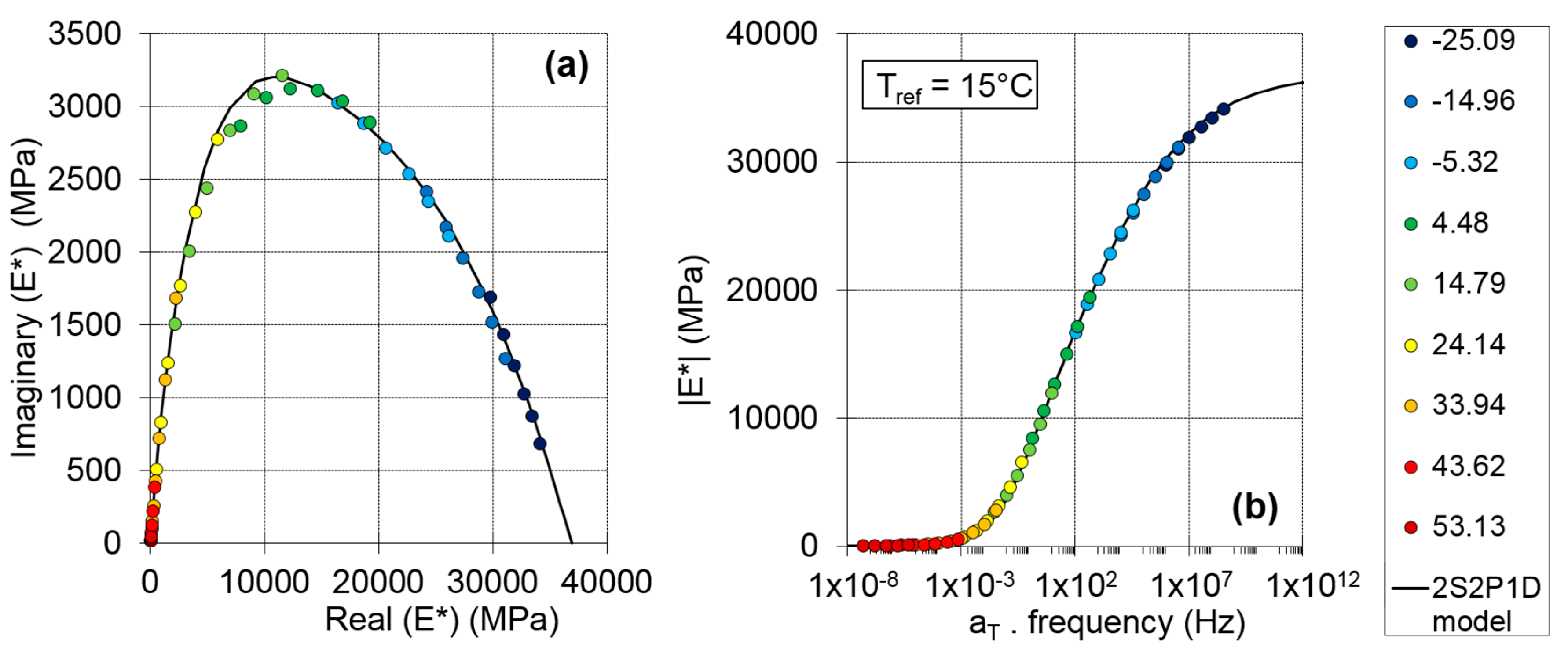
5.2. Dynamic Impact Tests Results

The complex modulus values back-calculated at each temperature from the FRFs measurements with the two proposed methods for specimen WF-8 are plotted, as an example, in Figure 12. For the first method of back-calculation, one value of the complex modulus is plotted for temperatures at which only one peak was considered for the optimization (−20, 0, 15 and 35 °C) and two values are plotted at −50 °C because two peaks exist for this temperature. Only one value of the complex modulus is presented for each temperature for Method 2 because the back-calculation is limited to the first resonance frequency, as explained previously. The master curve of the norm of the complex modulus at 15 °C was obtained considering the validity of the TTSP. The 2S2P1D model was fitted to the back-calculated modulus for both methods and the two resulting 2S2P1D model curves are also plotted in Figure 12. Good fitting of the 2S2P1D curves can be observed for both methods, which give only slightly different results.

The values of the 2S2P1D model and WLF equation constants fitting the results from the two back-analysis methods are given for all specimens in

Table 5. Calibrated 2S2P1D constants to match complex modulus back-calculated from dynamic tests with the first method using 2S2P1D model at each temperature. Constants E₀₀ and β are assumed to be 100 MPa and 250, respectively.

Specimen	E00 (MPa)	E0 (MPa)	δ	k	h	β	τE15°C (s)	C1	C2
WF-4	100	34,800	1.39	0.142	0.49	250	4.0 × 10−2	18.9	133.2
WF-6	100	38,700	1.39	0.142	0.49	250	7.0 × 10−2	18.9	133.2
WF-8	100	37,500	1.39	0.142	0.49	250	4.0 × 10−2	18.9	133.2
GB5-3	100	39,100	1.17	0.130	0.442	250	5.5 × 10−2	19.2	139.5
GB5-4	100	40,500	1.17	0.130	0.442	250	7.0 × 10−2	19.2	139.5

(first method) and

Table 6. Calibrated 2S2P1D constants to match complex modulus back-calculated from dynamic tests measurements with the second method using the first resonance peak at each temperature. Constants E₀₀ and β are assumed to be 100 MPa and 250, respectively.

Specimen	E00 (MPa)	E0 (MPa)	δ	k	h	β	τE15°C (s)	C1	C2
WF-4	100	36,100	1.39	0.142	0.49	250	4.0 × 10−2	18.9	133.2
WF-6	100	39,500	1.39	0.142	0.49	250	7.0 × 10−2	18.9	133.2
WF-8	100	38,500	1.39	0.142	0.49	250	4.0 × 10−2	18.9	133.2
GB5-3	100	39,800	1.17	0.130	0.442	250	5.5 × 10−2	19.2	139.5
GB5-4	100	41,100	1.17	0.130	0.442	250	7.0 × 10−2	19.2	139.5
GB5-4	100	40,500	1.17	0.130	0.442	250	7.0 × 10−2	19.2	139.5

(second method). Note that similarly to the results of the tension–compression tests, constants k, h, δ, β, C₁ and C₂ have the same values for a given material. In addition, the same WLF equation constants can be used for the two methods and only constant E₀ differs between the first and the second method.

It must be highlighted that values of constants E₀₀ and β are assumed because they have no influence on the complex modulus values in the frequency range involved during the dynamic tests. The constants governing the value of the Poisson’s ratio ν₀₀, ν₀ and τ_ν do not appear in Table 5 and Table 6 because the Poisson’s ratio was not evaluated from the dynamic tests but assumptions on the values of these constants were necessary to back-calculate the complex modulus at each temperature in the first step of the first method. A good proximity between the results obtained with the two methods is shown in Figure 12. The same observation was made for all specimens. To validate this visual impression, the relative difference between the norm (in %) and the phase (in °) of the 2S2P1D simulated complex modulus obtained from the two methods are plotted in Figure 13. In this figure, the relative difference is plotted against the reduced frequency at 15 °C for all specimens. It is seen that the second method considering a constant complex modulus at each temperature and a constant real Poisson’s ratio of 0.3 gives a norm slightly higher than the first method with a maximum relative difference of about 3.7%. The phase angle determined with the two methods can be considered equivalent with less than 0.03° of difference, which was expected because only constant E₀ of the 2S2P1D model differs between the first and the second method. The slight differences between the two methods may be explained by the different assumptions on the Poisson’s ratio value which is modelled with the 2S2P1D model in the first method and taken constant equal to 0.3 in the second method. However, the two proposed methods are in very good agreement. This result is interesting because the second simplified method does not require in the first step the use of an elaborate LVE model. In addition, the back-calculation process is easy to perform as the two calculated constants can be identified using dichotomy process. This new simplified approach considerably reduces the computational time and offers great potential to back-calculate the complex modulus of AM from FRFs measurements using the first resonance peak only.

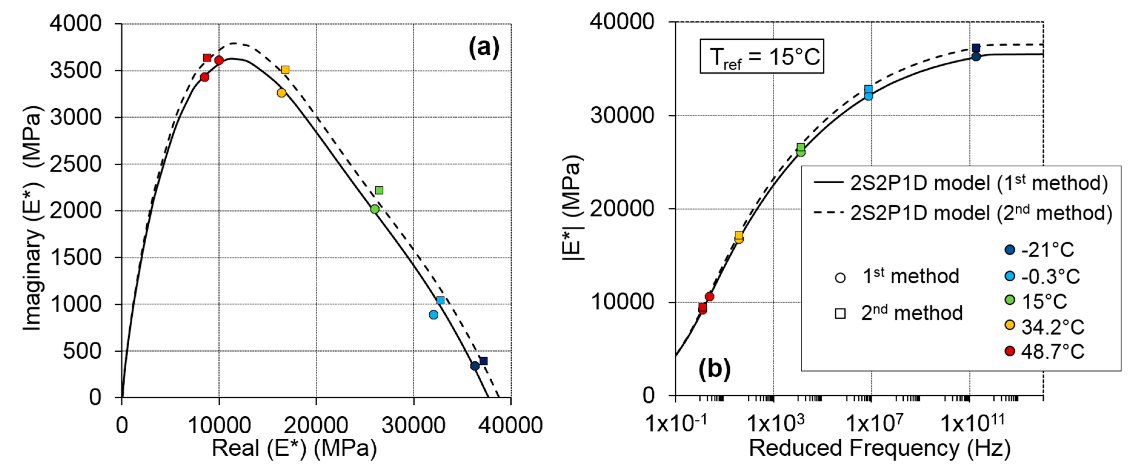
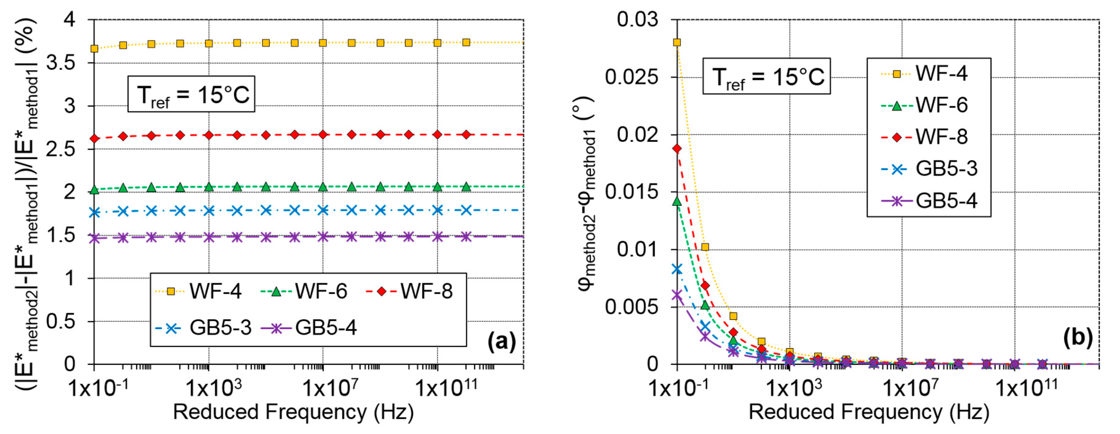
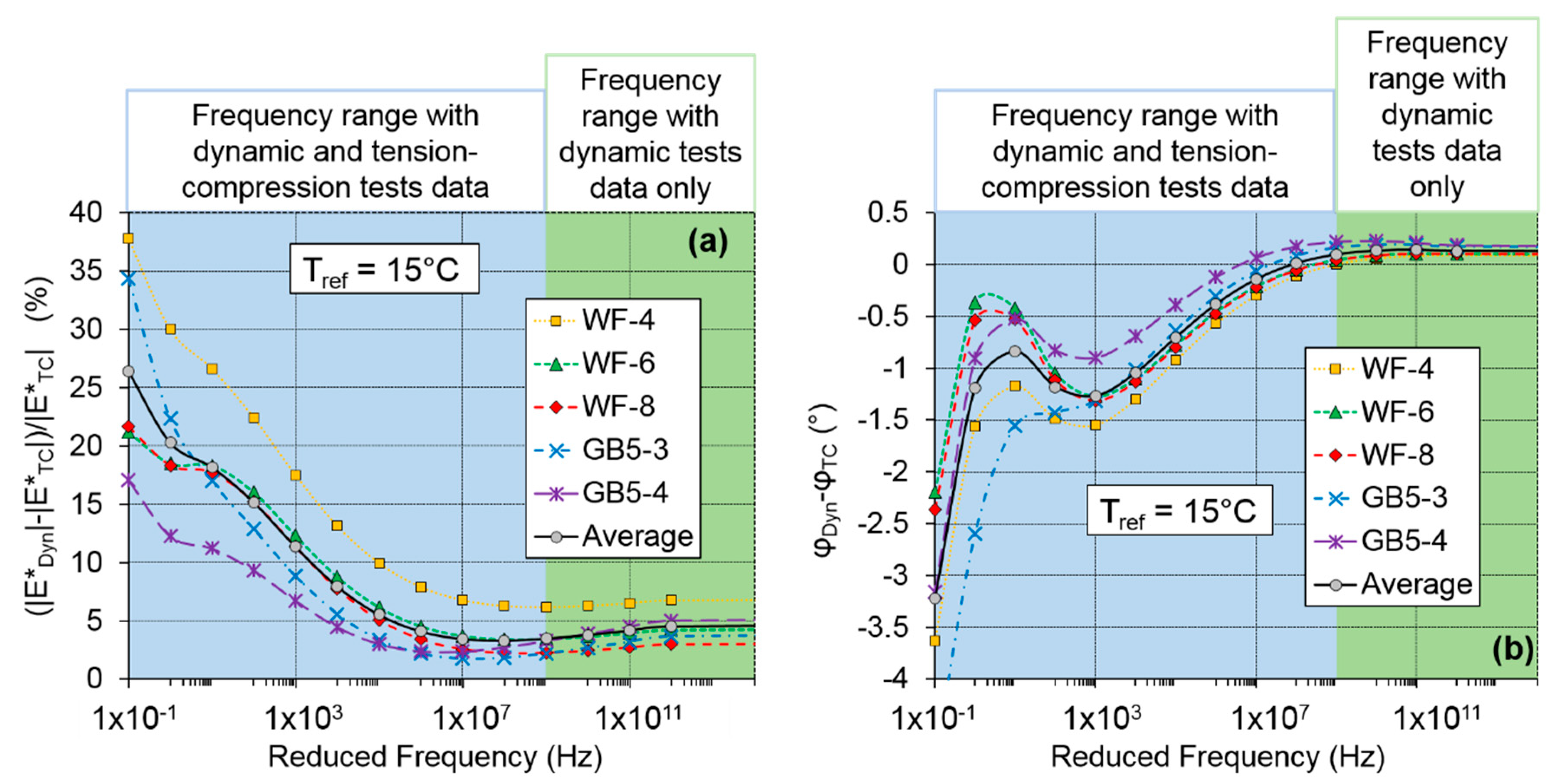
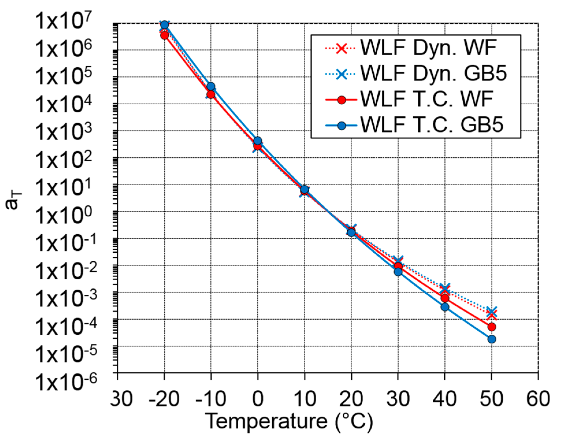
5.3. Comparison between Cyclic and Dynamic Tests Results

The reduced frequency range of the tension–compression and dynamic tests is different, as confirmed in Figure 10 and Figure 11. The tension–compression tests cover a reduced frequency range between approximately 10⁻⁷ Hz to 10⁹ Hz at a reference temperature of 15 °C. The dynamic tests cover a reduced frequency range between approximately 1 Hz and 10¹² Hz at the same reference temperature of 15 °C. Therefore, the best fit between the two tests is expected to be for frequencies higher than 1 Hz and lower than 10⁹ Hz for which experimental data from the two tests is available. As the two methods of back analysis of the dynamic tests give similar results, only the complex modulus obtained from the 2S2P1D model calibrated using the second method of analysis was chosen for the comparison with results of the 2S2P1D model calibrated from quasi-static tension–compression tests data. The relative difference between the norm (in %) and the phase (in °) of the complex modulus from the two calibration processes are plotted in Figure 14 where the results are plotted against the reduced frequency at 15 °C for all specimens. It is shown in Figure 14 that the complex modulus simulated from the two tests are in quite good agreement for the high reduced frequencies (>10⁷ Hz), which was expected when dealing with dynamic measurements. The norm of the dynamic complex modulus is around 3–5% higher than the norm of the complex modulus of the tension–compression tests for this frequency range and there is less than 0.2° of difference between the phase angles from both tests. For lower reduced frequencies (or higher temperatures), the relative difference increases for the norm and reach a value between 12% and 30% at 1 Hz depending on the specimen with an average value of 20.2%. The difference also increases for the phase angle but remains less than 2.5° for reduced frequencies higher than 1 Hz.

The differences observed in Figure 14 show that the dynamic complex modulus has a higher norm and a lower phase angle than the complex modulus obtained from the tension–compression tests. The differences between the two tests increase with temperature. These results are in agreement with results from previous studies using FRFs [18,19,20,21]. The differences between the two tests could be due to two phenomena. First, the level of strain applied is different in the two types of tests (about 50 μm/m for the tension–compression tests and about 0.1 μm/m for the dynamic tests). It is known that AM have a nonlinear behaviour showing a strain level dependence even at small strain amplitude [39,40,41]. The differences observed in this analysis are in the same direction than the observed nonlinearity: increasing of norm and decreasing of phase angle when decreasing strain amplitude. Then, nonlinearity may account for at least a part of the difference between the two tests. Another possibility is ageing of the materials. The tension–compression tests were performed several months before the dynamic tests and this could explain why the dynamic complex modulus is stiffer. However, the overall agreement between the two tests is satisfying.

The shift factors from the WLF equation obtained from the tension–compression tests and from the dynamic tests are plotted in Figure 15. It is seen that, for the low temperatures, the agreement between the shift factors from both tests is very good. For temperatures higher than 10 °C, the shift factors of the dynamic tests tend to be higher than the shift factors of the cyclic tests and the difference increases with temperature. The difference between the shift factors is more important for material labelled GB5. However, there is no apparent link between the difference observed in Figure 14 for the complex modulus and for the shift factors since the highest difference on the complex modulus evaluation correspond to a specimen of material labelled WF.

6. Conclusions

In this paper, conventional cyclic tension–compression tests and dynamic tests were performed to characterize the LVE behaviour of AM on a large range of frequencies and temperatures. Two different AM and five specimens were tested with both tests and results were analysed using the 2S2P1D model.

Two methods were studied to back-calculate the complex modulus of AM from dynamic measurements at each temperature. It is shown that the same shift factors are found with the two methods. Moreover, the two methods give very similar complex modulus values (less than 4% of difference for the norm of the modulus and 0.03° for the phase angle) and the differences observes may be due to the different assumptions on the Poisson’s ratio value. Therefore, the second method, which is a new and simpler approach, appears to be a good option to obtain the complex modulus of AM from FRFs.

The results of dynamic tests were also compared to the results of tension–compression tests. The shift factors from both tests are very close for the low temperatures and shift factors from dynamic tests are little higher for temperatures higher than 10 °C. The complex modulus obtained from dynamic tests have a higher norm and a lower phase angle than the ones determined with the conventional approach using cyclic tests. The differences observed between the two tests are very limited for the high frequencies or low temperatures (less than 5% for the norm and 0.2° for the phase angle) and are more important for the low frequencies or high temperatures (around 20% for the norm and 2° for the phase angle at 15 °C and 1 Hz). Since the strain level is approximately 500 times lower in the dynamic tests, the nonlinearity of AM with the level of strain amplitude may explain a part of the differences. Ageing of the materials between the tension–compression and the dynamic tests may also have an impact on the complex modulus evaluation.

The agreement between dynamic tests and the tension–compression tests is still satisfactory on the whole frequency range. The combination of the two tests methods is useful to improve the characterization of the LVE behaviour of AM on a wider frequency range because dynamic tests give access to very high frequencies. The presented research shows that dynamic tests, which have the great advantage of being cheap and rapid, can be back-analysed with a very simple model and can provide accurately the complex modulus of AM on a wide range of frequencies and temperatures.

References

1. Di Benedetto, H.; Corte, J.F. Matériaux Routiers Bitumineux 2: Constitution et Propriétés Thermomécaniques des Mélanges; Lavoisier: Paris, France, 2005; p. 288. (In French) [Google Scholar]
2. Halvorsen, W.G.; Brown, D.L. Impulse technique for structural response frequency testing. J. Sound Vib. 1977, 11, 8–21. [Google Scholar] [CrossRef]
3. ASTM: C215-08. Standard Test Method for Fundamental Transverse, Longitudinal and Torsional Frequencies of Concrete Specimens; ASCE: West Conshoshocken, PA, USA, 2008. [Google Scholar]
4. Migliori, A.; Sarrao, J. Resonant Ultrasound Spectroscopy-Applications to Physics, Materials Measurements and Nondestructive Evaluation; Wiley-Interscience Publication: New York, NY, USA, 1997. [Google Scholar]
5. Renault, A.; Jaouen, L.; Sgard, F. Characterization of elastic parameters of acoustical porous materials from beam bending vibrations. J. Sound Vib. 2010, 330, 1950–1963. [Google Scholar] [CrossRef]
6. Di Benedetto, H.; Sauzéat, C.; Sohm, J. Stiffness of bituminous mixtures using ultrasonic wave propagation. Road Mater. Pavement Des. 2009, 10, 789–814. [Google Scholar] [CrossRef]
7. Mounier, D.; Di Benedetto, H.; Sauzéat, C. Determination of bituminous mixtures linear properties using ultrasonic wave propagation. Constr. Build. Mater. 2012, 36, 638–647. [Google Scholar] [CrossRef]
8. Norambuena-Contreras, J.; Castro-Fresno, D.; Vega-Zamanillo, A.; Celay, M.; Lombillo-Vozmediano, I. Dynamic modulus of asphalt mixture by ultrasonic direct test. NDT E Int. 2010, 43, 629–634. [Google Scholar] [CrossRef]
9. Kweon, G.; Kim, Y.R. Determination of the complex modulus of asphalt concrete using the impact resonance test. J. Transp. Res. Board 2006, 1970, 151–160. [Google Scholar] [CrossRef]
10. Lacroix, A.; Kim, Y.R.; Far, M.S.S. Constructing the dynamic modulus mastercurve using impact resonance testing. J. Assoc. Asphalt Paving Technol. 2009, 78, 67–102. [Google Scholar]
11. Whitmoyer, S.L.; Kim, Y.R. Determining asphalt concrete properties via the impact resonant method. J. Test. Eval. 1994, 22, 139–148. [Google Scholar] [CrossRef]
12. Gudmarsson, A.; Ryden, N.; Birgisson, B. Application of resonant acoustic spectroscopy to asphalt concrete beams for determination of the dynamic modulus. Mater. Struct. 2012, 45, 1903–1913. [Google Scholar] [CrossRef]
13. Leisure, R.; Willis, F. Resonant ultrasound spectroscopy. J. Phys. Condens. Matter 1999, 9, 6001–6029. [Google Scholar] [CrossRef]
14. Ostrovsky, L.; Lebedev, A.; Matveyev, A.; Popatov, A.; Sutin, A.; Soustova, I.; Johnson, P. Application of three-dimensional resonant acoustic spectroscopy method to rock and building materials. J. Acoust. Soc. Am. 2001, 110, 1770–1777. [Google Scholar] [CrossRef] [PubMed]
15. Ryden, N. Resonant frequency testing of cylindrical asphalt samples. Eur. J. Environ. Civ. Eng. 2011, 15, 587–600. [Google Scholar] [CrossRef]
16. Ren, Z.; Atalla, N.; Ghinet, S. Optimization based identification of the dynamic properties of linearly viscoelastic materials using vibrating beam techniques. ASME J. Vib. Acoust. 2011, 133, 041012. [Google Scholar] [CrossRef]
17. Rupitsch, S.J.; Ilg, J.; Sutor, A.; Lerch, R.; Döllinger, M. Simulation based estimation of dynamic mechanical properties for viscoelastic materials used for vocal fold models. J. Sound Vib. 2011, 330, 4447–4459. [Google Scholar] [CrossRef]
18. Gudmarsson, A.; Ryden, N.; Birgisson, B. Characterizing the low strain complex modulus of asphalt concrete specimens through optimization of frequency response functions. J. Acoust. Soc. Am. 2012, 132, 2304–2312. [Google Scholar] [CrossRef] [PubMed]
19. Gudmarsson, A.; Ryden, N.; Di Benedetto, H.; Sauzéat, C.; Tapsoba, N.; Birgisson, B. Comparing Linear Viscoelastic Properties of Asphalt Concrete Measured by Laboratory Seismic and Tension-Compression Tests. J. Nondestruct. Eval. 2014, 33, 571–582. [Google Scholar] [CrossRef]
20. Gudmarsson, A.; Ryden, N.; Di Benedetto, H.; Sauzéat, C. Complex modulus and complex Poisson’s ratio from cyclic and dynamic modal testing of asphalt concrete. Constr. Build. Mater. 2015, 88, 20–31. [Google Scholar] [CrossRef]
21. Carret, J.-C.; Pedraza, A.; Di Benedetto, H.; Sauzéat, C. Comparison of the 3-dim linear viscoelastic behavior of asphalt mixes determined with tension-compression and dynamic tests. Constr. Build. Mater. 2018, 174, 529–536. [Google Scholar] [CrossRef]
22. Carret, J.-C.; Di Benedetto, H.; Sauzéat, C. Multi-modal dynamic linear viscoelastic back analysis for asphalt mixes. J. Nondestruct. Eval. 2018, 37, 35. [Google Scholar] [CrossRef]
23. Poirier, J.E.; Pouget, S.; Leroy, C.; Delaporte, B. Projets Mure et Improvmure: Bilan à mi-parcours. Revue Générale des Routes et de l’Aménagement 2016, 937, 38–41. (In French) [Google Scholar]
24. Gayte, P.; Di Benedetto, H.; Sauzéat, C.; Nguyen, Q. Influence of transient effects for analysis of complex modulus tests on bituminous mixtures. Road Mater. Pavement Des. 2015, 17, 271–289. [Google Scholar] [CrossRef]
25. Graziani, A.; Di Benedetto, H.; Perraton, D.; Sauzéat, C.; Hofko, B.; Poulikakos, L.; Pouget, S. Recommendation of RILEM TC 237-SIB on complex Poisson’s ratio characterization of bituminous mixtures. Mater. Struct. 2017, 50, 142. [Google Scholar] [CrossRef]
26. Perraton, D.; Di Benedetto, H.; Sauzéat, C.; Hofko, N.; Graziani, A.; Nguyen, Q. 3 Dim experimental investigation of linear viscoelastic properties of bituminous mixtures. Mater. Struct. 2016, 49, 4813–4829. [Google Scholar] [CrossRef]
27. Di Benedetto, H.; Olard, F.; Sauzéat, C.; Delaporte, B. Linear viscoelastic behavior of bituminous materials: From binders to mixtures. Road Mater. Pavement Des. 2004, 5, 163–202. [Google Scholar] [CrossRef]
28. Olard, F.; Di Benedetto, H. General 2S2P1D model and relation between the linear viscoelastic behaviors of bituminous binders and mixes. Road Mater. Pavement Des. 2003, 4, 185–224. [Google Scholar] [CrossRef]
29. Tiouajni, S.; Di Benedetto, H.; Sauzéat, C.; Pouget, S. Approximation of linear viscoelastic model in the 3 dimensional case with mechanical analogues of finite size—Application to bituminous materials. Road Mater. Pavement Des. 2011, 12, 897–930. [Google Scholar] [CrossRef]
30. Di Benedetto, H.; Delaporte, B.; Sauzéat, C. Three dimensional linear behavior of bituminous materials: Experiments and modeling. ASCE Int. J. Geomech. 2007, 7, 149–157. [Google Scholar] [CrossRef]
31. Nguyen, H.M.; Pouget, S.; Di Benedetto, H.; Sauzéat, C. Time-temperature superposition principle for bituminous mixtures. Eur. J. Environ. Civ. Eng. 2009, 13, 1095–1107. [Google Scholar] [CrossRef]
32. Nguyen, M.L.; Sauzéat, C.; Di Benedetto, H.; Tapsoba, N. Validation of the time–temperature superposition principle for crack propagation in bituminous mixtures. Mater. Struct. 2013, 46, 1075–1087. [Google Scholar] [CrossRef]
33. Nguyen, Q.T.; Di Benedetto, H.; Sauzéat, C.; Tapsoba, N. Time-temperature superposition principle validation for bituminous mixes in the linear and nonlinear domain. ASCE J. Mater. Civ. Eng. 2013, 25, 1181–1188. [Google Scholar] [CrossRef]
34. Ferry, J.D. Viscoelastic Properties of Polymers, 3rd ed.; John Wiley & Sons: New York, NY, USA, 1980. [Google Scholar]
35. Brüggemann, T.; Biermann, D.; Zabel, A. Development of an automatic modal pendulum for the measurement of frequency responses for the calculation of stability charts. Procedia CIRP 2015, 33, 587–592. [Google Scholar] [CrossRef]
36. Norman, P.E.; Jung, G.; Ratcliffe, C.; Crane, R.; Davis, C. Development of an Automated Impact Hammer for Modal Analysis of Structures; DSTO-TN-1062; DSTO Defence Science and Technology Organisation: Fishermans Bend, Australia, 2012. [Google Scholar]
37. Mangiafico, S.; Di Benedetto, H.; Sauzéat, C.; Olard, F.; Pouget, S.; Planque, L. New method to obtain viscoelastic properties of bitumen blends from pure and RAP binder constituents. Road Mater. Pavement Des. 2014, 15, 312–329. [Google Scholar] [CrossRef]
38. Pouget, S.; Sauzéat, C.; Di Benedetto, H.; Olard, F. Modeling of viscous bituminous wearing course materials on orthotropic steel deck. Mater. Struct. 2012, 45, 1115–1125. [Google Scholar] [CrossRef]
39. Airey, G.; Rahimzadeh, B. Combined bituminous binder and mixture linear rheological properties. Constr. Build. Mater. 2004, 18, 535–548. [Google Scholar] [CrossRef]
40. Nguyen, Q.T.; Di Benedetto, H.; Sauzéat, C. Linear and nonlinear viscoelastic behavior of bituminous mixtures. Mater. Struct. 2015, 48, 2339–2351. [Google Scholar] [CrossRef]
41. Mangiafico, S.; Babadopoulos, L.; Di Benedetto, H.; Sauzéat, C. Nonlinearity of bituminous mixtures. Mech. Time-Depend. Mater. 2018, 22, 29–49. [Google Scholar] [CrossRef]
Figure 1. Tension–compression test set-up (ENTPE laboratory, University of Lyon).
Applsci 08 02117 g001
Figure 2. Test set up for the dynamic impact tests (example for specimen WF-6, ENTPE laboratory, University of Lyon).
Applsci 08 02117 g002
Figure 3. Dynamic test experimental data for specimen GB5-3 at 14.7 °C (5 hits): (a) force in time domain; (b) acceleration in time domain; (c) force in frequency domain; and (d) acceleration in frequency domain.
Applsci 08 02117 g003
Figure 4. FRFs obtained for the 5 hits and averaged FRF (Equation (8)) of specimen GB5-3 at 14.7 °C.
Applsci 08 02117 g004
Figure 5. Coherence functions obtained for specimen GB5-3 at the five tested temperatures (a); and zoom on the lower frequencies (b).
Applsci 08 02117 g005
Figure 6. Finite element mesh and boundary conditions used for the FEM calculation of the FRFS.
Applsci 08 02117 g006
Figure 7. Method 1: Principle of the optimization procedure to identify the four 2S2P1D constants (E0, k, δ and τE) at each temperature. Xf is the final vector of the four 2S2P1D constants to identify.
Applsci 08 02117 g007
Figure 8. Influence of: E (a); ϕ (b); and ν (c) on the first peak of the FRFs corresponding to the first resonance (example of calculations for a cylinder with a 7.5 cm diameter and a 12.3 cm length).
Applsci 08 02117 g008
Figure 9. Method 2: Principle of the back-calculation of the complex modulus on the first resonance peak at each temperature (example for specimen GB5-3 at −0.2 °C).
Applsci 08 02117 g009
Figure 10. Summary and differences between the two proposed methods of back-analysis of the dynamic tests.
Applsci 08 02117 g010
Figure 11. Tension–compression test results and fitted 2S2P1D model for specimen WF-8: (a) Cole–Cole diagram; and (b) master curve for the norm of the complex modulus at 15 °C.
Applsci 08 02117 g011
Figure 12. Dynamic test results and fitted 2S2P1D model curve for the two analysis methods for specimen WF-8: (a) Cole–Cole diagram; and (b) master curve for the norm of the complex modulus at 15 °C.
Applsci 08 02117 g012
Figure 13. Difference between the complex modulus obtained from the two methods of analysis of the dynamic tests plotted at a reference temperature of 15 °C for all specimens: (a) relative difference for the norm of the complex modulus (in %); and (b) difference for the phase of the complex modulus (in °).
Applsci 08 02117 g013
Figure 14. Relative difference between the complex modulus simulated with the 2S2P1D model calibrated from back-calculation of the dynamic tests and the complex modulus simulated with the 2S2P1D model calibrated on the data of the tension–compression tests at 15 °C for all specimens: (a) relative difference for the norm of the complex modulus (in %); and (b) relative difference for the phase of the complex modulus (in °).
Applsci 08 02117 g014
Figure 15. Shift factors of the WLF equation (Equation (7)) obtained from the tension–compression tests (WLF T.C.) and from the dynamic tests (WLF Dyn.) for the two tested materials.
Applsci 08 02117 g015