Article

Designing a Diving Protocol for Thermocline Identification Using Dive Computers in Marine Citizen Science

1
Research Department, DAN Europe Foundation, 64026 Roseto degli Abruzzi, Italy
2
Department of Computer Engineering, MTF, Galatasaray University, Istanbul 34349, Turkey
3
Cousteau Divers, 75017 Paris, France
4
Department of Life and Environmental Sciences—DiSVA, Università Politecnica delle Marche, 60131 Ancona, Italy
*
Authors to whom correspondence should be addressed.
Submission received: 17 September 2018 / Revised: 19 October 2018 / Accepted: 29 October 2018 / Published: 20 November 2018

Abstract

:
Dive computers have an important potential for citizen science projects where recreational SCUBA divers can upload the depth temperature profile and the geolocation of the dive to a central database which may provide useful information about the subsurface temperature of the oceans. However, their accuracy may not be adequate and needs to be evaluated. The aim of this study is to assess the accuracy and precision of dive computers and provide guidelines in order to enable their contribution to citizen science projects. Twenty-two dive computers were evaluated during real ocean dives for consistency and scatter in the first phase. In the second phase, the dive computers were immersed in sufficient depth to initiate the dive record inside a precisely controlled sea aquarium while using a calibrated device as a reference. Results indicate that the dive computers do not have the accuracy required for monitoring temperature changes in the oceans, however, they can be used to detect thermoclines if the users follow a specific protocol with specific dive computers. This study enabled the authors to define this protocol based on the results of immersion in two different sea aquarium tanks set to two different temperatures in order to simulate the conditions of a thermocline.

1. Introduction

Temperature data from the oceans are very important to understand the ecosystems and assess the human impact on nature. There is large scale monitoring of sea surface temperature using both remote sensing and in-situ platforms [1,2,3,4], but there is a lack of depth resolved temperature profiles for inshore regions, besides the use of ‘animals of opportunity’ [5,6] and human volunteers [7,8] which help to monitor the depths/temperature profile data to address this issue. In fact, Citizen Science (CS) is becoming a powerful tool, bringing together scientists, society and decision makers. Recent reviews show that the last decades have seen a tremendous increase in CS projects and participation, thanks to technological advances amongst other elements. CS projects have also made contributions to science [9,10,11,12]. Recreational SCUBA divers are one of the important contributors to marine citizen science. Their key instrument is a dive computer (DC) that they need to use in order to monitor depth, time and in some models the amount of gas remaining in their tank. Dive computers include algorithms to predict the likelihood of decompression sickness and calculate the safe ascent rate for a diver. For that reason, the modern electronic DC can be considered as the most significant advancement in diving since the invention of the Aqualung by J.Y. Cousteau. Modern dive computers include an interface to allow the upload of the log of the dive to a mobile device or a desktop computer. Although there are standards on the accuracy and precision of dive computers (EN 13319) [13], one must be careful while using their output in scientific study. The use of this data will depend on the scientific question in mind. For example, there may be scenarios where an error of 1 °C is unacceptable, in which case improvements need to be made in the accuracy and consistency of dive computer temperature recordings [14].
Azzopardi and Sayer studied 47 dive computers and concluded that caution should be employed when using displayed and/or recorded depth and temperature data from dive computers in scientific or forensic studies [15]. Their conclusion on temperature is based on the deviation of up to 5.1 °C from nominal values. Caution is recommended for the use of dive computers as depth measurement tools in scientific study or underwater surveying.
Wright et al. reviewed the potential of SCUBA divers as oceanographic samplers when using their dive computers to augment aquatic temperature monitoring [14]. They have also attempted to use the temperature difference between surface and lowest temperatures recorded by the Operational Sea Surface Temperature and Sea Ice Analysis database [1] and the conductivity, temperature and density instruments respectively, to provide an idea of the degree of error of temperature recordings of dive computers. Their findings agreed with the results from Azzopardi and Sayer [15]. The overall outcome indicated that in a range of test temperatures between 10 and 17 °C, the median variance was 5.1 °C (with a range of −4.0 to 1.1 °C). Furthermore, they concluded that identification of the depth of the thermocline is likely to be possible in the future with a more structured collection of data, but will depend on the strength of the thermocline and the quality of the dive computer.
The aim of this study is to simulate the thermocline with a pair of sea aquarium basins and determine the protocol to be used to detect the thermoclines using the dive computer logs.

2. Methods

2.1. Open Water Dive

Prior to controlled experiments in a sea aquarium, a SCUBA dive is planned to verify if the dive computers are functioning properly. The Bosporus Channel dive site was selected, where the thermocline due to the counter flow of Mediterranean and Black Sea water is commonly observed at varying depths and locations. Gregg et al. found the exchange flow between the Sea of Marmara and the Black Sea to be quasi-steady. The dive site was selected as a potential point to observe the temperature gradients [16]. A team of 3 divers made a dive to 49 m for a total dive time of 16 min while carrying 21 dive computers attached to acrylic rods (Figure 1).
At the end of the dive, depth, time and temperature profile data was uploaded to a desktop computer and was converted to CSV format using Subsurface, an open-source software released under the GPLv2 license [17]. The data was also uploaded to the Diving Safety Laboratory database (DSL-DB) using the Diving Safety Guardian portal for future processing, both for oceanographic and diving medicine research. Divers Alert Network Europe (DAN) created a database (DB) with a large amount of dive related data, which has been collected since 1994 within the scope of the Dive Safety Laboratory (DSL) project. These dive profiles were collected from different models of diving computers and converted into the original DAN DB format known as DAN DL7, which became the industry standard for dive profile data exchange, and many manufacturers are now embedding a DL7 compliant data download option in their dive computers. DSL hosts 70,008 dive profiles as of May 2017, uploaded by 5659 divers [18]. A special section in DSL DB was created for the analysis of undersea temperature data for a future project to identify thermoclines, especially in the Mediterranean Sea. The dive described above is the first dive uploaded for that purpose.

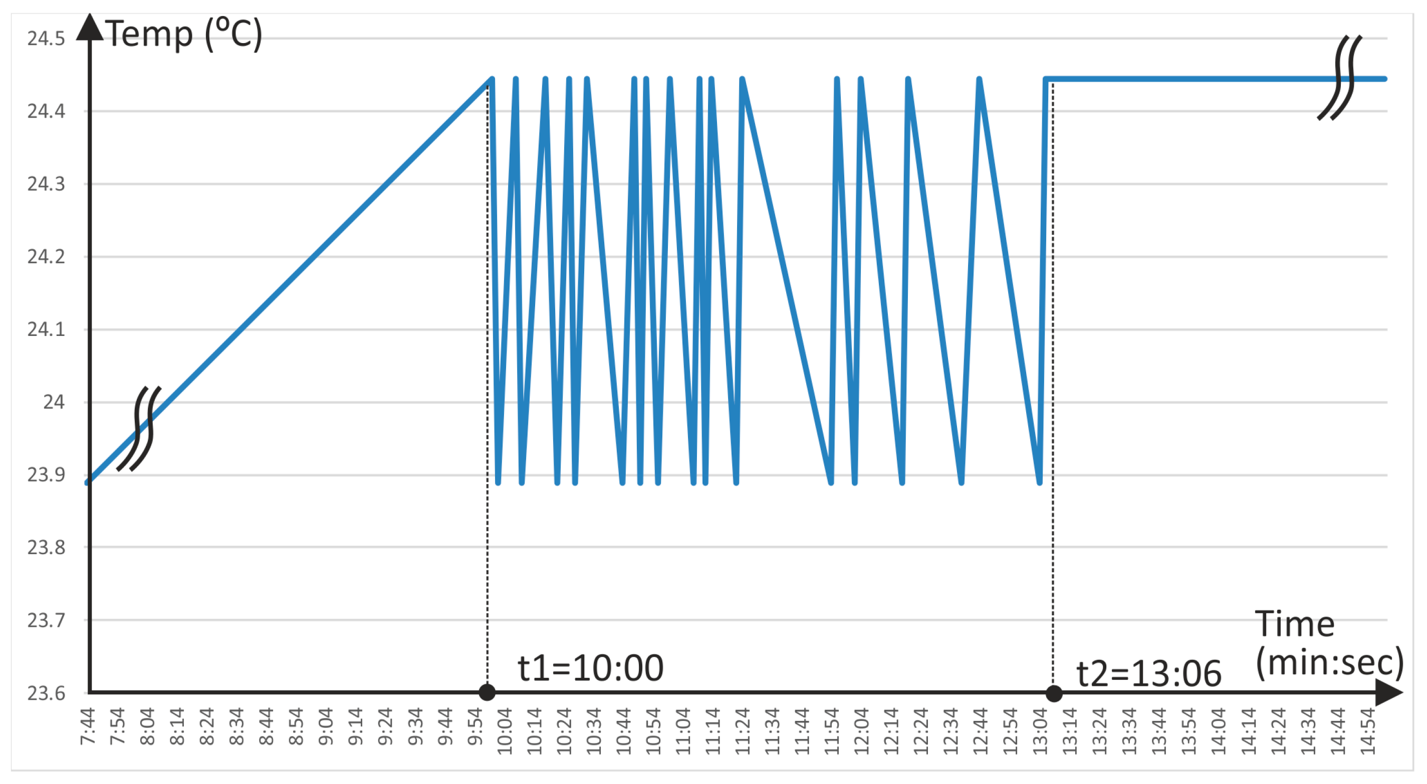
2.2. Sea Aquarium Experiments

Sea aquariums were selected in order to obtain a controlled environment with a high volume of water where the temperature is stable and will not be biased by the temperature of the dive computers. At the experiment site, the Panama (AQ1) and Pacific (AQ2) tanks of Istanbul Aquarium (Istanbul, Turkey) are equipped with high precision thermostats coupled to heaters and are stabilized at 17 °C and 25.5 °C, respectively. The tanks were chosen to have sufficient depth, as dive computers need a minimum depth to trigger the depth/temperature profile logging. The minimum depth is different for each manufacturer but ranges from 80 cm to 120 cm. In this experiment, the immersion was at least 1.8 m in order to ensure the activation of the dive computers, and the proper startup of the dive computers was checked by a diver (Figure 2). The distance between the aquariums was about 50 m and at the end of each immersion the dive computers were carried inside a bucket containing water at the stabilized temperature of the aquarium in order to prevent cooling during transport.
The following describes two experiments to simulate the passage of a diver through a thermocline layer while descending and ascending. The first phase is designed for stabilization of initial conditions and is not used for modeling the DC response. The stay in each aquarium was extended to one hour in order to observe, and if possible, model the latency of the dive computers by measuring the temperature (Figure 3a,b). The reference temperature was measured by a laboratory grade instrument (556 Handheld Multi parameter, YSI Incorporated, Yellow Springs, OH, USA) calibrated by the accredited laboratory of the Turkish Standards Institute. Dive profiles were downloaded following the same procedure as the open water dives in the Bosporus Channel.
The dive computers were kept for one hour in AQ1 and were immersed in AQ2 for another hour and immersed again in AQ1 for another 60 min. Periods 1 and 2 were used for modeling the dive computers.

3. Results

During the open water dives, three dive computers failed: Two had download problems while one shut down during the dive. Hence, Experiment 1 in the aquarium involved 18 computers while Experiment 2 involved 19, because the one that shut down during the dive had recovered after a firmware update. The dive computers with download problems were eliminated from the experiments.
The downloaded depth and temperature data from the open water dives in Bosporus is given in Figure 4. A similar degree of scatter is observed by Wright et al. [14] and Azzopardi and Sayer [15].
The temperature-time profiles of the experiment 1 and 2 are given in Figure 5 and Figure 6 respectively. Most of the DCs display an exponential change which can be modeled using the classical equation that is the solution of a first order system:
T (t) = C + A (1 − e−kt)
where T is temperature in Celsius, t is time in minutes, 1/k is the time constant (the amount of time it takes for temperature values to change approximately 63.2% from their starting values to their final values in a transient situation) of the system. C is the initial temperature and A is the step change in temperature. Based on this assumption, the curve fitting by least squares method was applied to each DC to find the time constant (Table 1). 1/k and R2 values were calculated for periods 1, 2, 3 and 4 and the experiments and the results are listed in Table 1 for 14 DCs. In Figure 7, a sample curve fitting graph, where the blue line was generated according to measured temperature values and the red line was generated according to temperatures values calculated using the function (1) is displayed.
Most of the DCs fit equation E1 with a high confidence (R2 > 0.9 for 41 curves out of 56) while time constants range from 7 to 280 s. Four curves resulted in a very poor fit and are indicated by italic numbers in Table 1. As expected, the time constants for periods 1–4 and 2–3 yielded similar results. According to these results, if a diver stays more than 3 min at a depth where the temperature exhibits a stepwise change (thermocline), a noticeable change in temperature of around 50% will be observed from the log of a DC. The resulting protocol for divers is described below:
Step 1. Mark the geolocation of the dive site.
Step 2. Make sure that the DC time and date are set correctly.
Step 3. Mark the DC model and serial number.
Step 4. During the pre-dive briefing, if dive team members are not familiar with the CS project, inform them that you will stop for at least 3 min to mark the thermocline.
Step 5. Before the dive, avoid exposing your DC to extreme temperature differentials; if possible, let it be immersed in water at a depth shallower than the one that triggers depth profile logging and decompression computing (30 cm is an adequate depth to immerse for most of the available DCs in the market).
Step 6. During the dive, when you will stop for at least 3 min, make sure that this stop does not impose any danger to you and other team members. Such dangers might include but not limited to disadvantageous decompression obligations, drifting with the current or boat accidents.
Step 7. Do not limit your contribution with a single dive at the same location. If possible, provide multiple dive data samples for the same location.

4. Discussion

The Mediterranean Sea is considered a miniature ocean, able to mimic on a shorter time scale the dynamics of the world’s oceans. This model can be used as a giant mesocosm of the open oceans [19], with various impacts interacting synergistically [20].
Climate change, affecting the usual frequency and intensity of winds, rainfalls and temperature, is rapidly modifying the typical circulation pattern of the Mediterranean Sea. The thermal anomalies documented with an increasing frequency in the last 20 years are showing impressive effects on the distribution of marine organisms. The biodiversity of the Mediterranean Sea is considered incredibly high compared to other areas, owing to the unique and complex geological history of the basin. Owing to the Messinian crisis and the glacial ages, we found organisms with both a cold (northwestern basin) and warm (southeastern basin) affinity.
Climate change is creating many problems for species with a cold affinity who cannot adapt to the new thermal regime, and it is enhancing the distribution of warmwater species.
Throughout the year the Mediterranean Sea is characterized by a typical thermic cycle, reflecting the parallel distribution of nutrients and chlorophyll. The cycle is characterized by the establishment, during the summer season, of a thermocline that is a variable extended zone defined by a steep temperature gradient. For the marine environment, the thermocline depth is an ecological boundary, because it represents the level of the physiological thermic limit for many species. Nutrients, oxygen, and other limiting factors tend to accumulate near it.
Since the global thermal shift, which occurred as a consequence of the El Nino in 1998, the thermocline has been increasing its depth range and many species with a cold-affinity began to disappear from the upper layers in the North–Western basin. Mainly benthic filter feeders are affected by massive mortalities, rapidly changing the seascapes of many coastal areas [21,22,23].
Even if seawater temperature is only one of the parameters responsible for mortality outbreaks, knowing the precise position of the thermocline during the summer and autumn seasons could allow a better understanding and potentially be used to predict massive mortality events or other important biological processes.
The opportunities for researchers to collect this information on a wide spatial scale are very scarce. The contributions of recreational divers equipped with adequate computers could allow for the understanding of irregular patterns of mortality events that, with the poor spatial resolution currently available for seawater temperature close to the seafloor, remain without a clear explanation.
The suggested protocol of staying 3 min at the depth of the step change in temperature can detect all the simulated thermoclines of Experiment 1 and 2 but cannot detect the magnitude of the temperature shift. This protocol can be used to locate the depth and the geolocation if used together with dive logging software, such as eDiverlog (Pelagic Pressure Systems, San Leandro, CA, USA).
Further expectation on quantitative information of temperature may lead to erroneous data, since a dive computer’s primary aim is not to measure the temperature accurately. For instance, during Experiment 1, an oscillation of temperature was recorded by a dive computer, probably due to the insufficient digitization. The temperature of 24.15 °C is either quantified as 24.4 or 23.9, depending upon microclimate changes and due to poor discretization (Figure 8).
Divers generally are keen citizen scientists that are happy to collect information to help better understand the oceans [24,25]. This is confirmed by the unprecedented success of DSL in contribution to diving medicine [26]. The DSL DB now has a section for detecting thermoclines and is ready to accept data uploads from volunteers; however, a filter needs to be added to the web interface in order to check if the divers followed the correct protocol. That will open a new “the citizen science” channel for divers who want to contribute to oceanography.

5. Conclusions

Caution should be employed when using displayed and/or recorded depth and temperature data from dive computers in scientific studies. Based on the results, in order to tag the thermoclines, we suggest that divers stop for a minimum period of 3 min during descent if the diving conditions do not impose any stress including decompression. Our protocol is based on controlled experiments and provides a robust method of identifying the tempo-spatial distribution of Mediterranean thermoclines. This assessment is critical for environmental impact assessments and vital for initiating timely measures. The existence of DSL DB, with 5659 divers already enrolled, offers a promising infrastructure to launch this marine citizen science action for thermocline identification, enhanced by the Cousteau Divers network.

Author Contributions

Conceptualization: S.M.E., P.Y.C. and C.C.; Methodology: S.M.E., C.C. and T.Ö.; Investigation: S.M.E., P.Y.C., M.P. and T.Ö.; Data Curation: M.P. and C.C.; Formal Analysis: T.Ö.; Writing—Original Draft: S.M.E.; Writing—Review and Editing: S.M.E. and T.Ö.; Project Administration: S.M.E. and A.M., Funding Acquisition: S.M.E. and A.M.

Funding

This study was funded by the Green Bubbles RISE project, H2020-MSCA-RISE-2014. The project has received funding from the European Union Horizon 2020 research and innovation programme under the Marie Sklodowska-Curie grant agreement No. 643712. This document reflects only the authors view. The Research Executive Agency is not responsible for any use that may be made of the information it contains.

Acknowledgments

Authors would like to express their gratitude to Ali Ethem Keskin who shot the underwater pictures. Authors would like to thank to the management of Istanbul Aquarium for their continuous help during the experiments.

Conflicts of Interest

The authors declare no conflict of interest.

References

  1. Stark, J.D.; Donlon, C.J.; Martin, M.J.; McCulloch, M.E. OSTIA: An operational, high resolution, real time, global sea surface temperature analysis system. In Proceedings of the OCEANS 2007—Europe, Aberdeen, UK, 18–21 June 2007; pp. 1–4. [Google Scholar]
  2. Roemmich, D.; Johnson, G.C.; Riser, S.; Davis, R.; Gilson, J.; Owens, W.B.; Garzoli, S.L.; Schmid, C.; Ignaszewski, M. The Argo Program: Observing the global oceans with profiling floats. Oceanography 2009, 22, 34–43. [Google Scholar] [CrossRef]
  3. Rudnick, D.L.; Cole, S.T. On sampling the ocean using underwater gliders. J. Geophys. Res. 2011, 116. [Google Scholar] [CrossRef] [Green Version]
  4. Kennedy, J.J.; Rayner, N.A.; Smith, R.O.; Parker, D.E.; Saunby, M. Reassessing biases and other uncertainties in sea surface temperature observations measured in situ since 1850: 1. Measurement and sampling uncertainties. J. Geophys. Res. 2011, 116. [Google Scholar] [CrossRef] [Green Version]
  5. Charrassin, J.-B.; Park, Y.-H.; Le Maho, Y.; Bost, C.-A. Fine resolution 3D temperature fields off Kerguelen from instrumented penguins. Deep Sea Res. Part I Oceanogr. Res. Pap. 2004, 51, 2091–2103. [Google Scholar] [CrossRef]
  6. Simmons, S.E.; Tremblay, Y.; Costa, D.P. Pinnipeds as ocean-temperature samplers: Calibrations, validations, and data quality. Limnol. Oceanogr. Methods 2009, 7, 648–656. [Google Scholar] [CrossRef]
  7. Brewin, R.J.W.; de Mora, L.; Jackson, T.; Brewin, T.G.; Shutler, J. On the potential of surfers to monitor environmental indicators in the coastal zone. PLoS ONE 2015, 10, e0127706. [Google Scholar] [CrossRef] [PubMed] [Green Version]
  8. Joyce, A.E. The coastal temperature network and ferry route programme: Long-term temperature and salinity observations. Sci. Ser. Data Rep. Cefas Lowestoft 2006, 43, 129. [Google Scholar]
  9. Bonney, R.; Cooper, C.B.; Dickinson, J.; Kelling, S.; Phillips, T.; Rosenberg, K.V.; Shirk, J. Citizen science: A developing tool for expanding science knowledge and scientific literacy. Bioscience 2009, 59, 977–984. [Google Scholar] [CrossRef]
  10. Dickinson, J.L.; Shirk, J.; Bonter, D.; Bonney, R.; Crain, R.L.; Marin, J.; Phillips, T.; Purcell, K. The current state of citizen science as a tool for ecological research and public engagement. Front. Ecol. Environ. 2012, 10, 291–297. [Google Scholar] [CrossRef] [Green Version]
  11. Thiel, M.; Penna-Díaz, M.A.; Luna-Jorquera, G.; Salas, S.; Sellanes, J.; Stotz, W. Citizen scientists and marine research: Volunteer participants, their contributions, and projecIon for the future. Oceanogr. Mar. Biol. Annu. Rev. 2014, 52, 257–314. [Google Scholar]
  12. Collins, K.J.; Baldock, B. Use of diving computers in brittlestar surveys. Underw. Technol. 2007, 27, 115–118. [Google Scholar] [CrossRef]
  13. European Committee for Standardization. EN 13319, Diving Accessories—Depth Gauges and Combined Depth and Time Measuring Devices—Functional and Safety Requirements, Test Methods; European Standard Approved by CEN on 20 January 2000; BSI: London, UK, 2000. [Google Scholar]
  14. Wright, S.; Hull, T.; Sivyer, D.B.; Pearce, D.; Pinnegar, J.K.; Martin, D.J.; Sayer, M.D.J.; Mogg, A.O.M.; Azzopardi, E.; Gontarek, S.; et al. SCUBA divers as oceanographic samplers: The potential of dive computers to augment aquatic temperature monitoring. Sci. Rep. 2016, 6, 30164. [Google Scholar] [CrossRef] [PubMed] [Green Version]
  15. Azzopardi, E.; Sayer, M.D.J. A review of the technical specifications of 47 models of diving decompression computer. Underw. Technol. 2010, 29, 63–72. [Google Scholar] [CrossRef]
  16. Gregg, M.C.; Özsoy, E.; Latif, M.A. Quasi-steady exchange flow in the Bosphorus. Geophys. Res. Lett. 1999, 26, 83–86. [Google Scholar] [CrossRef]
  17. Subsurface. Available online: https://subsurface-divelog.org/ (accessed on 10 June 2018).
  18. Divers Safety Guardian. Available online: https://diversafetyguardian.org/ (accessed on 10 June 2018).
  19. Bethoux, J.P.; Gentili, B.; Morin, P.; Nicolas, E.; Pierre, C.; Ruiz-Pino, D. The Mediterranean Sea: A miniature ocean for climatic and environmental studies and a key for the climatic functioning of the North Atlantic. Progr. Oceanogr. 1999, 44, 131–146. [Google Scholar] [CrossRef]
  20. Micheli, F.; Halpern, B.S.; Walbridge, S.; Ciriaco, S.; Ferretti, F.; Fraschetti, S.; Lewison, R.; Nykjaer, L.; Rosenberg, A.A. Cumulative human impacts on Mediterranean and Black Sea marine ecosystems: Assessing current pressures and opportunities. PLoS ONE 2013, 8, e79889. [Google Scholar] [CrossRef] [PubMed] [Green Version]
  21. Cerrano, C.; Bavestrello, G.; Bianchi, C.N.; Cattaneo-Vietti, R.; Bava, S.; Morganti, C.; Morri, C.; Picco, P.; Sara, G.; Schiaparelli, S.; et al. A catastrophic mass-mortality episode of gorgonians and other organisms in the Ligurian Sea (North-western Mediterranean), summer 1999. Ecol. Lett. 2000, 3, 284–293. [Google Scholar] [CrossRef]
  22. Garrabou, J.; Coma, R.; Bensoussan, N.; Bally, M.; Chevaldonné, P.; Cigliano, M.; Diaz, D.; Harmelin, J.G.; Gambi, M.C.; Kersting, D.K.; et al. Mass mortality in Northwestern Mediterranean rocky benthic communities: Effects of the 2003 heat wave. Glob. Chang. Biol. 2009, 15, 1090–1103. [Google Scholar] [CrossRef]
  23. Rivetti, I.; Boero, F.; Fraschetti, S.; Zambianchi, E.; Lionello, P. Anomalies of the upper water column in the Mediterranean Sea. Glob. Planet Chang. 2017, 151, 68–79. [Google Scholar] [CrossRef]
  24. Nguyen, H.Y.; Pedersen, O.; Ikejima, K.; Sunada, K.; Oishi, S. Using Reefcheck monitoring database to develop the coral reef index of biological integrity. J. Fish. Aquat. Sci. 2009, 4, 90–102. [Google Scholar] [CrossRef]
  25. Pikesley, S.K.; Godley, B.J.; Latham, H.; Richardson, P.B.; Robson, L.M.; Solandt, J.; Trundle, C.; Wood, C.; Witt, M.J. Pink sea fans (Eunicella verrucosa) as indicators of the spatial efficacy of Marine Protected Areas in southwest UK coastal waters. Mar. Policy 2016, 64, 38–45. [Google Scholar] [CrossRef]
  26. Cialoni, D.; Pieri, M.; Balestra, C.; Marroni, A. Dive Risk Factors, Gas Bubble Formation, and Decompression Illness in Recreational SCUBA Diving: Analysis of DAN Europe DSL Data Base. Front. Psychol. 2017, 8, 1587. [Google Scholar] [CrossRef] [PubMed]
Figure 1. Open water tests with real dives (21 March 2018).
Applsci 08 02315 g001
Figure 2. Diver checking the proper booting of the dive computers.
Applsci 08 02315 g002
Figure 3. (a) Temperature profiles for Experiment 1; (b) temperature profiles for Experiment 2. The order of experiment 1 is inverted.
Applsci 08 02315 g003
Figure 4. Temperature and depth profiles for the dives in Bosporus. Solid lines are for depth and dotted lines are for temperature.
Applsci 08 02315 g004
Figure 5. The results of Experiment 1.
Applsci 08 02315 g005
Figure 6. The results of Experiment 2.
Applsci 08 02315 g006
Figure 7. Sample curve fit for the dive computer Mares Smart. The resulting time constant is 66.06 s with an R2 of 0.9877.
Applsci 08 02315 g007
Figure 8. Temperature oscillation as logged by a dive computer (Hollis TX1).
Applsci 08 02315 g008
Table 1. R2 and time constants for dive computers.
ComputerDive1/kR2
Hollis TX11208.76650.9947
2172.76610.7079
3165.09550.9414
4241.68720.9887
Mares Icon1136.42870.9986
2150.55660.9838
3200.00000.6915
4143.61420.9993
Mares Matrix182.58820.9928
234.08840.9113
370.92350.9514
451.66830.9688
Mares Smart176.51680.9810
224.07200.8914
375.54510.9832
465.06000.9877
Oceanic OC11152.56920.9916
25000.00000.0566
3153.09330.9118
4149.16150.9953
Oceanic Veo 2 No.11281.15420.9909
2170.81800.8137
3205.80480.9444
4265.78760.9874
Oceanic Veo 2 No.21279.56090.9876
295.23360.6806
3213.85640.9366
4261.96800.9879
Oceanic VT41236.36200.9915
2127.92180.8740
3265.28890.9582
4254.46230.9881
Sensus Ultra No.11194.95320.9998
2198.26940.9979
3213.81820.9998
4199.96270.9999
Sensus Ultra No.21192.06570.9998
2210.83710.9978
3202.13180.9998
4203.63781.0000
Suunto D4171.87810.9710
293.61150.8035
331.02850.8399
491.58160.9661
Suunto D61203.34330.8472
27.30990.9009
39.88250.7992
Suunto139.40320.9654
225.68030.3220
322.75050.0492
450.16220.9692
Uwatec Galileo Sol199.32890.9597
22.63560.0963
394.10560.8101
4102.14180.9663

