Investigation on Ship Hydroelastic Vibrational Responses in Waves

Abstract

The hydroelastic vibrational responses of a large ship sailing in regular and irregular head waves are investigated numerically and experimentally. A 3D time-domain nonlinear hydroelastic mathematical model is established in which the hydrostatic restoring forces and incident wave forces are calculated on the instantaneous wetted hull surface to consider nonlinear effects of the rigid motion and elastic deformation of the hull in harsh waves. Radiation and diffraction wave forces are computed on the mean wetted surface based on the 3D frequency-domain potential flow theory. The slamming loads are calculated by momentum theory and integrated into the hydrodynamic forces. The 1D Timoshenko beam theory is adopted to model the vibrational structural response and is fully coupled with the presented hydrodynamic theory in time-domain to generate the hydroelastic equation of motion. Moreover, self-propelled segmented model tests were conducted in a laboratory wave tank to experimentally investigate the hydroelastic responses of a target ship in regular and irregular head seas. The numerical and experimental results are systemically compared and analyzed, and the established hydroelastic analysis model turns out to be reliable and effective in the prediction of ship hydroelastic responses in waves.

1. Introduction

Structural evaluation of marine vessels during their design stage relies on accurate prediction of hydrodynamic loading and subsequent wave-structure interactions. For the cases where the elastic deformation of the structure plays a negligible role in determining the hydrodynamic forces, the structural analysis can be performed separately from the hydrodynamic analysis. However, large vessels with pronounced bow flare are susceptible to frequent and severe wave impact, subjecting them to subsequent significant transient hull vibrations, called whipping, which inevitably interferes with the surrounding fluid field and violates the basic assumption of the conventional decoupled method mentioned above. Hydroelasticity theory sufficiently considers the effects of structural vibrational responses on the hydrodynamic forces, and therefore, provides a framework in which structural and hydrodynamic analyses are fully coupled.

Research on robust and efficient numerical methods for evaluation of ship wave loads and structural responses is still in progress. Bishop and Price [1] first introduced the methodology of hydroelasticity into ship engineering, paving the way for the following fruitful development. Early research efforts mainly focused on 2D theories in which 2D strip theories, linear or nonlinear, are adopted to analyze the hydrodynamics, while the elastic responses of the ship are represented by the modal superposition method [2,3,4]. With the advent and popularization of high-performance computers, 3D hydroelastic analysis gradually captured the attention of the marine community, especially for the cases where the assumptions of the strip method are not appropriately satisfied [5,6]. The fluid flow is modeled by the 3D potential flow theory, and the ship structure is considered using a 1D or 3D finite element (FE) model [7,8,9]. Recently, Computational Fluid Dynamics (CFD) simulation of fluid flow has been incorporated into the methodology of hydroelasticity [10,11], but the immense amount of time required at present hinders the development of this process, and makes it impractical for use in practical engineering applications.

Together with the development of a theoretical approach is the experimental investigation. Small scale ship model tests in towing tanks have been widely conducted to study hydroelastic responses, such as vertical motions and bending moments, with the experimental conditions ranging from moderate seas to high seas [12,13,14]. Besides those small scale model tests, large scale model tests and even the full-scale ship tests have been conducted to further enhance the understanding of fluid-structure interaction mechanisms [15,16,17,18]. A benchmark study on the performance of seventeen hydroelastic analysis codes applied to a target containership was carried out [19]. The hydroelastic model experiment of the target containership was conducted to further test each seakeeping code. Comprehensive comparisons showed that the participating codes gave scattered results for severe sea conditions, indicating the need for further theoretical research and subsequent verification by experiments. Clauss and Klein [20] experimentally investigated the characteristics of vertical bending moments (M_BV) for different hulls in extreme seas. The analysis showed that large bow flares significantly affect the M_BVs.

The understanding and simulation of nonlinearities associated with hydroelastic vibrational responses of large vessels in high seas are the central task for the ship engineering community. The fierce fluid structure interaction is characterized by strongly nonlinear slamming, wave breaking, large amplitude ship motion, etc., posing great technical difficulties on the theoretical prediction of ship responses. More often than not, severe seas have highly-irregular wave conditions which make the characteristics of ship hydroelasticity very different from those in regular waves. Although there has been significant progress in the field of fluid structure interaction, the study of nonlinear hydroelastic responses of large ships in severe irregular sea conditions using 3D methodology is rather scarce in the present literature. Accordingly, the aim of the present paper is to systematically study the hydroelastic vibrational characteristics of a target large ship in both regular and irregular waves. A fully coupled 3D nonlinear hydroelastic method in the time domain is constructed to study whipping responses of a large ship with a pronounced bow flare in regular and irregular wave conditions. The structure of the vessel is idealized as a 1D Timoshenko beam, and the fluid flow is simulated by the 3D potential flow theory. Slamming loads are calculated based on the momentum method. An in-house hydroelastic analysis code is accordingly developed to predict ship responses in regular and irregular waves. To validate the numerical results, experimental tests of a target large ship in regular and irregular head waves were carried out in a towing tank. Quantitative time domain comparisons of numerical and experimental ship responses in regular head seas are discussed, with qualitative time domain comparisons of ship responses, statistical parameters, and probability of exceedance of response extrema being analyzed for ship short-term responses in irregular seas.

2. Ship Hydroelasticity Theory in Regular and Irregular Waves

2.1. Basic Assumption and Description

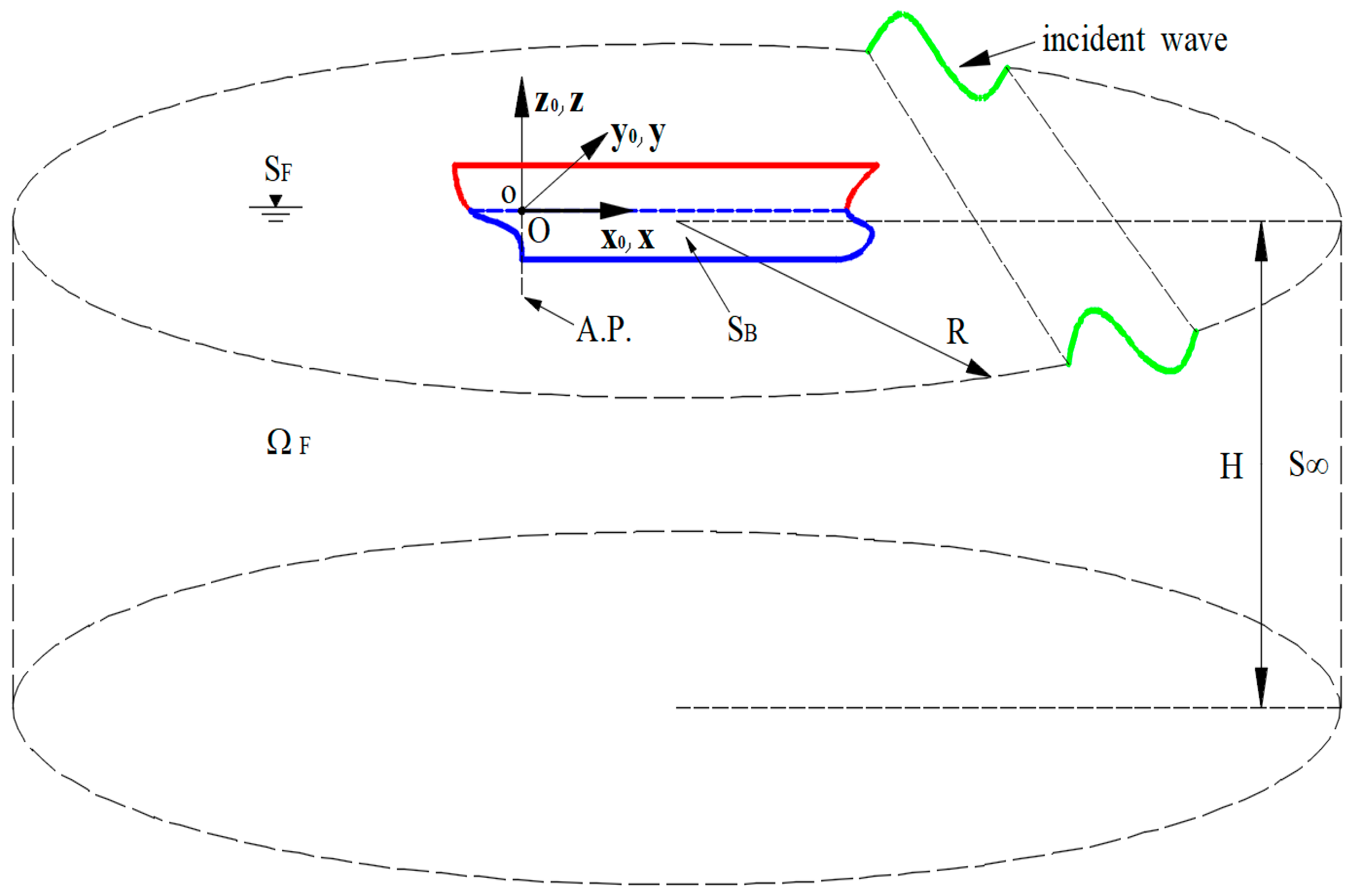
The general description of ship hydroelastic responses in regular or irregular waves is demonstrated in Figure 1. In the figure, the fluid field Ω_F is assumed to be infinite in the horizontal direction, with parameters R, H, S_∞, and S_F respectively being denoted as the infinite radius of Ω_F, the finite or infinite depth of Ω_F, the infinite boundary of Ω_F in the horizontal direction, and the free surface of Ω_F. S_B denotes the wet hull surface.

The earth fixed Cartesian frame Ox₀y₀z₀, the translational Cartesian frame oxyz, and the ship hull fixed Cartesian frame Gx_by_bz_b are adopted to study the fluid structure interaction problem. Initially, reference frames Ox₀y₀z₀ and oxyz are spatially identical. Coordinate planes Ox₀y₀ and oxy are at the calm waterplane with their origins being positioned at the After Perpendicular (A.P.). The translational Cartesian frame oxyz translates at the constant ship velocity U and keeps parallel to Ox₀y₀z₀. The hull fixed reference frame Gx_by_bz_b moves identically with the ship, and G is the Center of Gravity (CG) of the ship. The Galilean transformation relation between these three reference frames at any time t is shown below:

$$\left\{\begin{array}{c}x\\ y\\ z\end{array}\right\}=\left[\begin{array}{ccc}\cos \beta & \sin \beta & 0\\ -\sin \beta & \cos \beta & 0\\ 0& 0& 1\end{array}\right]\left\{\begin{array}{c}{x}_0\\ y_0\\ z_0\end{array}\right\}+\left\{\begin{array}{c}-Ut\\ 0\\ 0\end{array}\right\}\approx \left\{\begin{array}{c}{x}_b\\ y_b\\ z_b+z_G\end{array}\right\}$$

(1)

where β denotes the azimuth of the ship.

2.2. Hydroelastic Equation of Motion

Based on the modal superposition formulation [2], the hydroelastic equation of motion of a large vessel advancing in regular or irregular waves can be expressed as follows:

$$[m][\ddot{p}]+[c][\dot{p}]+[k][p]=[F_I]+[F_D]+[F_R]+[F_H]+[F_{SL}]$$

(2)

where [m], [c] and [k] are called generalized mass, damping, stiffness matrices, respectively. [p] denotes the principal coordinate matrix. All the five terms of the right-hand side of Equation (2) are called generalized force matrices, where [F_I], [F_D], [F_R], [F_H] and [F_SL] are the Froude-Krylov force matrix, diffraction force matrix, radiation force matrix, hydrostatic restoring force matrix, and slamming force matrix, respectively.

Even though the structural part of Equation (2) is based on the linear theory of solid mechanics, we can still obtain the nonlinear structural responses by practically taking into account the nonlinear effects of some of those five generalized force matrices. Those nonlinear effects should appropriately reveal the real physics of the fluid structure interaction whilst balancing this requirement against the consideration of time efficiency. Therefore, [F_I], [F_H] and [F_SL] are calculated on the instantaneous wet surface of the ship to include nonlinearities associated with hull geometry. In contrast, [F_D] and [F_R] are remained linear and computed based on the mean wet elastic ship surface in calm water. The following paragraphs will elaborate on each of those five generalized force matrices.

2.3. Hydrodynamic Theory in Ship Hydroelasticity

The hydrodynamics in the present paper is based on the potential flow theory [21] which assumes the fluid to be continuous, incompressible and inviscid, with the fluid flow being assumed to be irrotational. In steady state, the fluid velocity potential in reference frame oxyz can be multiplicatively decomposed as [22]:

$$\mathsf{\Phi }(x,y,z,t)=\mathrm{Re}(\varphi (x,y,z)e^{\mathrm{i}{\omega }_{e}t})$$

(3)

where φ is the space-dependent part of ∅, i is the imaginary unit, ω_e is the wave encounter frequency which is defined as:

$${\omega }_e=\omega +U{k}_0\cos \beta$$

(4)

where ω is the natural wave circular frequency, k₀ is the wave number.

The spatial part of φ can be further additively decomposed as:

$$\phi (x,y,z)={\zeta }_A{\phi }_I(x,y,z)+{\zeta }_A{\phi }_D(x,y,z)+{\displaystyle \sum _{m=1}^n{v}_m{\phi }_{Rm}(x,y,z)}$$

(5)

where ζ_A denotes the incident wave amplitude, φ_I denotes the incident wave potential of unit wave amplitude, φ_D denotes the diffraction wave potential of unit wave amplitude, φ_Rm denotes the radiation wave potential corresponding to unit motion amplitude of the m-th degree of freedom of the vessel, ν_m is the motion amplitude of the m-th degree of freedom, m is bigger than 6 with indices m < 6 denoting rigid degrees of freedom and m > 6 denoting elastic degrees of freedom, respectively.

The incident wave potential φ_I can be obtained by the incident wave field of regular waves. To express those velocity potentials in a more convenient and uniform fashion during the solution procedures, in the following contents we denote φ_I as φ₀, with φ_D being denoted as φ_n+1. φ_Rm is replaced by φ_r where r also ranges from 1 to n which is the same as m. Then we can jointly denote φ_I, φ_Rm and φ_D as φ_r where r actually ranges from 0 to n + 1. The boundary value problem for the determination of φ_Rm and φ_D can be expressed as follows [21]:

$$\{\begin{array}{l}{\nabla }^2{\phi }_r=0\hspace{1em}(in{\mathsf{\Omega }}_F)\hfill \\ -{\omega }_e^2{\phi }_r+g\frac{\partial }{\partial z}{\phi }_r=0\hspace{1em}(onz=0)\hfill \\ \frac{\partial {\phi }_r}{\partial n}=\{\begin{array}{l}(\mathrm{i}{\omega }_e{u}_r-U\frac{\partial }{\partial x}{u}_r)\cdot n\hspace{1em}(r=1,2,\cdots ,\mathrm{n})\\ -\frac{\partial {\phi }_0}{\partial n}\hspace{1em}(r=n+1)\hfill \end{array}\hspace{1em}(on{S}_B)\hfill \\ \{\begin{array}{c}\frac{\partial {\phi }_r}{\partial z}=0\hspace{1em}(z=-H)\\ \nabla {\phi }_r=0\hspace{1em}(z\to -\infty )\end{array}\hfill \\ \underset{R\to \infty }{\lim }\sqrt{R}(\frac{\partial {\phi }_r}{\partial R}-\mathrm{i}k{\phi }_r)=0\hspace{1em}(R\to \infty )\hfill \end{array}$$

(6)

where n is the normal vector and is defined as positive when it points from the wet boundary surface into the ship interior, u_r denotes the r-th mode of vertical displacement of the hull. The present study adopts the zero speed Green’s function [23] based boundary element method to numerically solve φ_Rm and φ_D.

2.3.1. Hydrostatic Restoring Force

For both regular and irregular wave conditions, the nonlinear hydrostatic restoring forces acting on the elastic hull are calculated as follows:

$$F_S(t)=-\rho g{\displaystyle \sum _{k=1}^m{p}_{ka}{\displaystyle \underset{S(t)}{\iint }n\cdot u_r{w}_{k}ds}}-{\displaystyle \underset{L}{\int }{F}_g(x)w_r(x)dx}\hspace{1em}(r=1,2,\cdots ,m)$$

(7)

where S(t) denotes the instantaneous wetted body surface in waves, ρ is the fluid mass density, p_ka is the k-th principal coordinate, w_k denotes the k-th mode of vertical displacement of the hull, F_g denotes the sectional hull weight, L is the longitudinal length of the ship.

2.3.2. Incident Wave Force

For ships sailing in regular waves, the nonlinear incident wave force acting on the instantaneous wetted elastic hull is expressed as:

$$F_I(t)=-\rho {\zeta }_A{\displaystyle \underset{S(t)}{\iint }n\cdot u_r(\mathrm{i}{\omega }_e-U\frac{\partial }{\partial x}){\varphi }_{0}ds}\hspace{1em}(r=1,2,\cdots ,m)$$

(8)

The irregular waves can be theoretically generated by the superposition of an infinite number of component regular waves. Based on Equation (8), the nonlinear incident wave forces acting on ships in irregular waves can be expressed as follows:

$$F_I(t)=-\rho {\displaystyle \sum _{i=1}^{\infty }{\zeta }_{Ai}{\displaystyle \underset{S(t)}{\iint }n\cdot u_r(\mathrm{i}{\omega }_{ei}-U\frac{\partial }{\partial x}){\varphi }_{0i}ds}}\hspace{1em}(r=1,2,\cdots ,m)$$

(9)

where ζ_Ai, ω_ei and φ_0i are respectively the incident wave amplitude, wave encounter frequency and wave potential of the ith component regular wave.

2.3.3. Diffraction Wave Force

In regular waves, the linear diffraction wave force acting on the wetted elastic hull surface in calm water is expressed as:

$$F_D(t)=-\rho {\zeta }_A{\displaystyle \underset{S(t)}{\iint }n\cdot u_r(\mathrm{i}{\omega }_e-U\frac{\partial }{\partial x}){\phi }_{D}ds}\hspace{1em}(r=1,2,\cdots ,m)$$

(10)

For ships advancing in irregular waves, the diffraction wave force is obtained by integrating the contribution of each component regular wave that has its corresponding encounter wave frequency. The time-domain convolution integral method is used to obtain the diffraction wave force induced by irregular waves:

$$F_D(t)={\displaystyle {\int }_0^t{h}_r^D(t-\tau )\zeta (\tau )}d\tau \hspace{1em}(r=1,2,\cdots ,m)$$

(11)

$$h_r^D(t)=\frac{1}{\pi }{\displaystyle {\int }_0^{\infty }{H}_r^D(i{\omega }_e)e^{\mathrm{i}{\omega }_{e}t}}d{\omega }_e\hspace{1em}(r=1,2,\cdots ,m)$$

(12)

where h_r^D(t) is the impulse response function of diffraction wave force for r-th mode of motion, and H_r^D (iω_e) is the frequency-domain response amplitude operator of diffraction wave force in regular waves.

2.3.4. Radiation Wave Force

For ships in regular waves, the linear radiation force acting on the mean wetted hull surface in calm water can be written as:

$$F_R(t)=-\left[A(t)\right]{\ddot{p}}_r(t)-\left[B(t)\right]{\dot{p}}_r(t)$$

(13)

where [A(t)] and [B(t)] are called hydrodynamic coefficients matrices of added mass and added damping, respectively. The components of [A(t)] and [B(t)] can be derived as follows [24]:

$$\{\begin{array}{l}{A}_{rk}(t)=-\frac{\rho }{{\omega }_e^2}\mathrm{Re}{\displaystyle \underset{S(t)}{\iint }n\cdot u_r(\mathrm{i}{\omega }_e-U\frac{\partial }{\partial x}){\varphi }_{k}ds}\hfill \\ B_{rk}(t)=\frac{\rho }{{\omega }_e}\mathrm{Im}{\displaystyle \underset{S(t)}{\iint }n\cdot u_r(\mathrm{i}{\omega }_e-U\frac{\partial }{\partial x}){\varphi }_{k}ds}\hfill \end{array}\hspace{1em}(r,k=1,2,\cdots ,m)$$

(14)

For ships in irregular waves, the wave memory effects which result from the persistence of radiated waves generated by the ship’s motion and its scattering of incident irregular waves play an import role in the determination of radiation wave force. The radiation wave force in irregular waves can be expressed as [25]:

$$F_R(t)=-[A^{\infty }]{\ddot{p}}_r(t)-{\displaystyle {\int }_0^{t}K(\tau ){\dot{p}}_r(t-\tau )}d\tau$$

(15)

where [A^∞] is the infinite frequency added mass, K(τ) is the retardation function matrix. The component K_rk(τ) of K(τ) can be calculated according to the Kramers-Kronig relation [26]:

$$K_{rk}(\tau )=\frac{2}{\pi }{\displaystyle {\int }_0^{\infty }{B}_{rk}({\omega }_e)\cos ({\omega }_e\tau )d{\omega }_e}$$

(16)

where B_rk(ω_e) is the hydrodynamic coefficient of added damping already given in Equation (14). Note that based on the assumption that the wave encounter frequency ω_e is relatively high and the vessel velocity U is relatively low [27], the operator U^∂/_∂x in Equations (6), (8–10) and (14) can be dropped.

2.3.5. Slamming Wave Force

The slamming loads acting on ships in regular or irregular waves can be obtained by the momentum impact theory which assumes that the slamming force is determined by the momentum changing rate of the fluid around the ship. Therefore, the sectional slamming force can be expressed as follows [28]:

$$f_{SL}(x,t)=\frac{d{m}_{\infty }(x)}{dz}{(\frac{d{w}_{rel}(x,t)}{dt})}^2$$

(17)

where m_∞(x) is the sectional infinite frequency added mass in heave mode, w_rel(x,t) is the hull vertical displacement relative to the incident wave elevation which can be expressed as [2]:

$$w_{rel}(x,t)={\displaystyle \sum _{r=1}^m{w}_r(x)p_r(t)}-\zeta (x,t)$$

(18)

where w_r(x) is the r-th mode of ship vertical displacement, ζ(x,t) is the incident wave elevation. Then the generalized slamming force can be expressed as [29]:

$$F_{SL}(t)={\displaystyle {\int }_L{f}_{SL}(x,t)w(x)}dx$$

(19)

where w(x) is vertical normal vector component of n.

2.4. Elasticity Theory in Ship Hydroelasticity

For simplicity, the whole ship structure can be treated as a long non-uniform beam, meaning that the beam theory can be used to describe the ship with the beam sectional parameters, such as the second moment of area, being obtained exactly based on the structural arrangement of the real ship section. This long ship hull beam as a whole can be mathematically described by the Euler-Bernoulli beam theory to predict global structural responses of the ship. However, either by adopting the usual finite element method or simplified linear modal superposition method, the whole ship hull beam needs to be further divided into beam segments, some of which may be short, and therefore, do not satisfactorily fulfill the requirement of adopting Euler-Bernoulli beam theory. Therefore, the present research treats the whole ship hull beam as a segmented Timoshenko beam which takes the effects of shear deformation and rotational inertia on the beam into consideration. The free vertical vibration of the i-th segment of the whole Timoshenko beam can be described by the following differential equation [30,31]:

$$E{I}_i\frac{{\partial }^4{w}_i}{\partial x^4}+{\mu }_i\frac{{\partial }^2{w}_i}{\partial t^2}-\left(\frac{E{I}_i{\mu }_i}{kG{A}_i}+J_i\right)\frac{{\partial }^4{w}_i}{\partial x^2\partial t^2}+\frac{{\mu }_i{J}_i}{kG{A}_i}\frac{{\partial }^4{w}_i}{\partial t^4}=0$$

(20)

where w_i is the vertical displacement, E = 210 GPa and G = 80.77 GPa are respectively the elastic modulus and shear modulus which take the values of Q235 steel (since the typical structural components of the real ship across the chosen ship sections are made from Q235 steel), and are assumed to be invariant across the beam segments; I_i is the second moment of area which is considered to be constant along the i-th segment, μ_i is the mass per unit length, J_i is the rotational inertia per unit length, A_i is the cross section area, and k is the Timoshenko shear coefficient and for the rectangular section k = 5/6.

We assume that the solution of Equation (20) has the following form:

$$w_i(x,t)=w_i(x)\sin ({\omega }_{0i}t+\epsilon )$$

(21)

where ω_0i is the natural circular frequency of the vibration, ε is the initial phase angle. Substitute Equation (21) into Equation (20), we have:

$$\frac{d^4{w}_i}{d{x}^4}+\frac{{\omega }_{0i}^2}{E{I}_i}\left(\frac{E{I}_i{\mu }_i}{kGA}+J_i\right)\frac{d^2{w}_i}{d{x}^2}-\frac{{\mu }_i{\omega }_{0i}^2}{E{I}_i}\left(1-\frac{J_i{\omega }_{0i}^2}{kGA}\right)w_i=0$$

(22)

The solution of Equation (22) is:

$$w_i(x)=C_1\mathrm{ch}({\lambda }_{1}x/l_i)+C_2\mathrm{sh}({\lambda }_{1}x/l_i)+C_3\cos ({\lambda }_{2}x/l_i)+C_4\sin ({\lambda }_{2}x/l_i)$$

(23)

where each C_i is a constant, λ_i and the coefficients can be expressed as:

$$\{\begin{array}{c}{\lambda }_{1,2}=\sqrt{\sqrt{\left({\beta }^4+\frac{{(\sigma -\tau )}^2}{4}\right)}\mp \frac{\sigma +\tau }{2}}\\ \sigma =\frac{{\mu }_i{\omega }_{0i}^2}{kGA}{l}_i^2\\ \tau =\frac{J_i{\omega }_{0i}^2}{E{I}_i}{l}_i^2\\ {\beta }^4=\frac{{\mu }_i{\omega }_{0i}^2}{E{I}_i}{l}_i^4\end{array}$$

(24)

In addition to the vertical displacement mode w_i(x), the rotation angle mode θ_i(x), vertical bending moment mode M_i(x) and shear force mode N_i(x) can be accordingly obtained, and the solution can be written in matrix form as follows:

$$\left[\begin{array}{l}{w}_i\left(x\right)\\ {\theta }_i\left(x\right)\\ M_i\left(x\right)\\ N_i\left(x\right)\end{array}\right]=\left[\begin{array}{c}{B}_{11}\mathrm{sh}\left(\frac{{\lambda }_{1}x}{l_i}\right),B_{12}\mathrm{ch}\left(\frac{{\lambda }_{1}x}{l_i}\right),B_{13}\sin \left(\frac{{\lambda }_{2}x}{l_i}\right),B_{14}\cos \left(\frac{{\lambda }_{2}x}{l_i}\right)\hfill \\ B_{21}\mathrm{ch}\left(\frac{{\lambda }_{1}x}{l_i}\right),B_{22}\mathrm{sh}\left(\frac{{\lambda }_{1}x}{l_i}\right),B_{23}\cos \left(\frac{{\lambda }_{2}x}{l_i}\right),B_{24}\sin \left(\frac{{\lambda }_{2}x}{l_i}\right)\hfill \\ B_{31}\mathrm{sh}\left(\frac{{\lambda }_{1}x}{l_i}\right),B_{32}\mathrm{ch}\left(\frac{{\lambda }_{1}x}{l_i}\right),B_{33}\sin \left(\frac{{\lambda }_{2}x}{l_i}\right),B_{34}\cos \left(\frac{{\lambda }_{2}x}{l_i}\right)\hfill \\ B_{41}\mathrm{ch}\left(\frac{{\lambda }_{1}x}{l_i}\right),B_{42}\mathrm{sh}\left(\frac{{\lambda }_{1}x}{l_i}\right),B_{43}\cos \left(\frac{{\lambda }_{2}x}{l_i}\right),B_{44}\sin \left(\frac{{\lambda }_{2}x}{l_i}\right)\hfill \end{array}\right]\left[\begin{array}{l}{A}_1\\ A_2\\ A_3\\ A_4\end{array}\right]$$

(25)

where:

$$\left[\begin{array}{l}{B}_{11},B_{12},B_{13},B_{14}\\ B_{21},B_{22},B_{23},B_{24}\\ B_{31},B_{32},B_{33},B_{34}\\ B_{41},B_{42},B_{43},B_{44}\end{array}\right]=\left[\begin{array}{c}-\frac{l_i{}^3{\lambda }_1}{{\beta }^{4}E{I}_i},-\frac{l_i{}^3{\lambda }_1}{{\beta }^{4}E{I}_i},\frac{l_i{}^3{\lambda }_2}{{\beta }^{4}E{I}_i},-\frac{l_i{}^3{\lambda }_2}{{\beta }^{4}E{I}_i}\hfill \\ \frac{l_i{}^2\left(\sigma +{\lambda }_1{}^2\right)}{{\beta }^{4}E{I}_i},\frac{l_i{}^2\left(\sigma +{\lambda }_1{}^2\right)}{{\beta }^{4}E{I}_i},\frac{l_i{}^2\left(\sigma -{\lambda }_2{}^2\right)}{{\beta }^{4}E{I}_i},\frac{l_i{}^2\left(\sigma -{\lambda }_2{}^2\right)}{{\beta }^{4}E{I}_i}\hfill \\ \frac{l_i{\lambda }_1\left(\sigma +{\lambda }_1{}^2\right)}{{\beta }^4},\frac{l_i{\lambda }_1\left(\sigma +{\lambda }_1{}^2\right)}{{\beta }^4},-\frac{l_i{\lambda }_2\left(\sigma -{\lambda }_2{}^2\right)}{{\beta }^4},\frac{l_i{\lambda }_2\left(\sigma -{\lambda }_2{}^2\right)}{{\beta }^4}\hfill \\ 1,1,1,1\hfill \end{array}\right]$$

(26)

The components of matrix [A] of the right hand side of Equation (25) are constants which can be solved by the boundary condition, and the relation between components of [A] and C_i in Equation (23) can be given as follows:

$$\left[\begin{array}{l}{C}_1\\ C_2\\ C_3\\ C_4\end{array}\right]=\left[\begin{array}{l}0,-\frac{l_i{}^3{\lambda }_1}{{\beta }^{4}E{I}_i},0,0\\ -\frac{l_i{}^3{\lambda }_1}{{\beta }^{4}E{I}_i},0,0,0\\ 0,0,0,-\frac{l_i{}^3{\lambda }_2}{{\beta }^{4}E{I}_i}\\ 0,0,\frac{l_i{}^3{\lambda }_2}{{\beta }^{4}E{I}_i},0\end{array}\right]\left[\begin{array}{l}{A}_1\\ A_2\\ A_3\\ A_4\end{array}\right]$$

(27)

Since these beam segments are linked together, we can adopt the Transfer Matrix Method to solve the overall vibrational characteristics of the whole Timoshenko beam of the hull. Note that for the oblique wave conditions, the twisting vibration modes are important and should be considered. Since this study concentrates on ship hydroelastic responses in head wave conditions, the 1D Timoshenko beam theory is adequate because only the vertical vibration mode exists. In addition, by adopting modal superposition formulation, the computational costs between above-mentioned two beam theories, namely the Euler-Bernoulli beam theory and the Timoshenko beam theory, are nearly the same, since the difference only lies in the generalized matrices [m], [c] and [k] in Equation (2), all of which can be conveniently obtained for both beam theories. This fact can also be considered as one advantage of adopting Timoshenko beam theory in the modal superposition method.

2.5. Solution of Nonlinear Hydroelastic Equation

For the solution of the hydroelastic equation of motion (i.e., Equation (2)), the fourth-order Runge-Kutta algorithm [32] is adopted in the present study. Then based on the modal superposition principle, the time-domain displacement w(x,t), vertical bending moment M(x,t), and shear force V(x,t) can be written as follows:

$$\{\begin{array}{c}w(x,t)={\displaystyle \sum _{r=1}^m{p}_r(t)w_r(x)}\\ M(x,t)={\displaystyle \sum _{r=1}^m{p}_r(t)M_r(x)}\\ V(x,t)={\displaystyle \sum _{r=1}^m{p}_r(t)V_r(x)}\end{array}$$

(28)

where w_r(x), M_r(x) and V_r(x) are the r-th mode of vertical displacement, bending moment and shear force, respectively.

3. Hydroelastic Experiment Setup

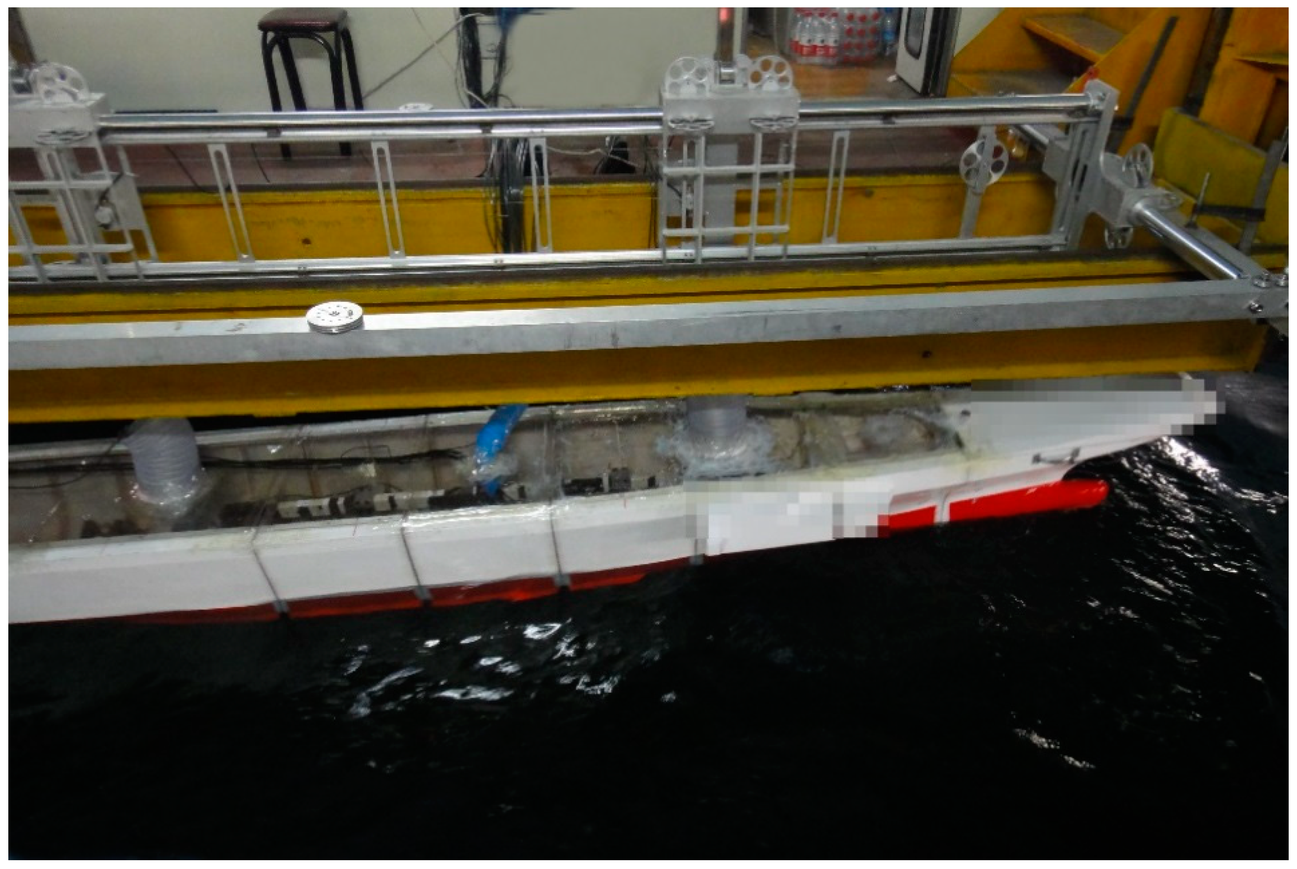
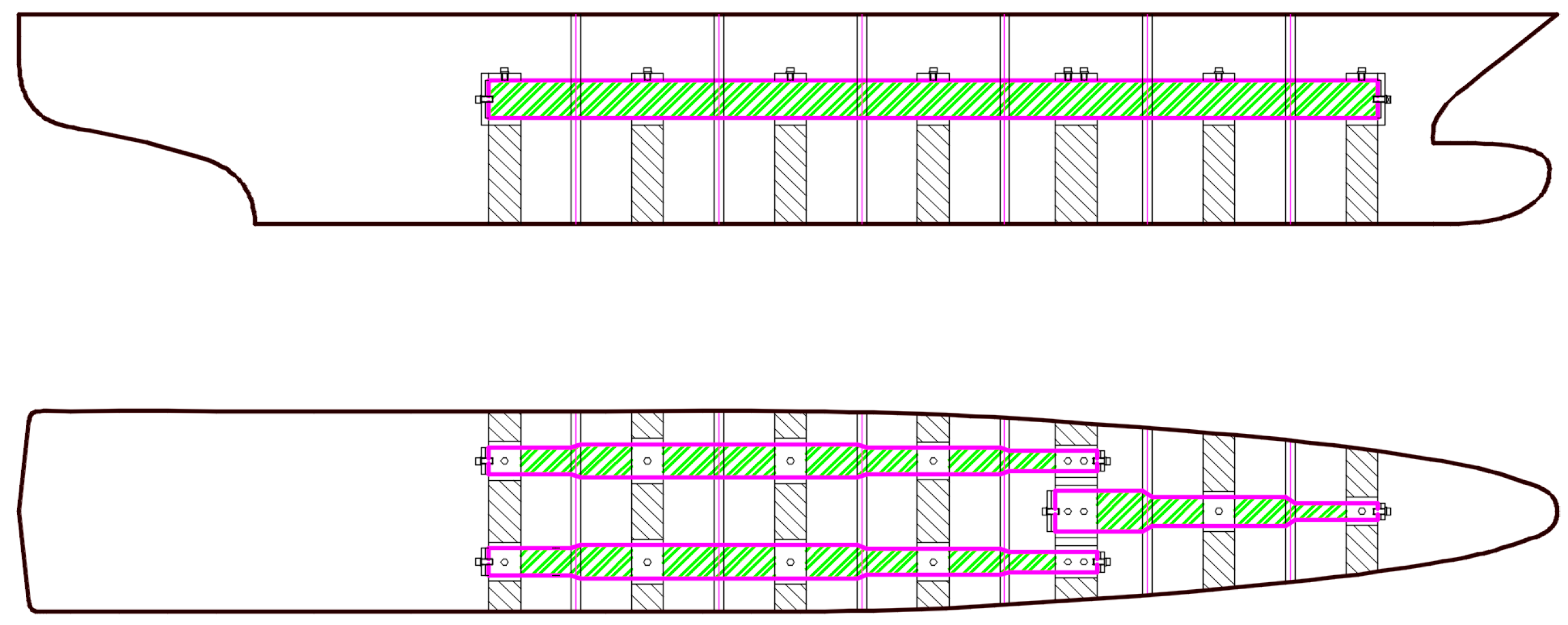
A self-propelled segmented model was designed and manufactured according to the target full-scale ship with broad bow flare.

Table 1. Main particulars of the model.

Scale	1:64
Displacement (kg)	195
Length waterline (m)	4.30
Length overall (m)	4.85
Breadth (m)	0.51
Designed Draft (m)	0.12

presents the principal particulars of the ship model. Figure 2 shows the overview of the segmented model. The elastic model is divided into seven segments longitudinally, and sectional loads at the six cut sections are measured during experiments. A total of three steel backbones are used to connect the segments. The backbones are also made of Q235 steel, and therefore, have the same material parameters as those of the real ship hull beam. The heights and widths of these three steel backbones are iteratively adjusted to fulfil the requirements of the principle of similarity on the flexible characteristics for the purpose of reproducing the hydroelastic effect of the real ship. The first order natural frequency of vertical vibration of the ship model after the iteration process mentioned above is adjusted to be similar with that of the real ship. Figure 3 presents the arrangement of the three backbones. The three steel beams are fitted with strain gauges of 200 Hz sampling rate to measure the M_BV of the model at the cut sections. A propelling system, positioned at the stern region, is designed to reach the expected speed of the model in still water and waves.

The tests were carried out in the ship model towing tank of Harbin Engineering University. The towing tank is 108 m long, 7 m wide, and 3.5 m deep. A towing carriage is used to serve as the platform where the monitoring apparatus such as the data acquisition system are placed. A computer controlled hydraulic driven wave generator, which is currently utilized as flap type, can generate both regular and irregular waves. The waves will be absorbed by a damping beach opposite to the wave maker to prevent the effects of reflected waves on the generated incident waves and the ship model. A wave probe is positioned near the wave generator to monitor and record the generated waves at 50 Hz sampling rate.

Table 2. Capacities of the towing tank.

Parameters	Capacity
Carriage speed (m/s)	0.1~6.0
Wave period (s)	0.4~4.0
Wave natural circular frequency (rad/s)	1.57~15.70
Wave length (m)	0.25~24.99
Maximum regular wave height (m)	0.4
Maximum irregular significant wave height (m)	0.32

gives the main parameters of the towing tank. Figure 4 shows the towing tank and the wave generator.

Wave-induced heave and pitch motions of the model are monitored by an in-house designed, four-freedom motion recorder apparatus, which is installed on the towing carriage and connected to the ship model via two heave rods (see Figure 2). The two heave rods are jointly used to measure heave and pitch motions of the ship model while confine sway and yaw motions. The heave of the ship model at its CG can be derived by the two measured heave values at designated positions where the heave rods are installed. The pitch of the ship model is monitored by the inclinometer, which is fixed on the bottom of the heave rod. The sampling rate of motion is set to be 50 Hz during the experiment.

4. Analysis of Numerical and Experimental Results

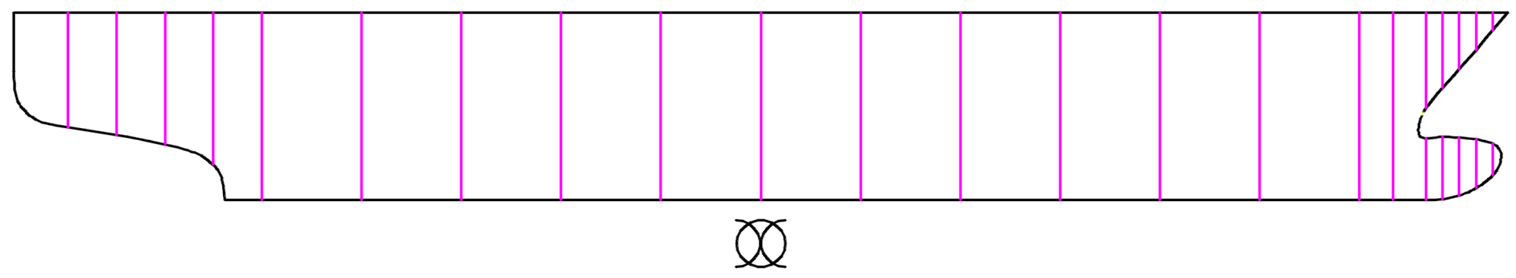
The experimental results and the numerical results are compared and analyzed in this section. For the structural part, the ship structure is modeled by 20 beam elements and the first three elastic modes of vertical bending are used for the solution of structural response. For the hydrodynamic part, a total of 2380 panels are generated by dividing the whole ship hull surface for the computation of nonlinear [F_I] and [F_H]. To calculate the linear [F_R] and [F_D], the wet contact surface of the hull in still water is divided into 2256 panels. Nonlinear [F_SL] is computed based on 22 unevenly-distributed cross sections. Several experimental conditions are selected for the comparison and analysis in this paper, which are listed in

Table 3. Experimental conditions extracted for analysis.

Wave Conditions	Vessel Speed V (kn)	Wave Height H (m)	Wave Period T (s)
Regular wave condition 1	18	4.8	13.28
Regular wave condition 2	18	9.6	13.28
Wave Conditions	Vessel Speed V (kn)	Significant Wave Height H1/3 (m)	Characteristic Wave Period Tz (s)
Irregular wave condition 1	5	18.5	12.5
Irregular wave condition 2	18	9.185	11.5

. Note that the two regular wave periods presented in Table 3 correspond to the relation of λ⁄L = 1.0, where λ and L respectively denote the wave length and the length waterline of the ship. Figure 5 demonstrates the total panels of the whole ship surface and the partial panels under the calm water surface. Figure 6 presents the extracted cross sections along the hull for slamming loads estimation.

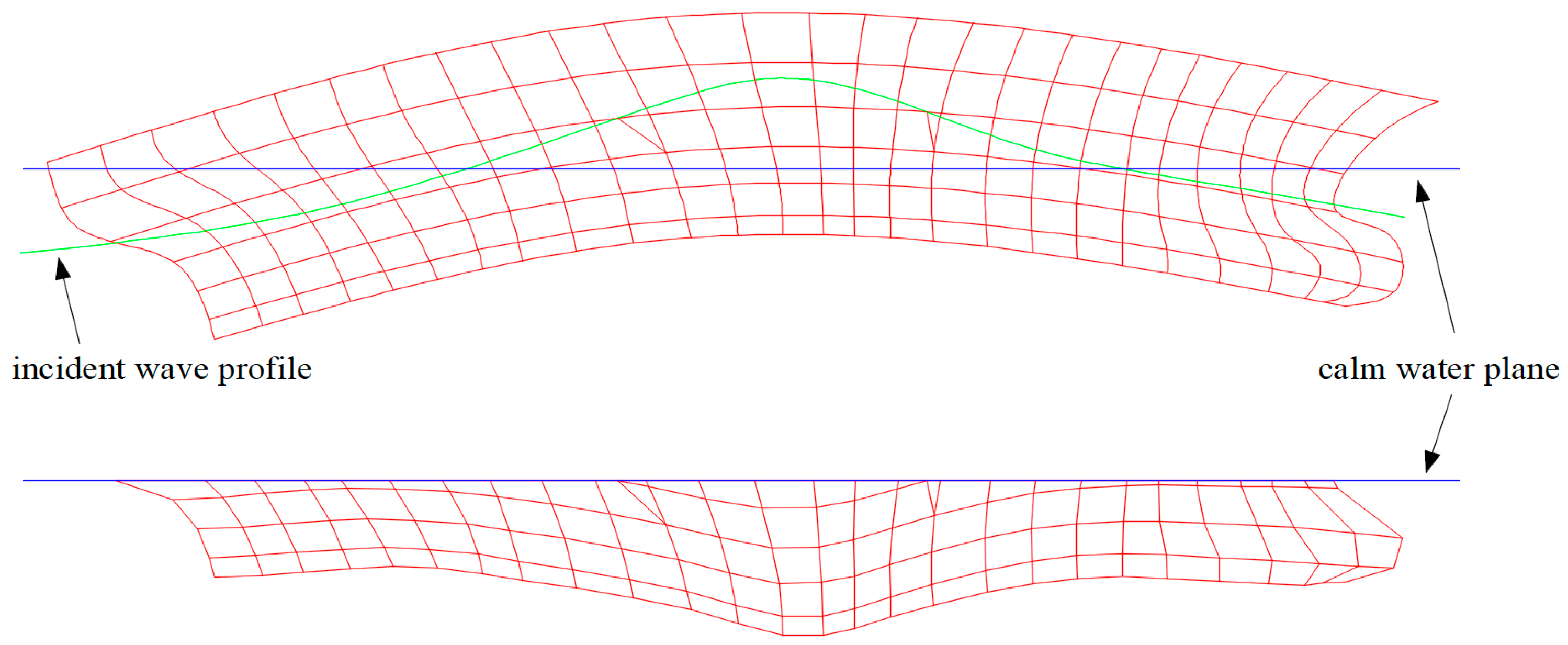
The calculation of nonlinear [F_I] and [F_H], as introduced in Section 2.3, is based on the instantaneous wetted hull surface, the acquisition of which can be accomplished by two steps, as illustrated in Figure 7. The first step is to obtain the so-called physical instantaneous wetted surface by intersecting the deformed ship hull panel with the incident wave profile; see the upper part of Figure 7. In this step, special care should be given to those panels whose vertices are neither all below nor all above the incident wave profile. For panels of this kind, the two intersection points between the incident wave profile and the panel sides are joined together by a straight line segment. If the remaining panel is neither a triangle nor a rectangle, then it is further subdivided into a triangle panel and a rectangle panel. After this first step, a satisfactory physical instantaneous wetted surface is acquired because the difference between the straight line segment and the wave profile within the panel is very small. Note that in Equation (6), the boundary of the free surface is actually the calm waterplane; therefore, the physical instantaneous wetted surface obtained by the first step should be mapped to ensure that the clam waterplane is the boundary of the transformed instantaneous wetted surface [33]. Therefore, the second step is the mapping of the physical instantaneous wetted surface, as shown in the lower part of Figure 7, and the mapped instantaneous wetted surface will be adopted.

Different from [F_I] and [F_H], [F_D] and [F_R] are actually linear and computed based on the mean wetted ship hull surface. In principle, [F_D] and [F_R] are also nonlinear, since [F_I] and [F_H] are nonlinear for the case of ship hydroelastic responses in large waves, and therefore, should also be calculated on the instantaneous wetted surface. However, the re-panelization of the deformed ship hull at each time step, as introduced in the last paragraph, requires the corresponding re-computation of Green function and the subsequent radiation and diffraction wave potentials as determined in Equation (6), thus considerably increasing the computing time, and significantly restricting the application of the presented method in shipbuilding industry. In the present research, we do not consider the nonlinearities of [F_D] and [F_R] associated with the change of the actual wetted ship hull geometry.

Before we proceed to present the experimental and numerical results in the following sections, we briefly discuss the effect of the tank side walls. Compared with the real ship sailing in open seas, the ship model may be affected by the reflected waves from both tank side walls during the experiments. The International Towing Tank Conference (ITTC) released guidelines [34] to avoid such interference from the tank side walls in head waves. Based on the guidelines, the two regular wave conditions are free from the tank side wall effects. However, the effect of the side walls is unavoidable for irregular wave conditions because the irregular wave inevitably contains those regular wave components which will induce the side wall effect. To minimize the side wall effect, the first irregular wave condition in the present research has a rather large significant wave height, resulting in severe slamming events and subsequent wave breaking and large eddies that will greatly dissipate the energy of scattered waves. For the second irregular wave condition, only very few regular wave components may cause the side wall effect due to the relatively high vessel speed. In addition, the relatively high ship speed will also give rise to frequent slamming events that will significantly reduce the side wall effect by the energy dissipation mechanism. Therefore, the tank side wall effect in the present study is significantly reduced, and the experimental results are trustable.

4.1. Necessary Hydrodynamic Results

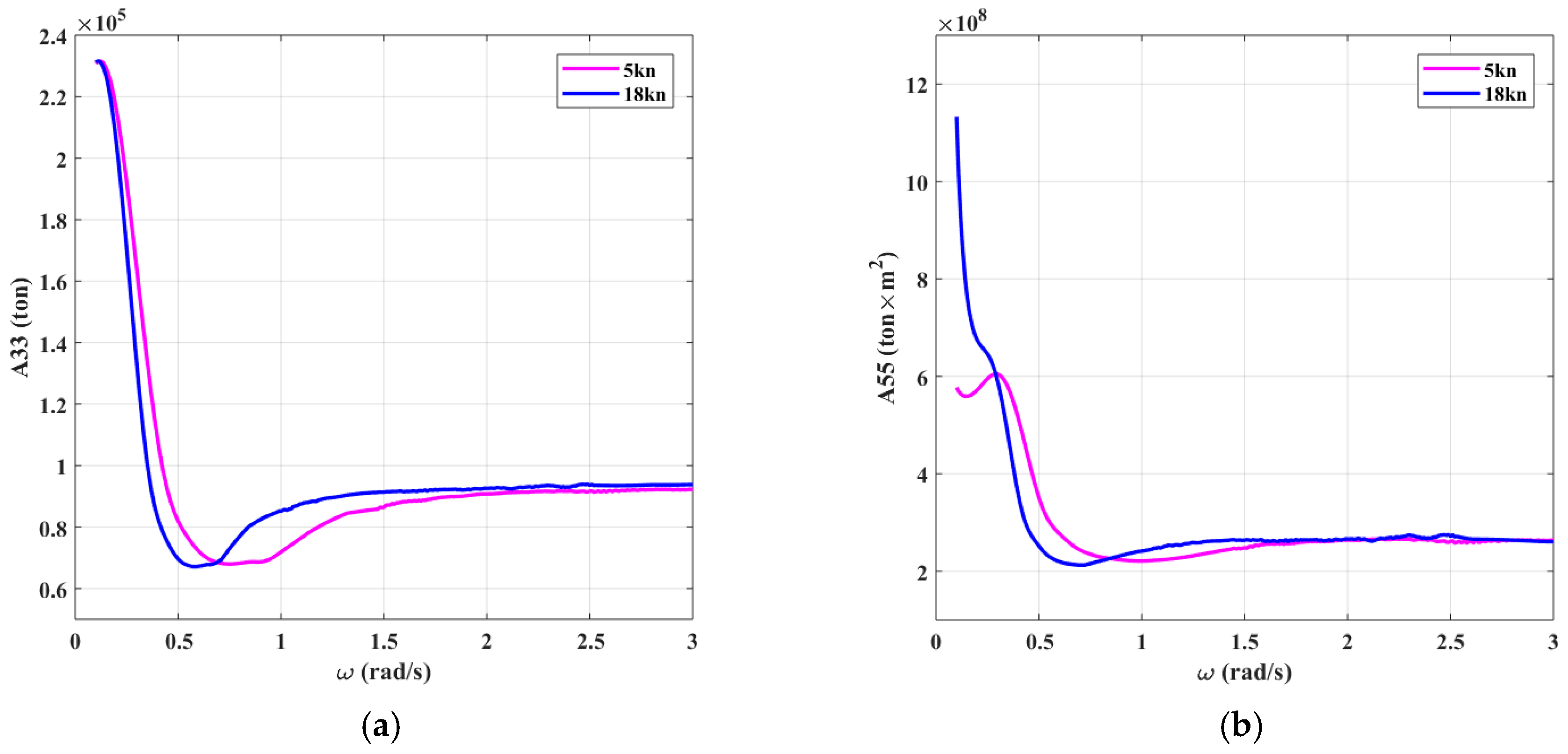
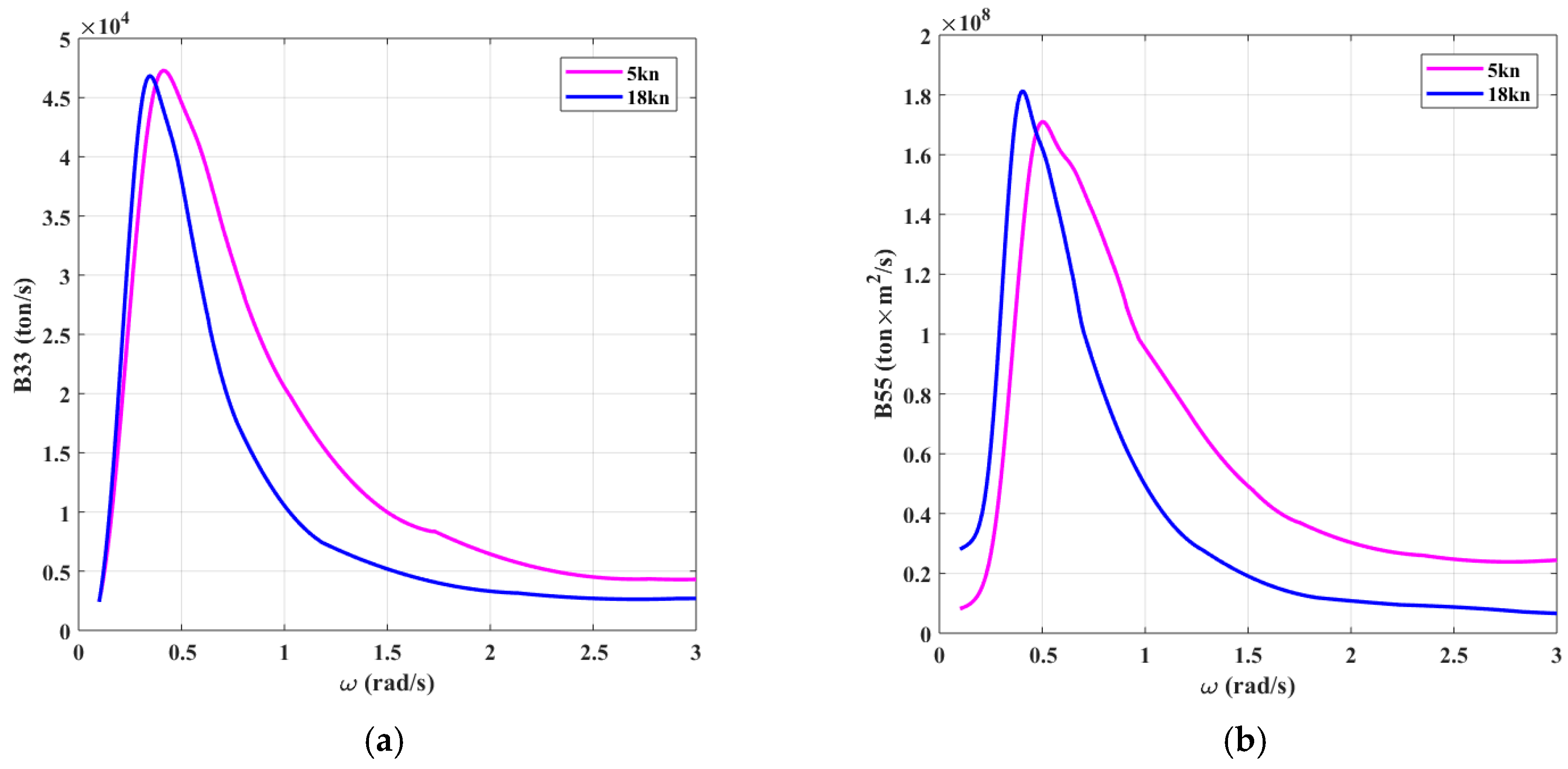
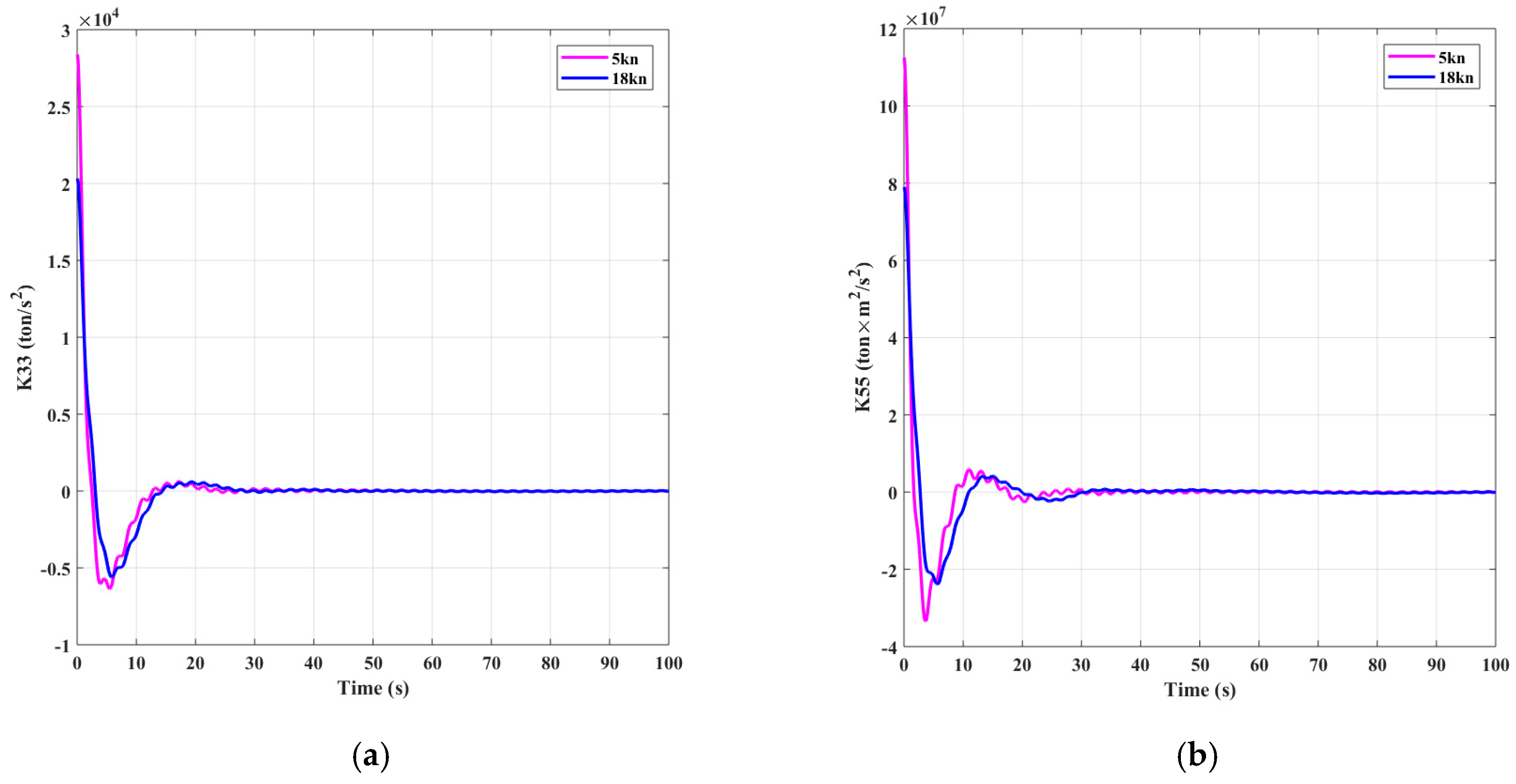
In this section, hydrodynamic coefficients and retardation functions obtained by the hydroelastic code are presented and analyzed. The added masses of A₃₃ and A₅₅, damping coefficients of B₃₃ and B₅₅, and the retardation functions of K₃₃ and K₅₅ of the target ship with forward speeds 5 kn and 18 kn in head regular waves are presented in Figure 8, Figure 9 and Figure 10. As can be seen from Figure 8, both A₃₃ and A₅₅ vary significantly with respect to the natural circular frequency ω of the incident wave when ω is less than 0.5 rad/s. For ω greater than 1.5 rad/s, these two added mass coefficients change very slightly. Different from A₃₃, ship velocity plays a more vital role in A₅₅ when ω is less than 0.3 rad/s. As velocity increases from 5 kn to 18kn, positions of occurrence of the peak values in B₃₃ and B₅₅ both move leftward a little bit, with the peak value of B₃₃ changing less significantly than that of B₅₅. Similar to A₃₃ and A₅₅, the variations of B₃₃ and B₅₅ with respect to ω are much more evident when ω falls in the interval of 0.1 rad/s to 1.5 rad/s. The general shapes of retardation functions K₃₃ and K₅₅ are similar, and small oscillations can be found in these two curves. Both K₃₃ and K₅₅ decay quickly with respect to time, as can be observed in Figure 10.

4.2. Modal Analysis

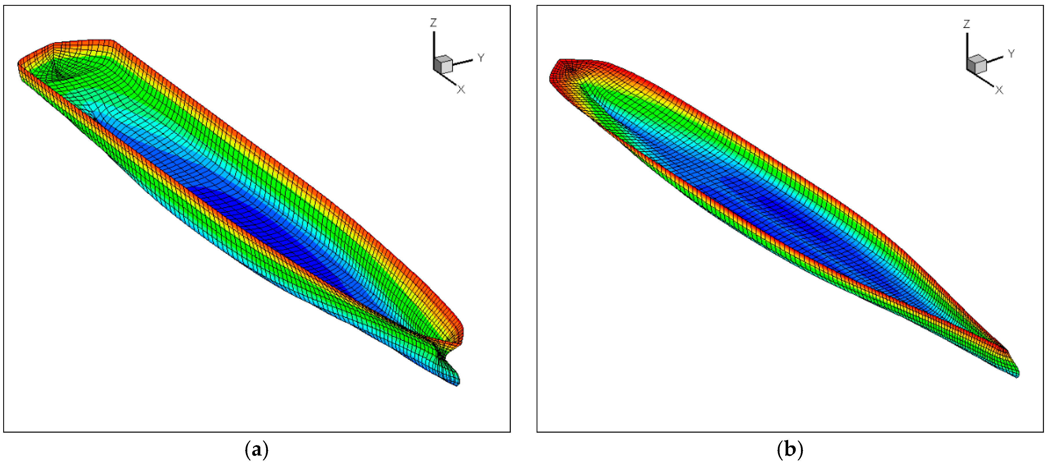
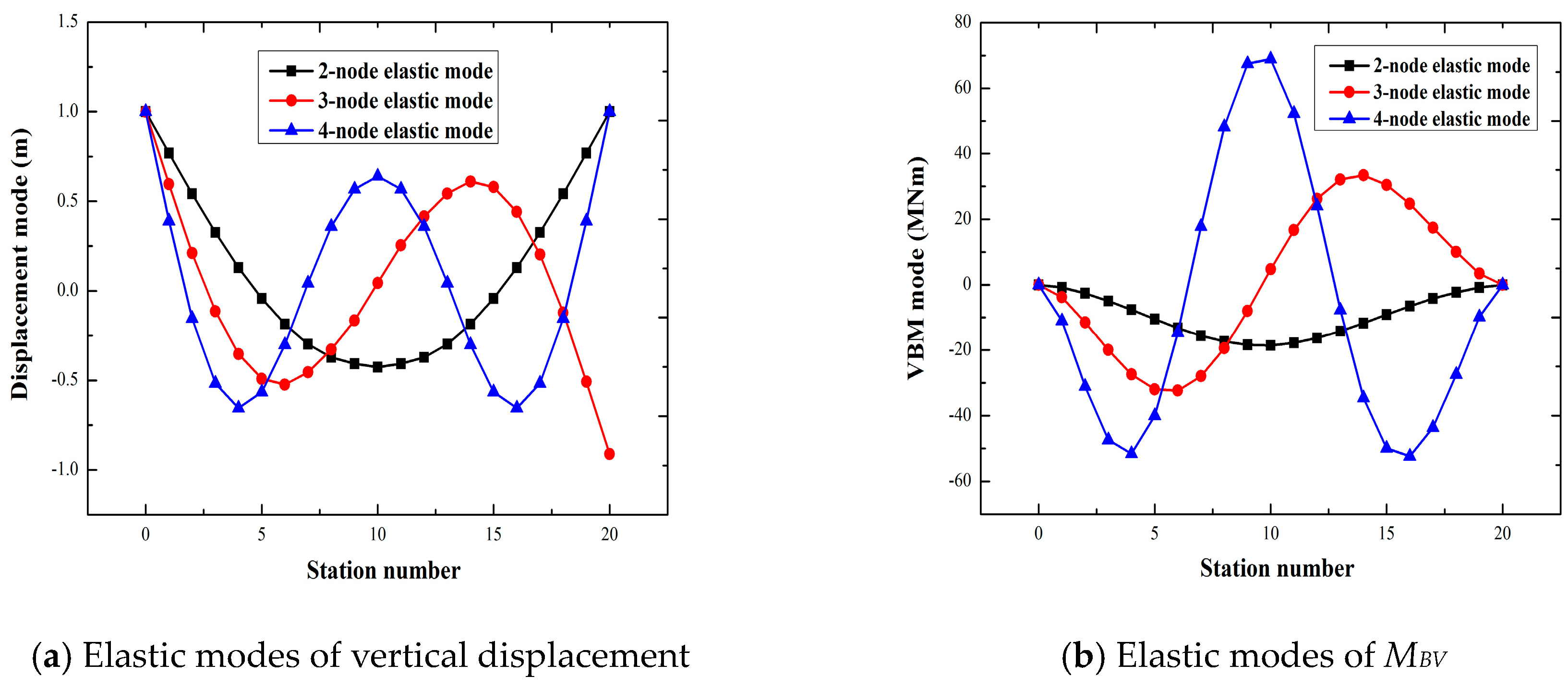
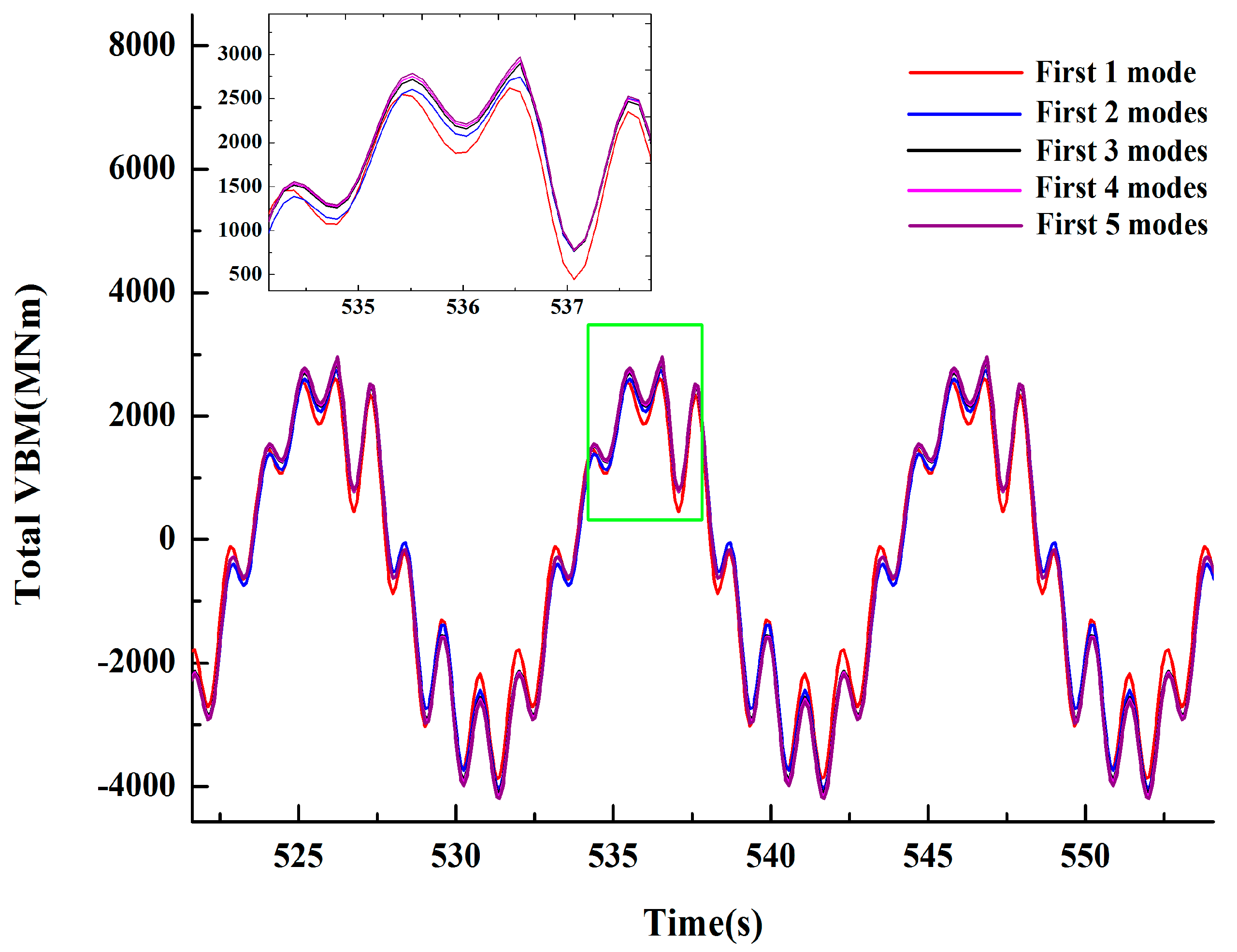
Based on the Timoshenko beam theory and the transfer matrix method, the first three vertical vibrational elastic modes are numerically obtained; see Figure 11. Based on the conclusions of [35,36], in the present research we do not give the experimental elastic vertical modes. A hammering test of the experimental model was carried out in calm water to validate the numerical result. The natural frequencies can be obtained by Fourier transform of the decayed time series of the transient structural response following the hammering impact.

Table 4. Comparison of wet natural frequencies.

Order of Mode	Numerical Results (Hz)	Experimental Results (Hz)	Relative Error (%)
First	0.752	0.727	3.439
Second	1.531	1.703	−10.100
Third	2.151	2.679	−19.709

presents the comparison of elastic vibrational wetted natural frequencies between calculation and measurement. The discrepancy between the experimental and numerical results for the wet natural frequency of the first order is 3.439%, which satisfied quite well the requirement of the principle of similarity. Although the errors for the second and third orders of wet natural frequencies are larger than 10%, they have little influence on the overall results, because the effect of the higher order deformation modes on the loads is rather small compared with the first order vibrational mode, which can be verified by Figure 12. In Figure 12, the vertical bending moments obtained based on different number of elastic vibrational modes are presented; it can be concluded that the first order deformation mode is most important, and the contributions from orders of elastic modes greater than three can be safely discarded. A similar conclusion for a linear case was also reported in [37].

4.3. Hydroelastic Responses in Regular Waves

4.3.1. Analysis of Experimental Regular Waves

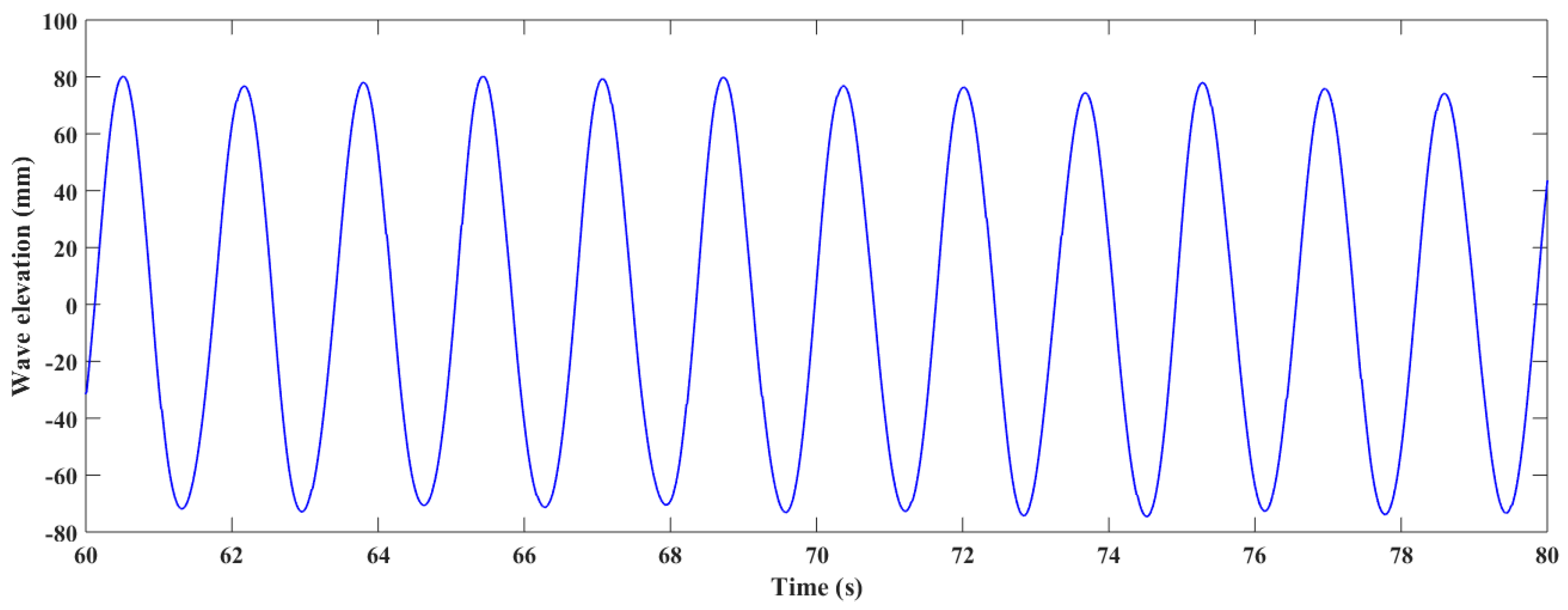
The experimental regular waves are generated by the flap type wave maker, and a wave probe was positioned near the wave generator to monitor the waves. Figure 13 illustrates the time history of the experimentally-generated regular wave with the theoretical wave height and wave period being 150 mm and 1.66 s at model scale, respectively. A total of 12 periods are shown in Figure 13, and each wave peak (or wave trough) slightly differs from each other due to the inevitable uncertainty associated with the experimental flap type wave maker. The relatively smooth region of the shown time history is extracted to calculate the mean actual wave height and wave period generated, and the comparison of experimental results and expected values are shown in

Table 5. Comparison of regular wave characteristics at model scale.

	Condition 1 (4.8 m, 13.28 s)			Condition 2 (9.6 m, 13.28 s)
	Experiment	Target	Error (%)	Experiment	Target	Error (%)
Wave height (mm)	76.36	75.0	1.81	150.09	150.0	0.06
Wave period (s)	1.65	1.66	−0.6	1.65	1.66	−0.6

. The two regular, experimentally-generated wave conditions are in good agreement with the input regular wave parameters on average, with the biggest relative error of the wave height being 1.81%.

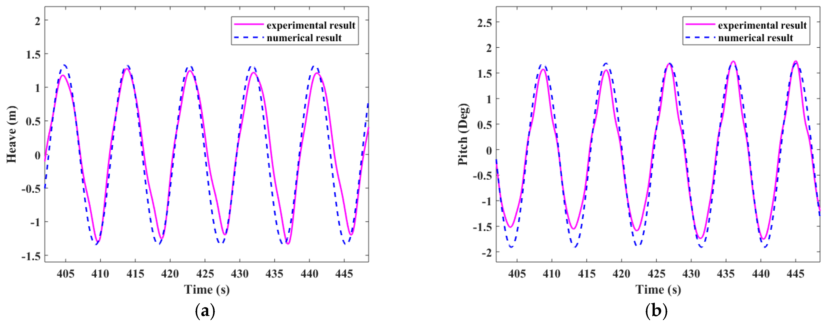
4.3.2. Motions in Regular Waves

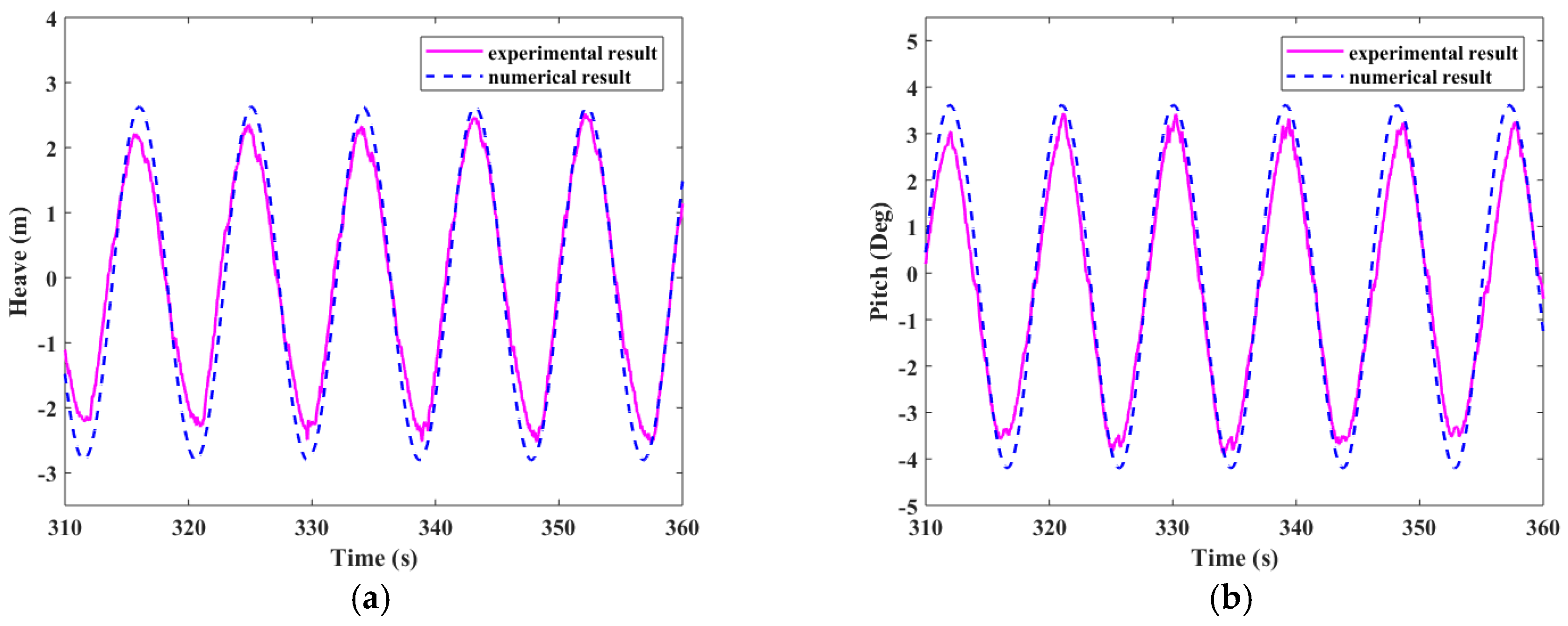
The experimental and numerical hydroelastic responses of heave and pitch at CG of the target ship are extracted and analyzed for the two regular wave conditions. Figure 14 and Figure 15 display the comparison of motion responses in the two testing conditions. The experimental heave and pitch responses show some oscillations in both peaks and troughs compared with the numerical results. This is because the phenomenon of forward speed fluctuation of ships in waves can naturally occur in the present self-propelled ship model experiment, while the present numerical method assumes that the ship velocity remains unchanged during the whole simulation process. In addition, since the experimentally-generated wave peaks (or wave troughs) slightly differ from each other as illustrated in Figure 13, the ship model motion responses under such experimental waves will consequently show some difference in their peak values and trough values, as demonstrated in Figure 14 and Figure 15. The numerical results slightly overestimate the heave and pitch responses on average compared with the experimental results, as can be found in Figure 14 and Figure 15, probably due to the omission of dissipation effects associated with fluid viscosity in the current numerical methodology. Figure 14a and Figure 15a show that, on average, the peak values and trough values of heave response are nearly symmetric. In comparison, both the experimental and numerical trough values of pitch response are larger than peak values. This phenomenon results from the joint effect of nonlinearity of the ship hull geometry and the dynamic effect of waves. Here, negative pitch values represent the trim by stern, meaning that in the present case the specific ship hull geometry tends to lift the ship bow region a little bit in waves. The experimental results of both heave and pitch responses include some minor noise due to the friction and vibration of the motion monitor apparatus. In general, the numerical results agree satisfactorily with the experimental results.

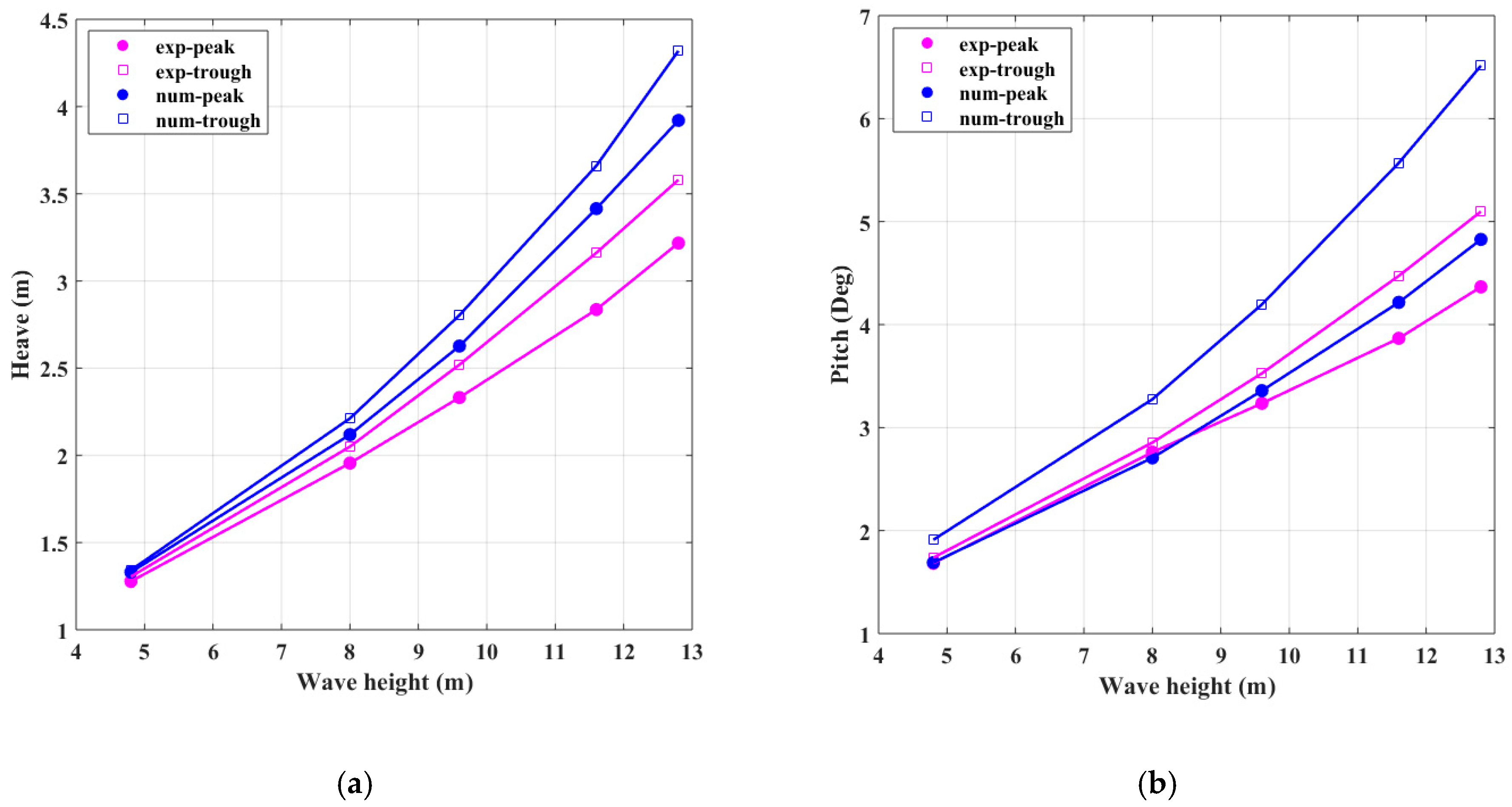
The results of peaks and troughs of motion responses at different wave heights with forward speed 18kn are demonstrated in Figure 16. As the wave height increases, both the peaks and troughs of the heave and pitch responses increase nonlinearly, with the degree of overestimation of numerical results increasing accordingly. Compared with the peaks of motion responses, the nonlinear effect manifested by the troughs of motion responses is more evident. Figure 16 also shows that, with the increase of wave heights, the asymmetry of peaks and troughs in both heave and pitch responses increases. The asymmetry of peaks and troughs in pitch motion becomes increasingly larger than that in heave motion as the wave height continues to increase.

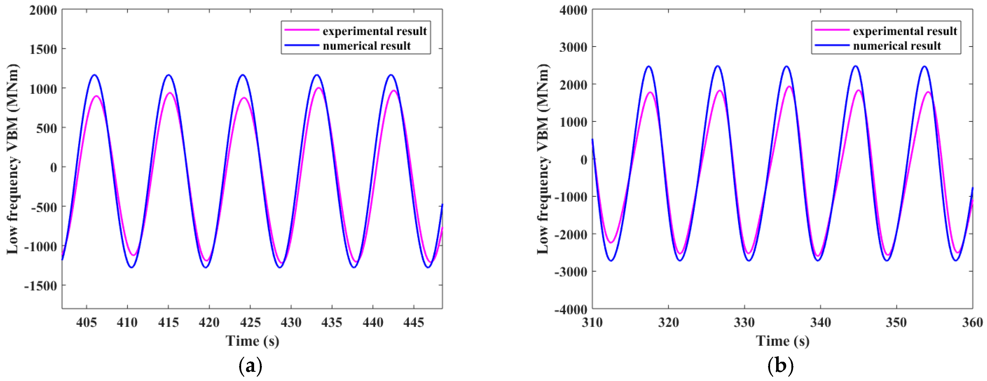
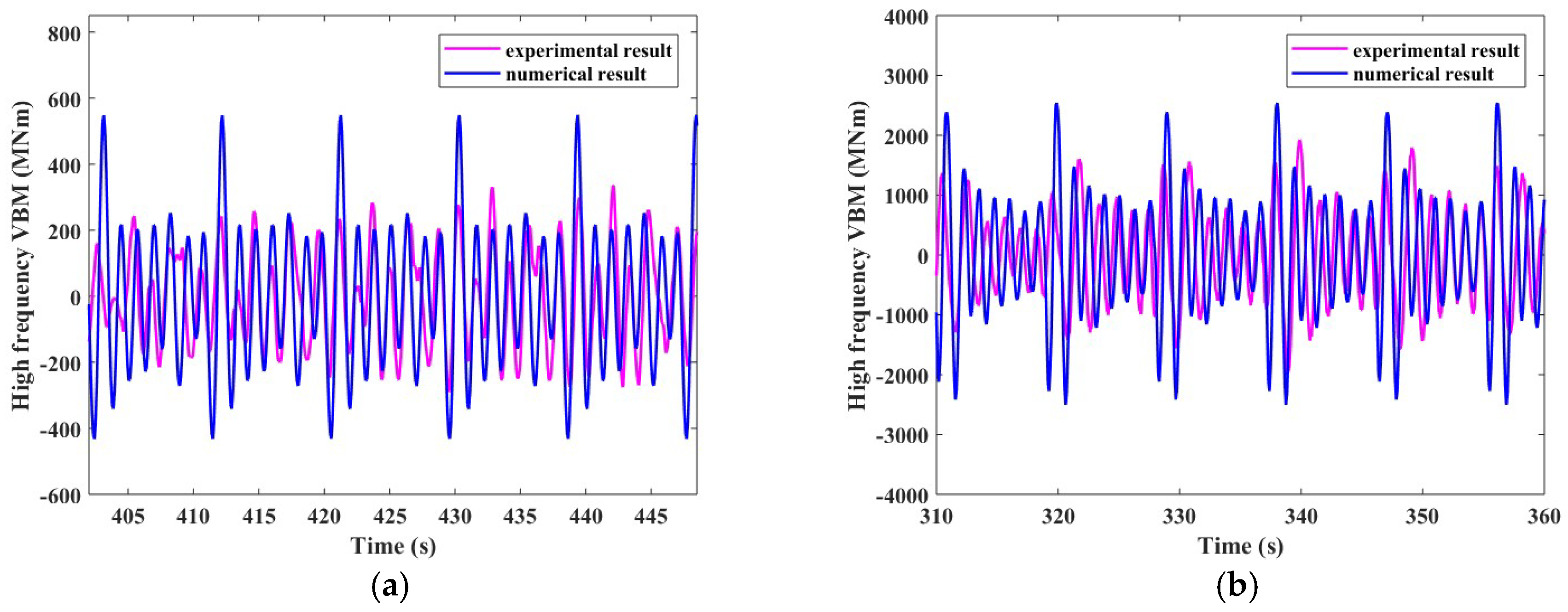
4.3.3. M_BV in Regular Waves

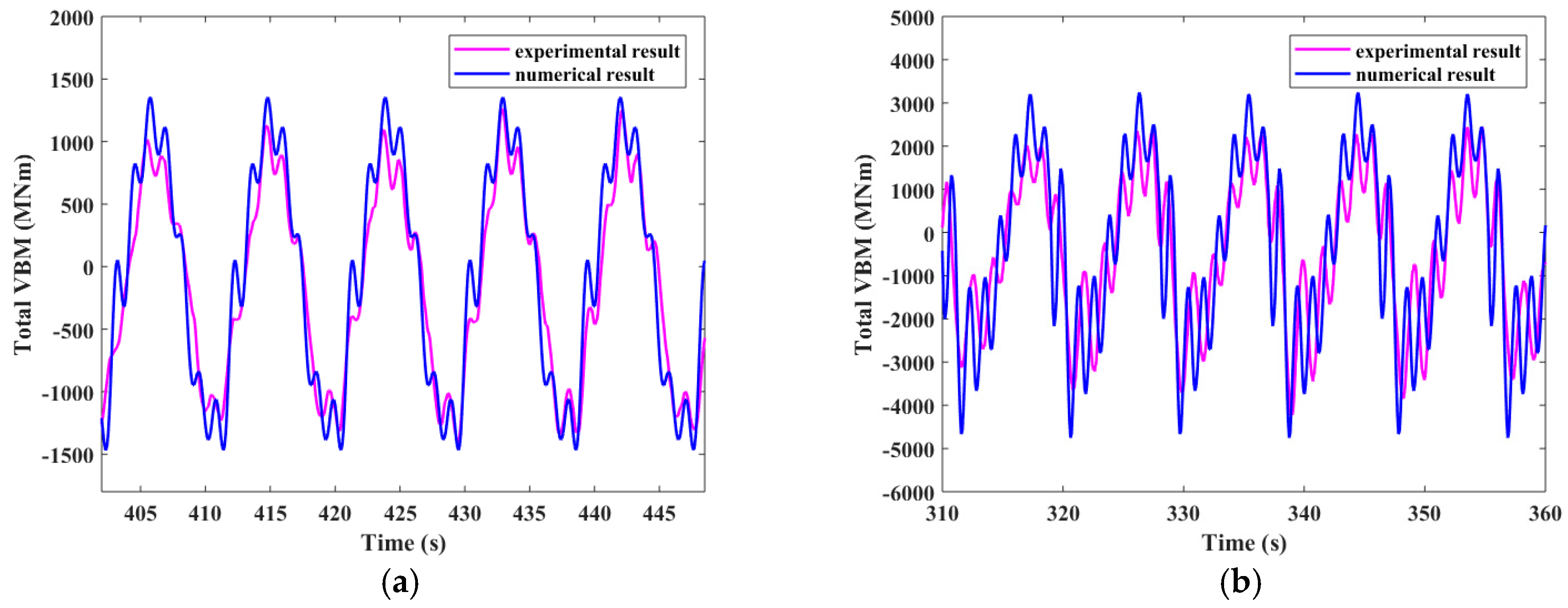
Together with the extraction and analysis of motion responses, experimental M_BVs amidships of the target ship in the two regular wave conditions are also compared and analyzed with numerically obtained M_BVs. The total M_BVs are decomposed into low frequency and high frequency components corresponding to forced vibration excited by the regular incident waves and slammed vibration due to wave impact, as presented in Figure 17, Figure 18 and Figure 19. On average, the numerical total M_BVs, low frequency M_BVs and high frequency slamming M_BVs agree satisfactorily with the experimental counterparts. Similar to the motion responses in Figure 14 and Figure 15, the M_BVs predicted by the numerical method are slightly larger than the results obtained experimentally. The ship model velocity fluctuation and the oscillations of the extrema of the generated waves during the experiment also contribute to the oscillations of hogging and sagging values of both the total M_BVs and the component loads. Compared with the experimental results, the present numerical method can also produce asymmetrical peaks and troughs of the total and low frequency M_BVs responses resulted from the nonlinearity associated with the ship hull geometry. Figure 18 shows that the experimental and numerical low frequency sagging M_BVs agree pretty satisfactorily, with some discrepancies being found between numerical and experimental hogging M_BVs which are due to the limited nonlinear factors considered in the numerical method. The peak values of numerical high frequency slamming M_BVs are also overestimated compared with the experimental results; see Figure 19.

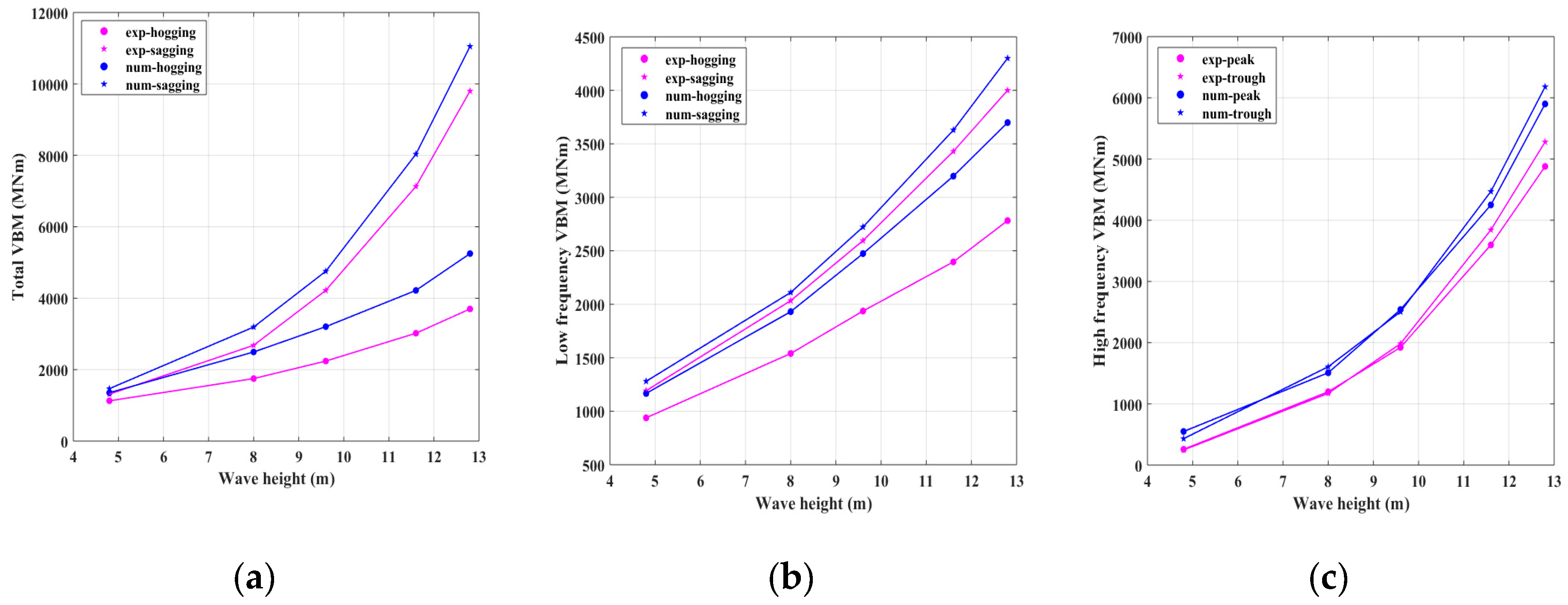
Figure 20 shows the relationship of hogging and sagging values of M_BVs with respect to wave heights at the ship speed of 18 kn. As can be seen clearly from Figure 20, the total M_BVs, low frequency M_BVs and high frequency slamming M_BVs all vary nonlinearly with the increase of the wave height. Compared with the hogging and sagging values of the total M_BVs and low frequency M_BVs, the magnitudes of peaks and troughs of the high frequency slamming M_BVs are much closer; see Figure 20c. The evident difference between the absolute values of the hogging and sagging M_BVs for the total M_BVs and low frequency M_BVs is mainly due to the nonlinear effect of the change of wet hull geometry on which the wave pressure acts for a relatively long duration in every incident wave period. In comparison, the high frequency slamming M_BVs are caused by transient local wave impact, meaning that during the very short duration of whipping, the change of the wetted hull surface is negligible, and therefore, the above-mentioned effects play little role in the asymmetric characteristics of hogging and sagging M_BVs of the high frequency M_BVs. The omission of some strong nonlinear effects in extreme waves from the present numerical method, such as wave breaking, large eddies, large ship motions, etc., results in the evident discrepancy between the numerical and experimental results in large to extreme waves. Wave breaking and large eddies generated by water viscosity in experiments will dissipate the energy of the ship model system, leading to mitigated ship model responses. The tank side wall effect may also slightly contribute to the difference between the numerical predictions and the experimental results, since this effect is not considered in the present numerical model. On the other hand, large ship motions in extreme waves indicate that not only the [F_I] and [F_H], but [F_D] and [F_R] should be calculated based on the 3D instantaneous wetted ship hull, which is currently still a challenge in potential flow approach. The present numerical methodology can reasonably predict the hydroelastic responses in large to extreme waves, even though some discrepancies can be found. Compared with the low frequency M_BVs, the hogging and sagging values of the total M_BVs and high frequency slamming M_BVs change more rapidly as the wave height increases. This is because the transient high frequency impact M_BVs are more sensitive to the local change of the wave impact pressure resulted from the increase of incident wave height. Since the high frequency M_BVs constitute an important part of the total M_BVs, the total M_BVs accordingly change rapidly with the increase of wave heights.

4.4. Hydroelastic Responses in Irregular Waves

4.4.1. The Irregular Waves

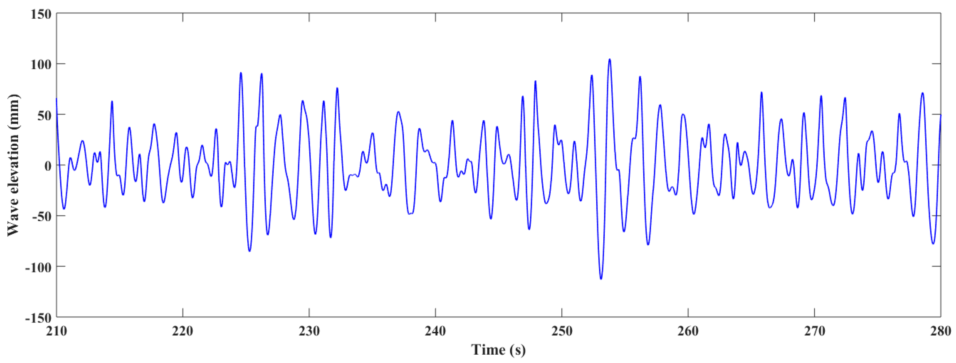
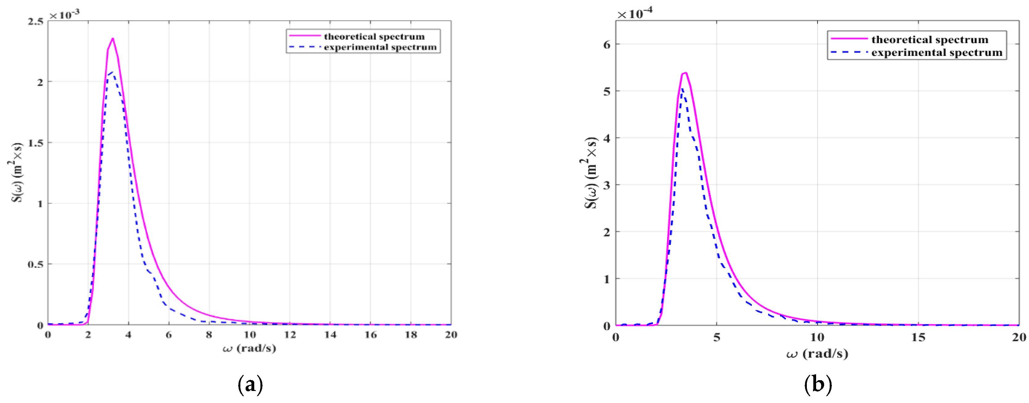
The results in the two typical irregular wave conditions are analyzed in this section. The irregular waves are simulated according to the ISSC spectrum using the expected parameters in

Table 6. Comparison of irregular wave parameters at model scale.

	Condition 1 (H1/3 = 18.5 m, Tz = 12.5 s)			Condition 2 (H1/3 = 9.185 m, Tz = 11.5 s)
	Experiment	Target	Error (%)	Experiment	Target	Error (%)
Significant wave height H1/3 (mm)	277.504	289.063	−4.0	139.891	143.516	−2.53
Characteristic wave period Tz (s)	1.609	1.563	2.94	1.413	1.438	−1.75

. An example of time series recorded by the wave probe during experiment is shown in Figure 21. Then, the experimental wave spectrum can be obtained by correlation function method using the measured time series. A comparison of the wave spectra between the experimental and target results is shown in Figure 22. The comparison indicates that the experimental waves generated by the wave maker are in fairly good agreement with the expected waves. Moreover, as seen from Table 6, the parameters, i.e., the significant wave heights and characteristic wave periods, of generated waves are also found to be close to the expected values.

4.4.2. Motions in Irregular Waves

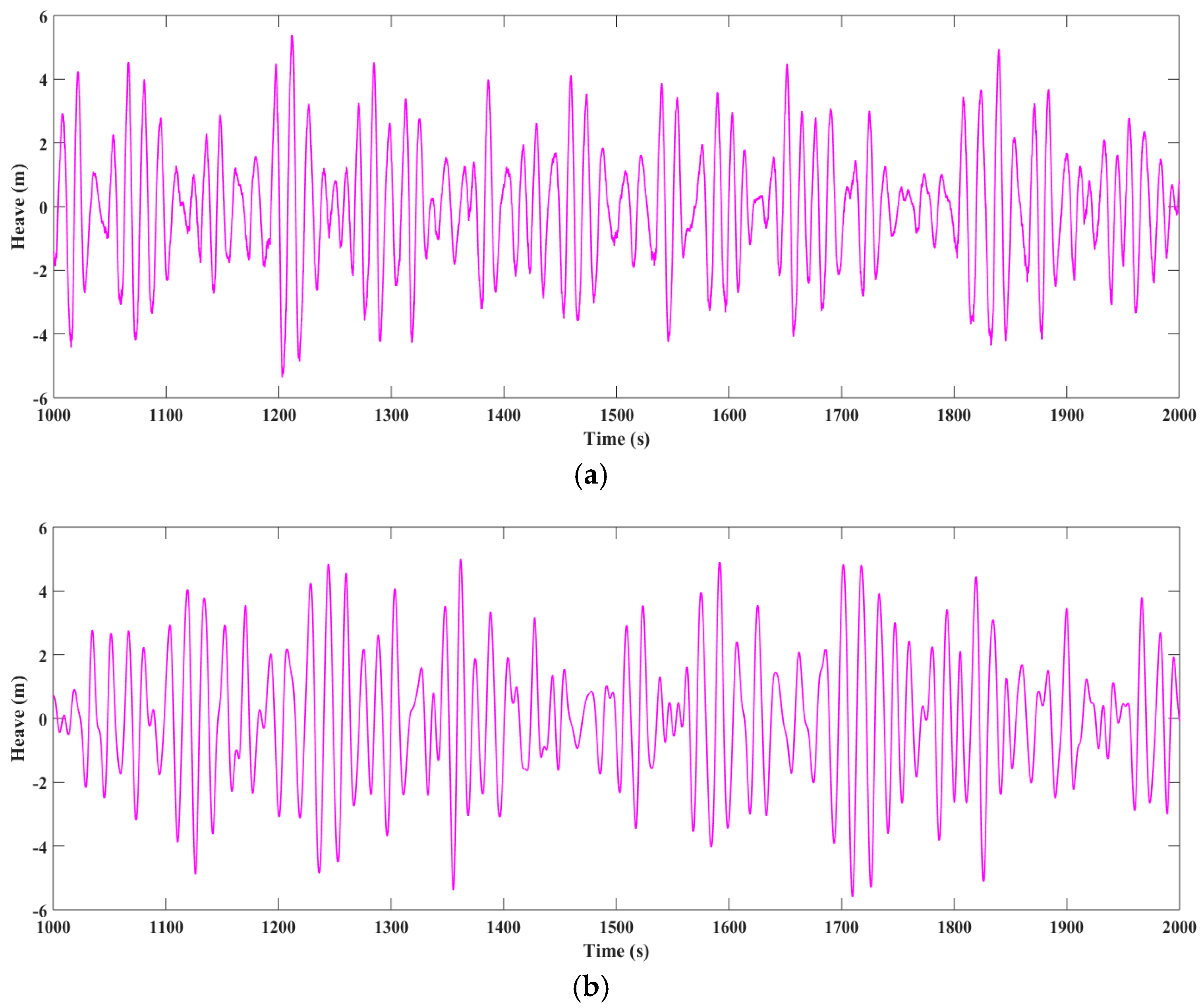
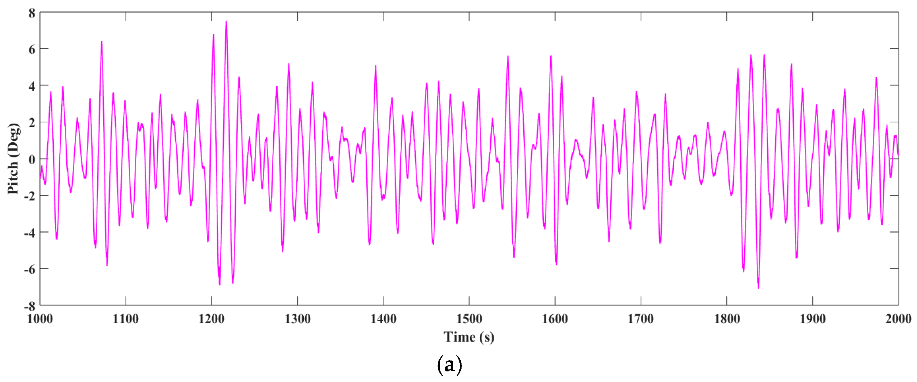
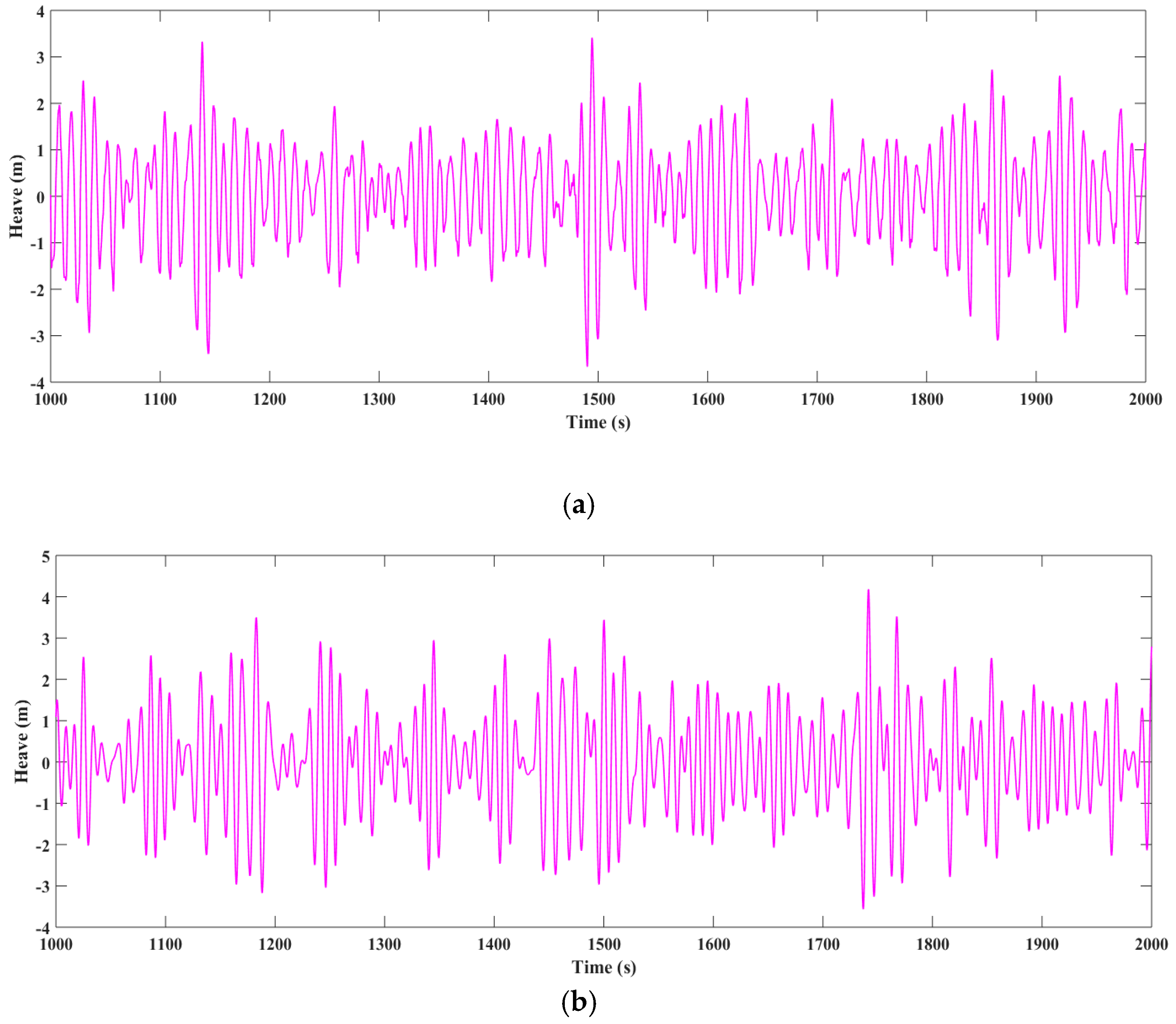
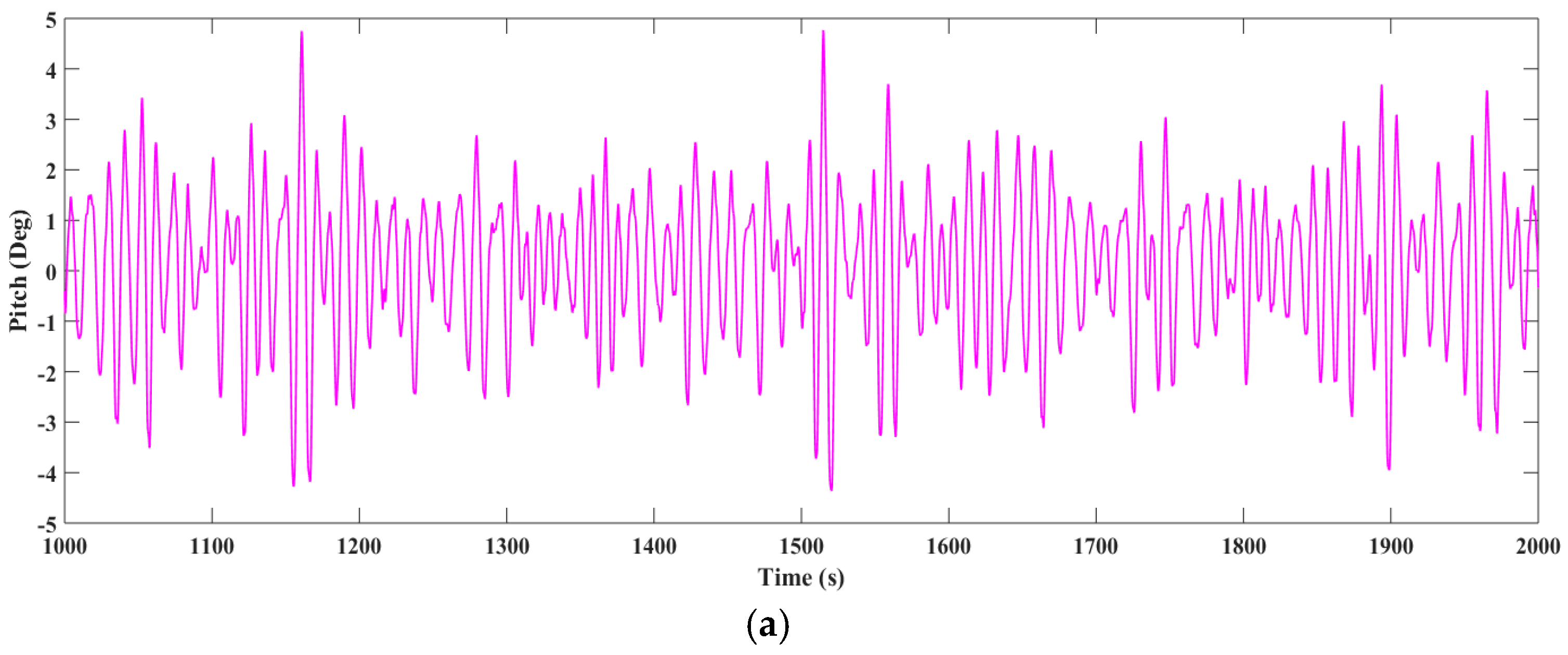
The ship responses during a short-term period of 1 h are simulated by the numerical calculation to obtain enough sample data for the subsequent statistical analysis. Since the length of the towing tank is not long enough for the collection of sufficient experimental sample data in a single run of the ship model, a total of 8 runs of the ship model for each irregular wave condition were conducted. Then, the total time series were obtained by connecting the measured time series of each run in the same sea state, thus providing enough experimental data for the following analysis. The time series of heave and pitch motions at CG of the full-scale ship within 1000 s are qualitatively compared from Figure 23, Figure 24, Figure 25 and Figure 26. Note that in the present research, the experimental and numerical irregular waves are independently randomly generated according to the same target ISSC wave spectra, and thus, the experimental and numerical details of the component regular waves, namely, the wave amplitude and initial wave phase of each component regular wave, may be different because they are inherently probabilistic. The elevation of the irregular waves is, in fact, generated by assigning a random initial wave phase to each regular wave component during the numerical simulation. Since the time series of experimental and numerical irregular waves differ in fine details, the consequent experimental and numerical time series of hydroelastic motion responses will accordingly not agree in fine detail as demonstrated from Figure 23, Figure 24, Figure 25 and Figure 26. In comparison, the experimental and numerical results of heave and pitch responses respectively show similarity in trends and magnitudes, qualitatively verifying the validity of the numerical prediction, but still indicating the need for statistical analysis.

The statistical parameters of the hydroelastic motion responses are adopted to describe the ship responses in short-term irregular waves. The comparison of statistical parameters by measurement and calculation is listed in

Table 7. Statistical parameters of heave and pitch at CG of ship.

Item		Condition 1 (V = 5 kn, H1/3 = 18.5 m, Tz = 12.5 s)			Condition 2 (V = 18 kn, H1/3 = 9.185 m, Tz = 11.5 s)
		Experiment	Calculation	Error	Experiment	Calculation	Error
Heave	Peak significant value (m)	3.59	4.03	12.26%	2.15	2.48	15.35%
	Trough significant value (m)	−3.67	−4.04	10.08%	−2.22	−2.53	13.96%
	Mean value (m)	−0.06	−0.025	————	0.0082	−0.0037	————
	Standard deviation (m)	2.63	2.90	10.27%	1.56	1.75	12.18%
Pitch	Peak significant value (deg)	4.75	5.27	10.95%	2.97	3.47	16.84%
	Trough significant value (deg)	−4.84	−5.32	9.92%	−3.18	-3.51	10.38%
	Mean value (deg)	0.025	−0.00044	————	0.0065	0.00003	————
	Standard deviation (deg)	3.42	3.74	9.36%	2.20	2.49	13.18%

. Note that for both irregular wave conditions, we present the mean values of heave and pitch responses without calculating the relative errors. This is because the experimental mean values of both heave and pitch motions contain inevitable experimental uncertainties mainly associated with the initial experimental conditions. For each run, we have to choose the initial position of the ship model as the balance position relative to which the heave and pitch responses are experimentally measured. The realistic water surface in the towing tank after each run always contains small ripples that slightly move the ship model from its theoretical balance position used in numerical simulation. It is this experimental error that makes the mean values of experimental heave and pitch motions greatly deviate from those obtained numerically. However, since this experimental error is negligibly small compared with other statistical parameters, it is still reasonable to compare other numerical and experimental statistical parameters. The results indicate that good agreement is achieved between experimental and numerical significant values for peaks and troughs of motion responses, with the difference being less than 16.84%. The relative errors for peak and trough significant values of both heave and pitch motions appear to be larger for higher speed condition, probably due to the insufficient consideration of nonlinearities associated with ship velocity in numerical simulation. The standard deviation also shows satisfactory results between experiment and calculation, with relative error being less than 13.18%.

4.4.3. M_BV in Irregular Waves

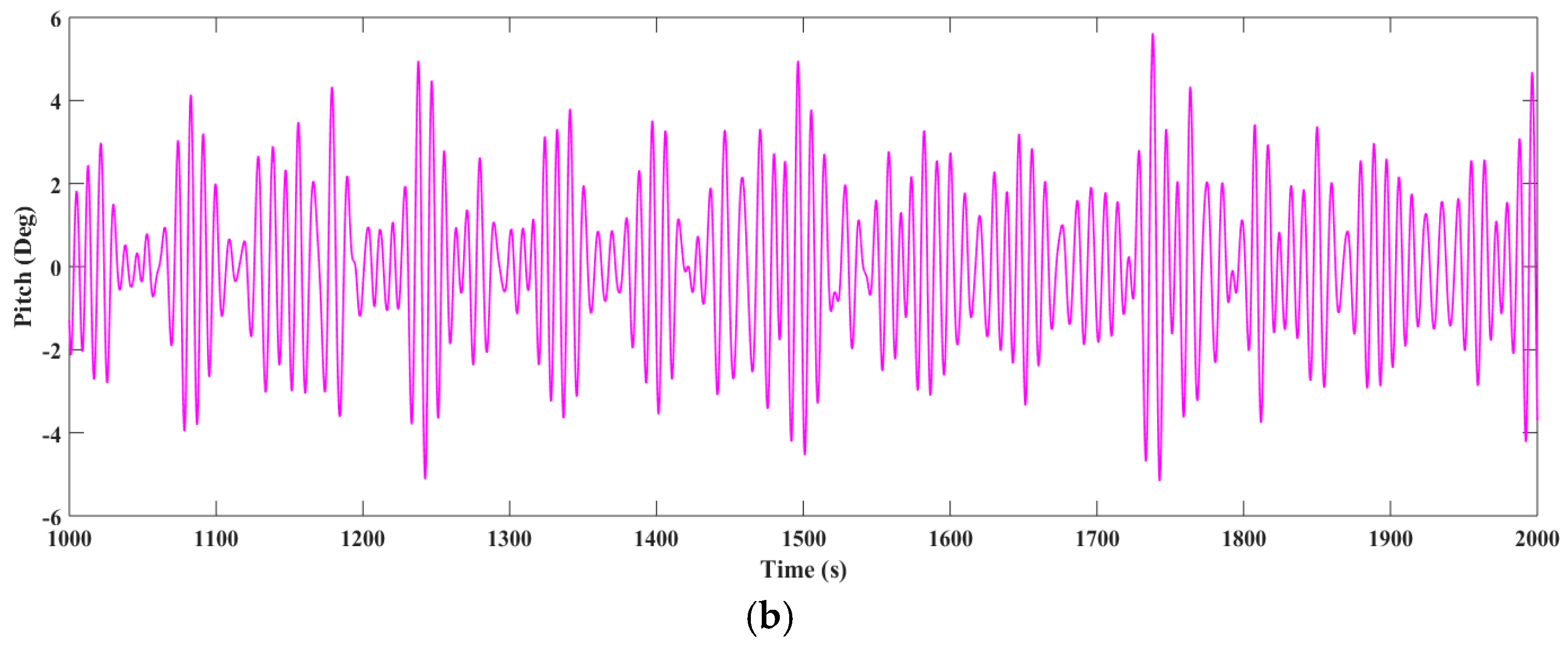
The time series of M_BVs amidships of the full-scale ship within 1100 s are shown in Figure 27 and Figure 28, where the low-frequency components and high-frequency components are also separated from the total M_BVs by Fourier filtering similar to the treatment of M_BVs in regular wave conditions. Similar to the last section, here the experimental and numerical results are also qualitatively compared, and similar magnitudes and trends between calculation and measurement can be found from comparisons of M_BVs. As can be seen, several severe slamming events occurred during ship sailing in irregular waves because of high speed or large wave amplitudes. The slamming M_BVs decay rapidly due to the structural damping if two adjacent slamming events do not occur too closely. In irregular wave testing condition 1, the magnitude of slamming M_BVs is almost the same as that of low frequency M_BVs due to the large wave amplitude of irregular wave condition 1 on average. In comparison, for irregular wave testing condition 2, the magnitude of slamming M_BVs is obviously smaller than that of low frequency M_BVs due to the relatively smaller wave amplitude of irregular wave condition 2 compared with that of irregular wave condition 1. For these two irregular wave conditions, the experimental occurrence frequencies of wave impact manifested by the slamming M_BVs differ slightly, indicating that both large wave amplitude and high ship speed will increase the chance of slamming events. For the shown time series of these two irregular wave conditions, the numerical and experimental occurrence frequencies of wave slamming may differ from each other, since the numerical irregular waves are independently randomly generated. On average, the experimental and numerical time series of M_BVs show similar trends and magnitudes.

The comparisons of statistical parameters of M_BVs for the two irregular wave conditions are listed in

Table 8. Statistical parameters of total M_BVs at amidship.

Item	Condition 1 (V = 5 kn, H1/3 = 18.5 m, Tz = 12.5 s)			Condition 2 (V = 18 kn, H1/3 = 9.185 m, Tz = 11.5 s)
	Experiment	Calculation	Error	Experiment	Calculation	Error
Peak significant value (MNm)	2519.82	2912.30	15.58%	1604.38	1792.53	11.73%
Trough significant value (MNm)	−3896.74	−4235.16	8.68%	−1880.67	−2140.40	13.81%
Mean value (MNm)	−287.73	−454.16	———	-37.25	−132.46	————
Standard deviation (MNm)	2247.94	2595.24	15.45%	1216.78	1466.81	20.55%

. Similar to the case of statistical analysis for motion responses, here again we give the experimental and numerical mean values of M_BVs without computing the relative errors. The reason for that is the same as that for the motion responses. The choice of initial position as the balance position before each run of the ship model unavoidably includes experimental error that makes the experimental mean values greatly deviate from those of numerical results. Compared with the small initial ripples, both these two irregular wave conditions have much larger wave amplitudes, and therefore, the other experimental statistical parameters are still trustable. The negative mean values of numerical simulation for both two irregular wave conditions indicate that on average the sagging M_BVs are greater than hogging M_BVs because of the ship hull geometry nonlinearity. This is similar to the regular wave conditions discussed in former sections. Experimental and numerical significant values show that, not only the hogging and sagging moments, but also the asymmetric characteristics of hogging and sagging moments in irregular wave condition 1 are bigger than that in irregular wave condition 2. This implies that the wave amplitude plays a more important role in the determination of M_BVs than ship velocity. The results in Table 8 indicate that good agreement is achieved between experimental and numerical peak and trough significant values with the difference being less than 15.58%. The standard deviations show acceptable results between experimental and numerical results with the relative error being less than 20.55%.

4.4.4. Probability Distribution of M_BV

It is of great significance to investigate the asymmetric characteristics of M_BVs in hogging and sagging bending states of the ship especially in severe seas. The comparisons of probability of exceedance of M_BVs amidships are shown in Figure 29. As can be observed, the numerical results show the same tendency as the experimental counterparts for all the cases, although with some degree of departure because of the limitation of sample size and other reasons. The sagging M_BVs are usually larger than the hogging M_BVs due to the high frequency slamming M_BVs, especially at large M_BV regime. For example, the sagging M_BVs are almost twice the values of the hogging M_BVs at the probability of exceedance of 10⁻³ for irregular wave condition 1. In addition, the nonlinearity of ship hull geometry also contributes to the asymmetric characteristics of the total M_BVs, as has been analyzed in the regular wave conditions.

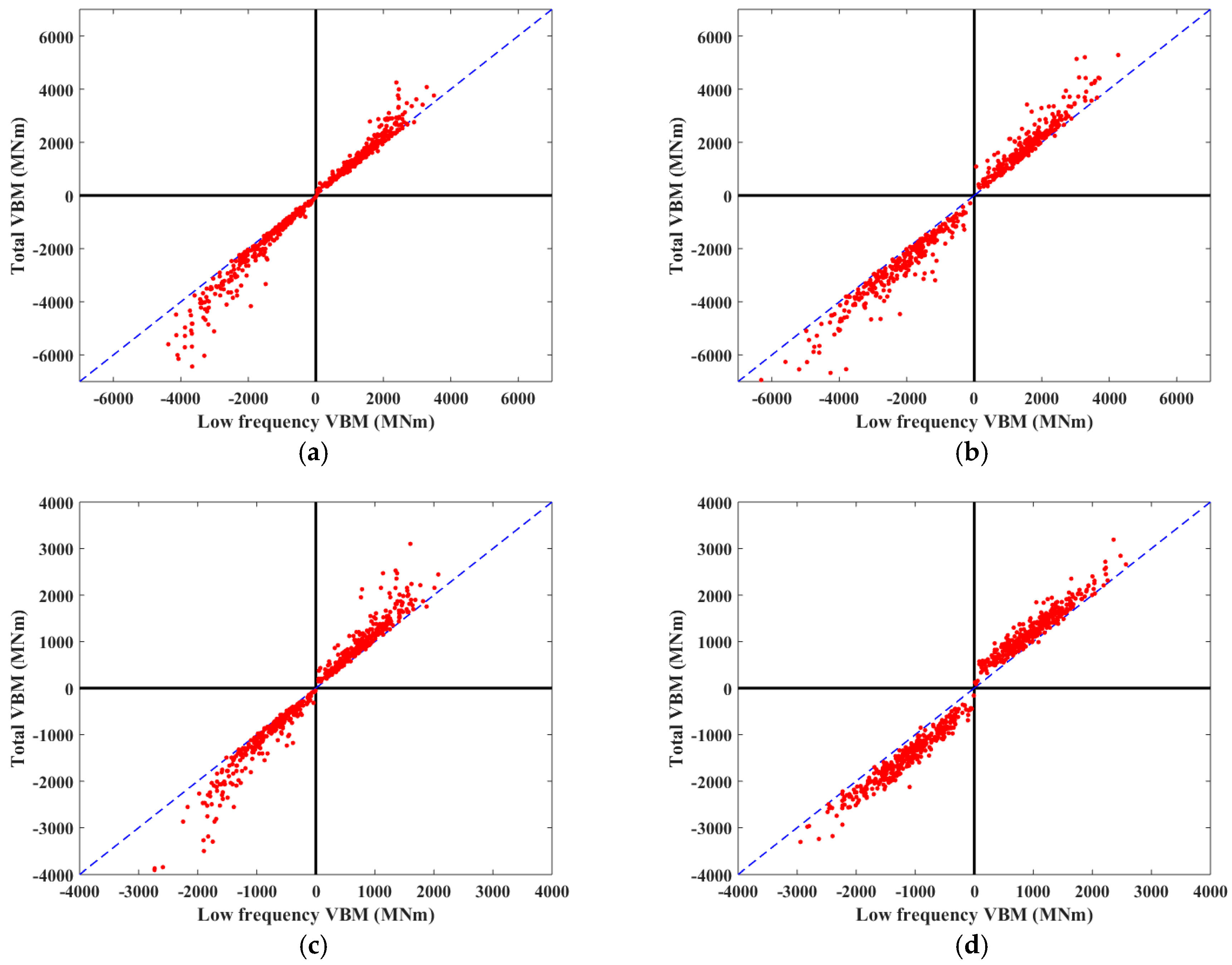
To further investigate the relationship between the low frequency M_BVs and the total M_BVs, the corresponding scatter diagrams are drawn in Figure 30, where the hogging and sagging M_BVs for both low frequency M_BVs (obtained by Fourier filtering mentioned above) and total M_BVs in each wave encountering period are counted and presented. The points in first and third quadrants denote hogging and sagging M_BVs, respectively. The diagonal that separates both the first and third quadrants into two equal parts denotes that the low frequency M_BVs are equal to the total M_BVs, meaning that the high frequency slamming M_BVs are zero. As illustrated in Figure 30, the high frequency slamming M_BVs have more effects on the sagging M_BVs than the hogging counterparts. The nonlinear behavior is more pronounced for experimental results than numerical results, especially for the higher speed condition, which can be explained by the fact that only weakly nonlinear effects are considered in the present hydroelasticity theory.

5. Conclusions

The present research proposes a 3D time domain nonlinear hydroelastic method to numerically estimate the vibrational responses of a large ship advancing in regular and irregular waves. A self-propelled segmented ship model was designed and tested in a towing tank to validate the numerical method presented in this study. The main findings from the presented experimental and numerical studies are as follows:

(1)

The presented time domain 3D nonlinear hydroelastic method is capable of predicting the hydroelastic vibrational responses of motions and vertical bending moments of large ships with pronounced bow flares sailing in both regular and irregular waves. The numerical results of motions of heave and pitch and M_BVs are satisfactorily validated by the results of self-propelled segmented model tests.

(2)

By comparing numerical and experimental results of heave and pitch responses in regular waves, evident oscillations in experimental peaks and troughs of motion responses can be detected due to the effect of velocity change and the uncertainty associated with the generation of experimental regular waves. Small asymmetric characteristics in peaks and troughs can be found in motion responses because of the nonlinearity associated with the hull geometry. Moreover, compared with the low frequency and high frequency components, the total M_BVs show significant asymmetric characteristics in peaks and troughs resulting from the contribution of ship hull geometry nonlinearity and the high frequency slamming components.

(3)

Either large wave amplitude or high ship velocity will increase the occurrence frequencies of slamming events in irregular wave conditions. Compared with ship velocity, the wave amplitude plays a more important role in the determination of M_BVs. The slamming phenomena have relatively small influence on heave and pitch motions, while they have significant effects on M_BVs. The high frequency M_BVs caused by slamming largely increase the total M_BVs on the basis of low frequency M_BVs, contributing greatly to the asymmetric characteristics of the total M_BVs in irregular wave conditions. Therefore, the slamming loads should be given more attention at ship design stage for structural design and evaluation.

(4)

For irregular wave conditions, the current research focuses on the statistical parameters of ship hydroelastic responses, since the experimental and numerical irregular waves are just compared statistically. The future study should compare the numerical and experimental irregular waves in fine details of their time series by monitoring the near-ship experimental irregular waves, and therefore, the experimental and numerical ship vibrational responses can be compared in fine details. In this way, some uncertainties associated with the randomly-generated irregular waves can be reduced, which currently results in the evident difference between experimental and numerical statistical parameters of ship responses. In addition, the evident difference between the numerical and experimental mean values of ship responses in irregular waves indicates that, before each run of the ship model, the water surface should be sufficiently calm to reduce the error associated with the choice of the balance position of the ship model.

References

- Bishop, R.E.D.; Price, W.G. The generalized antisymmetric fluid forces applied to a ship in a seaway. Int. Shipbuild. Prog. 1977, 24, 3–14. [Google Scholar] [CrossRef]
- Bishop, R.E.D.; Price, W.G. Hydroelasticity of Ships; Cambridge University Press: Cambridge, UK, 1979. [Google Scholar]
- Hermundstad, O.A.; Aarsns, J.V.; Moan, T. Linear hydroelastic analysis of high-speed catamarans and monohulls. J. Ship Res. 1999, 43, 48–63. [Google Scholar]
- Yamamoto, Y.; Fujino, M.; Fukasawa, T. Motion and longitudinal strength of a ship in head sea and the effects of non-linearities. Naval architecture and ocean engineering. J. Soc. Nav. Arch. Jpn. 1980, 18, 91–100. [Google Scholar]
- Hirdaris, S.E.; Temarel, P. Hydroelasticity of ships: Recent advances and future trends. J. Eng. Marit. Environ. 2009, 223, 305–330. [Google Scholar] [CrossRef]
- Wu, Y.S.; Cui, W.C. Advances in the three-dimensional hydroelasticity of ships. J. Eng. Marit. Environ. 2009, 223, 331–348. [Google Scholar] [CrossRef]
- Kim, J.H.; Kim, Y.; Yuck, R.H.; Lee, D.Y. Comparison of slamming and whipping loads by fully coupled hydroelastic analysis and experimental measurement. J. Fluids Struct. 2015, 52, 145–165. [Google Scholar] [CrossRef]
- Kim, J.H.; Kim, Y. Numerical analysis on springing and whipping using fully-coupled FSI models. Ocean Eng. 2014, 91, 28–50. [Google Scholar] [CrossRef]
- Fonseca, N.; Guedes Soares, C. Comparison of numerical and experimental results of nonlinear wave-induced vertical ship motions and loads. J. Mar. Sci. Technol. 2002, 6, 193–204. [Google Scholar] [CrossRef]
- Oberhagemann, J.; Shigunov, V.; El Moctar, O. Application of CFD in long-term extreme value analyses of wave loads. Ship Technol. Res. 2012, 59, 4–22. [Google Scholar] [CrossRef]
- Takami, T.; Matsui, S.; Oka, M.; Iijima, K. A numerical simulation method for predicting global and local hydroelastic response of a ship based on CFD and FEA coupling. Mar. Struct. 2018, 59, 368–386. [Google Scholar] [CrossRef]
- Zhu, S.; Moan, T. New insight into the wave-induced nonlinear vertical load effects of ultra-large container ships based on experiments. J. Mar. Sci. Technol. 2013, 18, 87–114. [Google Scholar] [CrossRef]
- Lavroff, J.; Davis, M.R.; Holloway, D.S.; Thomas, G. Wave slamming loads on wave-piercer catamarans operating at high-speed determined by hydro-elastic segmented model experiments. Mar. Struct. 2013, 33, 120–142. [Google Scholar] [CrossRef]
- Wang, X.L.; Gu, X.K.; Hu, J.J. Springing investigation of a ship based on model tests and 3D hydroelastic theory. J. Ship Mech. 2012, 16, 915–925. [Google Scholar]
- Grigoropoulos, G.J.; Katsaounis, G.M. Measuring Procedures for Seakeeping Tests of Large-Scaled Ship Models at Sea. In Proceedings of the 13th IMEKO TC4 Symposium on Measurements for Research and Industrial Applications, Athens, Greece, 29 September–1 October 2004; pp. 135–139. [Google Scholar]
- Jiao, J.L.; Sun, S.Z.; Li, J.D.; Adenya, C.A.; Ren, H.L.; Chen, C.H. A comprehensive study on the seakeeping performance of high speed hybrid ships by 2.5D theoretical calculation and different scaled model experiments. Ocean Eng. 2018, 160, 197–223. [Google Scholar] [CrossRef]
- Kim, Y.; Kim, B.-H.; Choi, B.-K.; Park, S.-G.; Malenica, S. Analysis on the full scale measurement data of 9400TEU container Carrier with hydroelastic response. Ocean Eng. 2016, 122, 293–310. [Google Scholar] [CrossRef]
- Jiao, J.L.; Ren, H.L.; Sun, S.Z.; Liu, N.; Li, H.; Adenya, C.A. A state-of-the-art large scale model testing technique for ship hydrodynamics at sea. Ocean Eng. 2016, 123, 174–190. [Google Scholar] [CrossRef]
- Kim, Y.; Kim, J.-H. Benchmark Study on Motions and Loads of a 6750-TEU Containership. Ocean Eng. 2016, 119, 262–273. [Google Scholar] [CrossRef]
- Clauss, G.F.; Klein, M. Experimental investigation on the vertical bending moment in extreme sea states for different hulls. Ocean Eng. 2016, 181–192. [Google Scholar] [CrossRef]
- Dai, Y.S.; Duan, W.Y. Potential Flow Theory of Ship Motions in Waves; National Defense Industry Press: Beijing, China, 2008. [Google Scholar]
- Hermans, A.J. Mechanics of Fluids and Transport Processes. In Water Waves and Ship Hydrodynamics: An Introduction; Springer: Berlin, Germany, 2011; pp. 1–169. [Google Scholar]
- Newman, J.N. The Approximation of Free-Surface Green Functions. In Wave Asymptotics; Cambridge University Press: Cambridge, UK, 1992. [Google Scholar]
- Li, H. 3-D Hydroelasticity Analysis Method for Wave Loads of Ships. Ph.D. Thesis, Harbin Engineering University, Harbin, China, 2009. [Google Scholar]
- Chen, Z.Y.; Jiao, J.L.; Li, H. Time-domain numerical and segmented ship model experimental analyses of hydroelastic responses of a large container ship in oblique regular waves. Appl. Ocean Res. 2017, 67, 78–93. [Google Scholar] [CrossRef]
- Wehausen, J.V. The motion of Floating bodies. Annu. Rev. Fluid Mech. 1971, 3, 237–268. [Google Scholar] [CrossRef]
- Salvesen, N.; Tuck, E.O.; Faltinsen, O. Ship Motions and Sea Loads; SNAME: Alexandria, VA, USA, 1970. [Google Scholar]
- Von Karman, T. The Impact on Seaplane Floats during Landing; NACA TN321; National Advisory Committee for Aeronautics: Washington, DC, USA, 1929. [Google Scholar]
- Wu, Y.S. Hydroelasticity of Floating Bodies. Ph.D. Thesis, Brunel University, London, UK, 1984. [Google Scholar]
- Thomson, W.T. Theory of Vibration with Applications, 2nd ed.; Prentice-Hall: Upper Saddle River, NJ, USA, 1981. [Google Scholar]
- Rosinger, H.E.; Ritchie, I.G. On Timoshenko’s correction for shear in vibrating isotropic beams. J. Phys. D Appl. Phys. 1977, 10, 1461–1466. [Google Scholar] [CrossRef]
- Burden, R.L.; Faires, D.J.; Burden, A.M. Numerical Analysis; Brooks Cole: Boston, MA, USA, 2015. [Google Scholar]
- Singh, S.P.; Sen, D. A comparative study on 3D wave load and pressure computations for different level of modelling of nonlinearities. Mar. Struct. 2007, 20, 1–24. [Google Scholar] [CrossRef]
- Seakeeping committee of the 27th ITTC. ITTC-Recommended Procedures and guidelines-Seakeeping experiments. 2014; 1–22.
- Adolfo, M.; Geert, K. Design of a ship model for hydro-elastic experiments in waves. Int. J. Nav. Archit. Ocean Eng. 2014, 6, 1130–1147. [Google Scholar]
- Riccardo, M.; Daniele, D. Analysis of the global bending modes of a floating structure using the proper orthogonal decomposition. J. Fluids Struct. 2012, 28, 115–134. [Google Scholar]
- Li, H.; Wang, D.; Liu, N.; Zhou, X.Q.; Chen Ong, M. Influence of Linear Springing on the Fatigue Damage of Ultra Large Ore Carriers. Appl. Sci. 2018, 8, 763. [Google Scholar] [CrossRef]
Figure 1.
Mathematical description of ship-fluid interaction.
Figure 2.
Overview of the model setup.
Figure 3.
General arrangement of elastic backbones.
Figure 4.
The ship model towing tank. (a) Wave tank at work; (b) Wave generator
Figure 5.
Mesh information. (a) Panels of the whole hull surface; (b) Panels of the wet surface for [FR] and [FD].
Figure 6.
Uneven cross sections for calculation of slamming loads.
Figure 7.
Acquisition of instantaneous wetted surface during computation.
Figure 8.
Added mass coefficients. (a) A33; (b) A55
Figure 9.
Damping coefficients. (a) B33; (b) B55
Figure 10.
Retardation functions. (a) K33; (b) K55
Figure 11.
First three elastic modes.
Figure 12.
Effects of orders of elastic modes on total MBVs amidships (ship velocity: 18 kn, wave height: 9 m, wave period: 13.28 s).
Figure 13.
Experimentally measured time series of regular wave condition 2.
Figure 14.
Motion response in regular wave condition 1. (a) Heave (m); (b) Pitch (deg)
Figure 15.
Motion response in regular wave condition 2. (a) Heave (m); (b) Pitch (deg)
Figure 16.
Motion responses at different wave heights (V = 18 kn, λ/L = 1.0). (a) Heave responses; (b) Pitch responses.
Figure 17.
Total MBV in regular waves. (a) Regular wave condition 1; (b) Regular wave condition 2
Figure 18.
Low frequency MBV in regular waves. (a) Regular wave condition 1; (b) Regular wave condition 2.
Figure 19.
High frequency MBV in regular waves. (a) Regular wave condition 1; (b) Regular wave condition 2.
Figure 20.
MBV responses at different wave heights (V = 18 kn, λ/L = 1.0). (a) Total MBV; (b) Low frequency MB; (c) High frequency MBV.
Figure 21.
Experimentally measured time series of irregular wave condition 2.
Figure 22.
Comparison of wave spectra. (a) Irregular wave condition 1; (b) Irregular wave condition 2.
Figure 23.
Heave responses in irregular wave condition 1. (a) Experimental result; (b) Numerical result
Figure 24.
Pitch responses in irregular wave condition 1. (a) Experimental result; (b) Numerical result
Figure 25.
Heave responses in irregular wave condition 2. (a) Experimental result; (b) Numerical result
Figure 26.
Pitch responses in irregular wave condition 2. (a) Experimental result; (b) Numerical result.
Figure 27.
Time history of MBVs amidships in irregular wave condition 1. (a) Experimental result of total MBV; (b) Numerical result of total MBV; (c) Experimental result of low frequency MBV; (d) Numerical result of low frequency MBV; (e) Experimental result of high frequency MBV; (f) Numerical result of high frequency MBV.
Figure 28.
Time history of MBV amidships in irregular wave condition 2. (a) Experimental result of total MBV; (b) Numerical result of total MBV; (c) Experimental result of low frequency MBV; (d) Numerical result of low frequency MBV; (e) Experimental result of high frequency MBV; (f) Numerical result of high frequency MBV.
Figure 29.
Probability of exceedance of total MBV responses in irregular waves. (a) Irregular wave condition 1; (b) Irregular wave condition 2.
Figure 30.
Relationship between low frequency MBVs and total MBVs. (a) Experimental result for irregular condition 1; (b) Numerical result for irregular condition 1; (c) Experimental result for irregular condition 2; (d) Numerical result for irregular condition 2.