Propagation of Optical Coherence Vortex Lattices in Turbulent Atmosphere

Abstract

Propagation properties in the turbulence atmosphere of the optical coherence vortex lattices (OCVLs) are explored by the recently developed convolution approach. The evolution of spectral density distribution, the normalized $M^2$-factor, and the beam wander of the OCVLs propagating through the atmospheric turbulence with Tatarskii spectrum are illustrated numerically. Our results show that the OCVLs display interesting propagation properties, e.g., the initial Gaussian beam distribution will evolve into hollow array distribution on propagation and finally becomes a Gaussian beam spot again in the far field in turbulent atmosphere. Furthermore, the OCVLs with large topological charge, large beam array order, large relative distance, and small coherence length are less affected by the negative effects of turbulence. Our results are expected to be used in the complex system optical communications.

1. Introduction

Optical lattices can be viewed as a typical kind of beam arrays, which display sufficiently small beam spots. Recently, a novel class of optical lattices, which are named optical coherence lattices (OCLs), were introduced by Ma and Ponomarenko [1]. The OCLs were described with the help of the complex Gaussian representation and the time-domain OCLs were generated through superposition of Gaussian pulses [2]. The property of periodic reciprocity of the OCLs on propagation through the free-space was found [3]. Periodic reciprocity means the periodic degree of coherence at the source plane transfers the periodicity to the transverse intensity distribution after a long propagation distance. Recently, both scalar and vector OCLs were generated in experiment [4,5]. Furthermore, other kinds of optical lattices were also proposed [6,7,8]. The optical lattices were found to be useful in various applications, e.g., image transmission and encryption [4], trapping and cooling atoms [9], photonic crystals engineering [10], lattice light-sheet microscopy [11], and ultracold trapping of quantum gas [12].

On the other hand, partially coherent beams have been studied extensively over the last few decades due to their novel physical properties and widely uses in various fields, such as free-space optical communications, optical imaging, particle trapping, particle scattering, and remote detection. The statistical properties, e.g., degree of coherence [13], beam spreading [14,15], propagation factor [16,17,18], Rayleigh range [19], and scintillation index [20,21,22] of different kinds of partially coherent beams in free space and in various turbulent atmosphere have been studied in detail. The propagation properties of the OCLs (i.e., a typical kind of partially coherent beams with periodical degree of coherence) in atmospheric turbulence were explored [23], and the results showed that the OCLs have an advantage of mitigating scintillation index in atmospheric turbulence on propagation.

A vortex beam with twisted wavefront carries an orbital angular momentum and has various applications ranging from optical tweezers to optical communications [24,25,26,27,28]. The topological charge (which defines how the wavefront of the vortex beam twists) on propagation in atmospheric turbulence is robust [29]. In 1998, Gori et al. introduced a class of partially coherent beams with helical wavefront, which were named partially coherent vortex beams (PCVB) [30]. Subsequently, efforts have been made to the PCVBs [31,32,33,34,35,36,37,38,39,40,41,42,43,44]. A review on propagation, generation, and measurement of PCVBs was given [41], and self-healing properties of a PCVB was found [42]. More recently, PCVB with a fractional topological charge [43] and partially coherent vortex beam with periodical degree of coherence (i.e., optical coherence vortex lattices) [44] were introduced, respectively. In this paper, we investigate the statistical properties (i.e., spectral density distribution, normalized M²-factor, and beam wander) of optical coherence vortex lattices (OCVLs) in turbulent atmosphere by using the recently developed convolution approach. We find that the initial Gaussian beam distribution of the OCVLs evolves into hollow array distribution on propagation and finally becames a Gaussian beam spot again in the far field in turbulent atmosphere. The OCVLs with prescribed beam parameters are less affected by the turbulence, which will be useful for free-space optical communications.

2. Formulation of the Propagation of OCLVs in Turbulent Atmosphere

The second-order properties of a partially coherent beam in frequency domain can be studied by the cross-spectral density (CSD) function. To construct a bona fide field, the CSD function at source can be expanded as follows [45]:

$$W\left({\mathbf{r}}_1,{\mathbf{r}}_2;0\right)={\displaystyle \int p\left(\mathbf{v}\right)}{H}^{\ast }\left({\mathbf{r}}_1,\mathbf{v}\right)H\left({\mathbf{r}}_2,\mathbf{v}\right)d^2\mathbf{v},$$

(1)

where ${\mathbf{r}}_1=(x_1,y_1)$ and ${\mathbf{r}}_2=(x_2,y_2)$ are the two arbitrary transverse position vectors at source plane, $p\left(\mathbf{v}\right)$ is a scalar nonnegative function, $H\left(\mathbf{r},\mathbf{v}\right)$ denotes an arbitrary suitable kernel function.

To generate OCVLs, we define $p\left(\mathbf{v}\right)$ and $H\left(\mathbf{r},\mathbf{v}\right)$ as follows:

$$p\left(\mathbf{v}\right)=\frac{1}{M}{\displaystyle \sum _{m=-\left(M-1\right)/2}^{\left(M-1\right)/2}\exp \left[-\frac{{\left|\mathbf{v}-{\mathbf{v}}_{0m}\right|}^2}{2w_0^2}\right]},$$

(2)

$$H\left(\mathbf{r},\mathbf{v}\right)=-\frac{i}{\lambda f}\tau \left(\mathbf{r}\right)\exp \left[\frac{i\pi }{\lambda f}\left({\mathbf{v}}^2-2\mathbf{r}\cdot \mathbf{v}\right)\right].$$

(3)

where $p\left(\mathbf{v}\right)$ is superposed by the M space-shifted Gaussian functions, $w_0$ and ${\mathbf{v}}_{0m}=\left(md,md\right)$ denote the circular aperture radius and the position vector of the lattices, respectively, and $d$ denotes the distance between adjacent spots. $H\left(\mathbf{r},\mathbf{v}\right)$ represents in the experiment the response function of an optical Fourier transform system consisting of a free-space distance of f, a thin lens with focal distance f, and an optical filter with transmission function $\tau \left(\mathbf{r}\right)$ [44]. Here we set $\tau \left(\mathbf{r}\right)$ in the cylindrical coordinates as follows:

$$\tau \left(r,\theta \right)={\left(\frac{\sqrt{2}r}{{\omega }_0}\right)}^l\exp \left(-\frac{r^2}{{\omega }_0^2}\right)\exp \left(-il\theta \right),$$

(4)

where $l$ and ${\omega }_0$ are the topological charge and beam width, respectively, $\left(r, \theta \right)$ are cylindrical polar coordinates.

By substituting Equations (2)–(4) into Equation (1), the CSD of the OCVLs at source plane is obtained as follows:

$$\begin{array}{ll}{W}_0(r_1,{\theta }_1,r_2,{\theta }_2)& =\frac{2w_0^2\pi }{M{\lambda }^2{f}^2}{\displaystyle \sum _{m=-\left(M-1\right)/2}^{\left(M-1\right)/2}{\left(\frac{2r_1{r}_2}{{\omega }_0^2}\right)}^l\exp \left(-\frac{r_1^2+r_2^2}{{\omega }_0^2}\right)\exp \left[il({\theta }_2-{\theta }_1)\right]}\\ & \times \exp \left[-\frac{r_1^2+r_2^2-2r_1{r}_2\cos \left({\theta }_2-{\theta }_1\right)}{2{\delta }_0^2}\right]\\ & \times \exp \left\{-b\left[\left(r_2\cos {\theta }_2-r_1\cos {\theta }_1+r_2\sin {\theta }_2-r_1\sin {\theta }_1\right)\right]\right\},\end{array}$$

(5)

where ${\delta }_0=f/\left(w_{0}k\right)$ is the beam initial coherence width. For the convenience of calculation, we set $a=1/2{\delta }_0^2=2w_0^2{\pi }^2/({\lambda }^2{f}^2),b=2i\pi md/\left(\lambda f\right)$.

The spectral density of a propagating partially coherent beam in turbulent atmosphere can be obtained by using the convolution approach as follows [46]:

$$S\left(\mathsf{\rho },z\right)=S_f\left(-\mathsf{\rho }/z\right)\otimes p_1\left(-\mathsf{\rho }/z\right)\otimes p_2\left(-\mathsf{\rho }/z\right),$$

(6)

where $\mathsf{\rho }$ is the position vector in the receiver plane with the propagation distance being $z$. $S_f\left(-\mathsf{\rho }/z\right)$ is the spectral density of the incoherent portion on propagation in free space, $p_1\left(-\mathsf{\rho }/z\right)$ is the Fourier transform of the degree of coherence of the beam at source plane, $p_2\left(-\mathsf{\rho }/z\right)$ is the Fourier transform of second-order random phase correlation function, and $\otimes$ is the symbol of convolution.

According to the Huygens-Fresnel integral, $S_f\left(-\mathsf{\rho }/z\right)$ is obtained by:

$$S_f\left(-\mathsf{\rho }/z\right)={\left|\tilde{A}\left(\mathsf{\rho }/z\right)\right|}^2/{\lambda }^2{z}^2,$$

(7)

where $A\left(\mathbf{r}\right)=\tau \left(\mathbf{r}\right)\exp \left(ik{\mathbf{r}}^2/2z\right)$ and the hat tilde denotes the two-dimensional Fourier transform, and [47]:

$$p_2\left({\mathbf{v}}^{\prime }\right)=\frac{3}{2{\pi }^{3}Tz}\exp \left(-\frac{3{{\mathbf{v}}^{\prime }}^2}{2{\pi }^{2}Tz}\right),$$

(8)

with:

$$T={\displaystyle {\int }_{-\infty }^{\infty }{\kappa }^3{\mathsf{\Phi }}_n\left(\kappa \right)}d\kappa .$$

(9)

Here ${\mathsf{\Phi }}_n\left(\kappa \right)$ is the power spectrum density of the atmospheric turbulence refractive index fluctuations, $\kappa$ denotes the frequency in the space. Here we adopted the Tatarskii spectrum for the power spectrum density ${\mathsf{\Phi }}_n\left(\kappa \right)$, which is written as [48]:

$${\mathsf{\Phi }}_n\left(\kappa \right)=0.033C_n^2{\kappa }^{-11/3}\exp \left(-\frac{{\kappa }^2}{{\kappa }_m^2}\right).$$

(10)

Here $C_n^2$ denotes the structure parameter of the atmospheric turbulence and ${\kappa }_m=5.92/l_0$ with $l_0$ being the turbulence inner scale. In this paper, we set $l_0=0.01\mathrm{m}$. Taking Equation (10) into Equation (9), we obtain:

$$T=0.771C_n^2.$$

(11)

Taking Equations (2), (4), (7), and (8) into Equation (6), and using the fast Fourier transform (FFT) algorithm, one can numerically analyze the spectral density of the OCVLs propagating in turbulent atmosphere by using MATLAB (The MathWorks, Natick, MA, USA).

For further investigating the propagation properties of the OCVLs, we also study the $M^2$-factor and beam wander [49,50,51]. The beam’s second-order moments in turbulent atmosphere in the receiver plane are obtained as follows [51]:

$$\langle r^2\rangle ={\langle r^2\rangle }_0+2{\langle \mathbf{r}\cdot \mathsf{\theta }\rangle }_{0}z+{\langle {\theta }^2\rangle }_0{z}^2+\frac{4}{3}{\pi }^{2}T{z}^3,$$

(12)

$$\langle {\theta }^2\rangle ={\langle {\theta }^2\rangle }_0+4{\pi }^{2}Tz,$$

(13)

$$\langle \mathbf{r}\cdot \mathsf{\theta }\rangle ={\langle \mathbf{r}\cdot \mathsf{\theta }\rangle }_0+{\langle {\theta }^2\rangle }_{0}z+2{\pi }^{2}T{z}^2,$$

(14)

By the partial derivative method, the second-order moments of the partially coherent beams at source plane can be obtained by [52]:

$${\langle r^2\rangle }_0=\frac{1}{I}{\displaystyle {\int }_0^{2\pi }{\displaystyle {\int }_0^{\infty }{r}^3}{W}_0(r,\theta ,r,\theta )drd\theta },$$

(15)

$${\langle {\theta }^2\rangle }_0=\frac{1}{k^{2}I}{\displaystyle {\int }_0^{2\pi }{\displaystyle {\int }_0^{\infty }\left\{\frac{{\partial }^2{W}_0(r_1,{\theta }_1,r_2,{\theta }_2)}{\partial r_1\partial r_2}|{}_{\begin{array}{l}{r}_1=r_2=r\\ {\theta }_1={\theta }_2=\theta \end{array}}+\frac{1}{r^2}\frac{{\partial }^2{W}_0(r_1,{\theta }_1,r_2,{\theta }_2)}{\partial {\theta }_1\partial {\theta }_2}|{}_{\begin{array}{l}{r}_1=r_2=r\\ {\theta }_1={\theta }_2=\theta \end{array}}\right\}}rdrd\theta },$$

(16)

$${\langle r\theta \rangle }_0=\frac{1}{ikI}{\displaystyle {\int }_0^{2\pi }{\displaystyle {\int }_0^{\infty }\left\{r_1\frac{\partial W_0(r_1,{\theta }_1,r_2,{\theta }_2)}{\partial r_1}-r_2\frac{\partial W_0(r_1,{\theta }_1,r_2,{\theta }_2)}{\partial r_2}\right\}|\begin{array}{l}\\ {}_{\begin{array}{l}{r}_1=r_2=r\\ {\theta }_1={\theta }_2=\theta \end{array}}\end{array}}rdrd\theta },$$

(17)

where $k = 2\pi /\lambda$ denotes the wavenumber, and:

$$I={\displaystyle {\int }_0^{2\pi }{\displaystyle {\int }_0^{\infty }W(r,\theta ,r,\theta ;0)}rdrd\theta },$$

(18)

is the total energy for the beam.

By substituting Equations (5), (15)–(17) into Equations (12)–(14), we obtained:

$$\langle r^2\rangle =\frac{{\omega }_0^2\left(l+1\right)}{2}+\frac{{\lambda }^2{z}^2}{4{\pi }^2}\left[4a+\frac{2\left(l+1\right)}{{\omega }_0^2}-\frac{2}{M}{\displaystyle \sum _{m=-\left(M-1\right)/2}^{\left(M-1\right)/2}{b}^2}\right]+\frac{4}{3}{\pi }^{2}T{z}^3,$$

(19)

$$\langle {\theta }^2\rangle =\frac{{\lambda }^2}{4{\pi }^2}\left[4a+\frac{2\left(l+1\right)}{{\omega }_0^2}-\frac{2}{M}{\displaystyle \sum _{m=-\left(M-1\right)/2}^{\left(M-1\right)/2}{b}^2}\right]+4{\pi }^{2}Tz,$$

(20)

$$\langle r\theta \rangle =\frac{{\lambda }^{2}z}{4{\pi }^2}\left[4a+\frac{2\left(l+1\right)}{{\omega }_0^2}-\frac{2}{M}{\displaystyle \sum _{m=-\left(M-1\right)/2}^{\left(M-1\right)/2}{b}^2}\right]+2{\pi }^{2}T{z}^2.$$

(21)

The $M^2$-factor is an important parameter to measure the laser quality and is defined as [51,52,53]:

$$M^2(z)=\frac{2\pi }{\lambda }{\left(\langle r^2\rangle \langle {\theta }^2\rangle -{\langle r\theta \rangle }^2\right)}^{1/2}.$$

(22)

The $M^2$-factor of OCVLs can be obtained by substituting Equations (19)–(21) into Equation (22). Our results agree well with the Ref. [40] when $M=1$ and $l=0$.

According to Ref. [51,52,53], we obtain the following expressions for the effective beam size:

$$W_{LT}=\sqrt{\frac{{\omega }_0^2\left(l+1\right)}{2}+\frac{{\lambda }^2{z}^2}{4{\pi }^2}\left[4a+\frac{2\left(l+1\right)}{{\omega }_0^2}-\frac{2}{M}{\displaystyle \sum _{m=-\left(M-1\right)/2}^{\left(M-1\right)/2}{b}^2}\right]+\frac{4}{3}{\pi }^{2}T{z}^3},$$

(23)

and in free space

$$W_{FS}=\sqrt{\frac{{\omega }_0^2\left(l+1\right)}{2}+\frac{{\lambda }^2{L}^2}{4{\pi }^2}\left[4a+\frac{2\left(l+1\right)}{{\omega }_0^2}-\frac{2}{M}{\displaystyle \sum _{m=-\left(M-1\right)/2}^{\left(M-1\right)/2}{b}^2}\right]}.$$

(24)

Beam wander is characterized by ${\langle r_c^2\rangle }^{1/2}$ of the variance of off-axis displacement of the instantaneous beam center. Beam wander is defined as follows [54]:

$$\langle r_c^2\rangle =\frac{16{\pi }^3}{{\lambda }^2}{W}_{FS}^2{\displaystyle {\int }_0^L{\displaystyle {\int }_0^{\infty }\kappa {\mathsf{\Phi }}_n\left(\kappa \right)}}\exp \left(-{\kappa }^2{W}_{LT}^2\right)\left\{1-\exp \left[\frac{-2L^2{\kappa }^2\left(1-z/L\right)}{k^2{W}_{FS}^2}\right]\right\}d\kappa dz,$$

(25)

taking Equation (10) into Equation (25), Equation (25) is simplified as:

$$\langle r_c^2\rangle =\frac{0.132}{\lambda }{\pi }^3{W}_{FS}^2\mathsf{\Gamma }\left(-5/6\right){\displaystyle {\int }_0^L\left\{{\left(2.85\times {10}^{-6}+W_{LT}^2\right)}^{5/6}-{\left[\frac{2L^2{\left(1-z/L\right)}^2}{k^2{W}_{FS}^2}+2.85\times {10}^{-6}+W_{LT}^2\right]}^{5/6}\right\}}dz,$$

(26)

the evolution properties of the beam wander in turbulent atmosphere of OCVLs can be calculated numerically by taking Equations (23) and (24) into Equation (26).

3. Numerical Results

3.1. Spectral Density Distribution

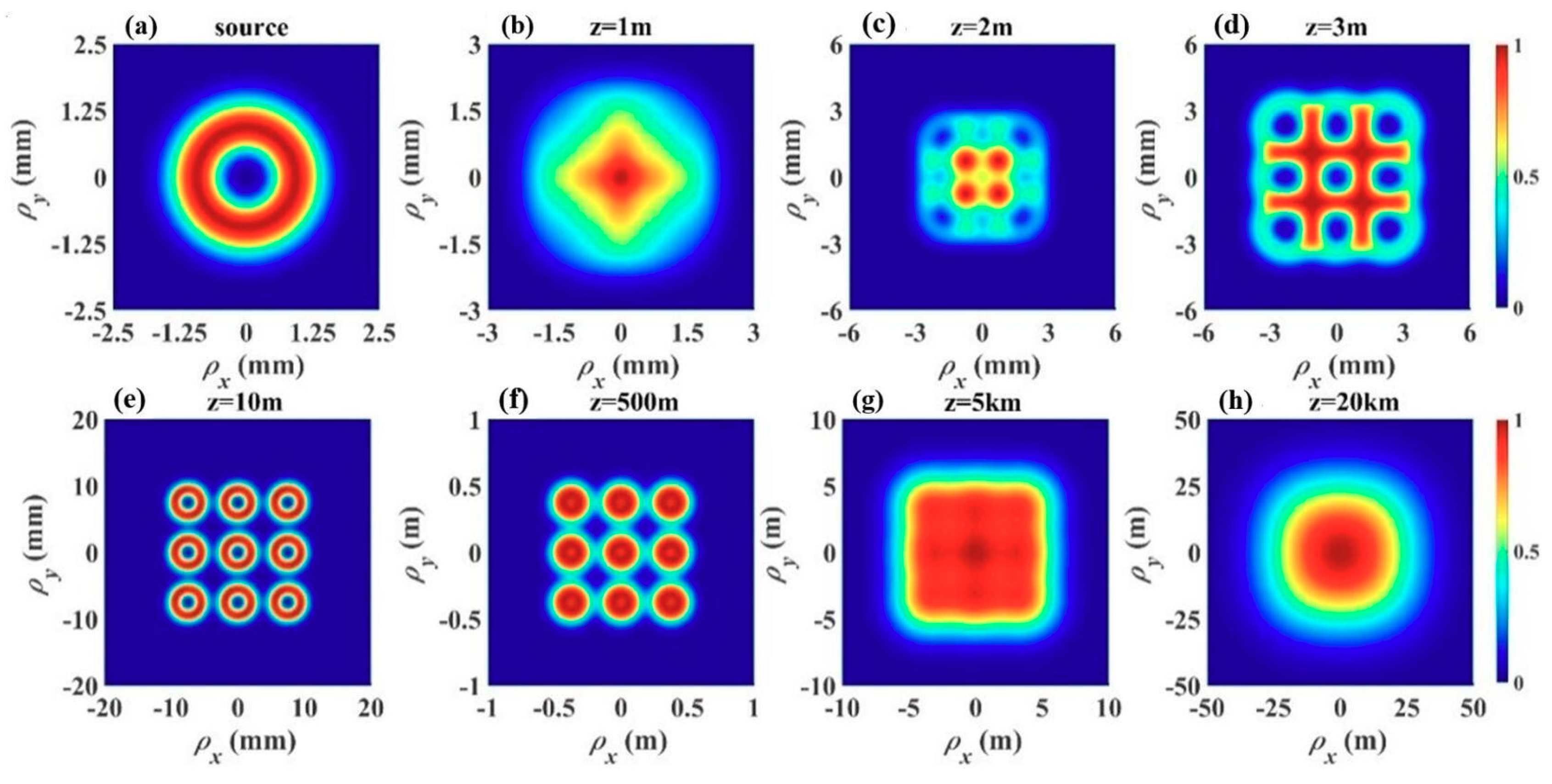
Figure 1 displays the spectral density distribution of the OCVLs in turbulent atmosphere at various propagation distances with $\lambda =532.8\mathrm{nm},M=3,l=2, {\omega }_0=1\mathrm{mm}, {\delta }_{0 }=3.4\mathrm{mm}, C_n^2={10}^{-13}{\mathrm{m}}^{-2/3}, \mathrm{and} d =0.3\mathrm{mm}.$ From Figure 1a, one finds that the spectral density distribution of the OCVLs at source is a single beam spot with doughnut beam profile. The single beam spot gradually evolves into $3\times 3$ hollow beam arrays (see Figure 1e) with the increase of the propagation distance$z$, which is similar to its evolution properties in free-space [44]. However, when we further increase the propagation distance, the effect of turbulence on beam properties accumulates gradually. The hollow beam arrays disappear gradually and finally become a Gaussian beam profile in the far field (see Figure 1h).

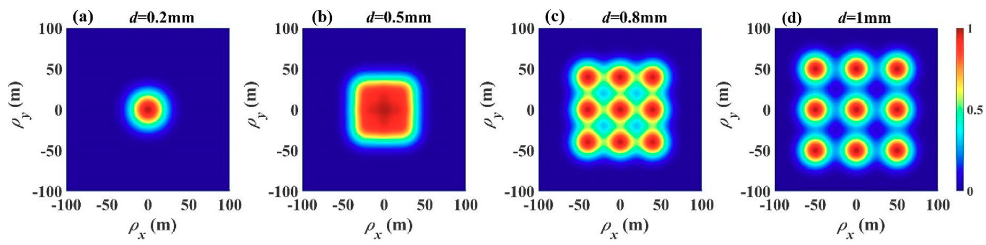
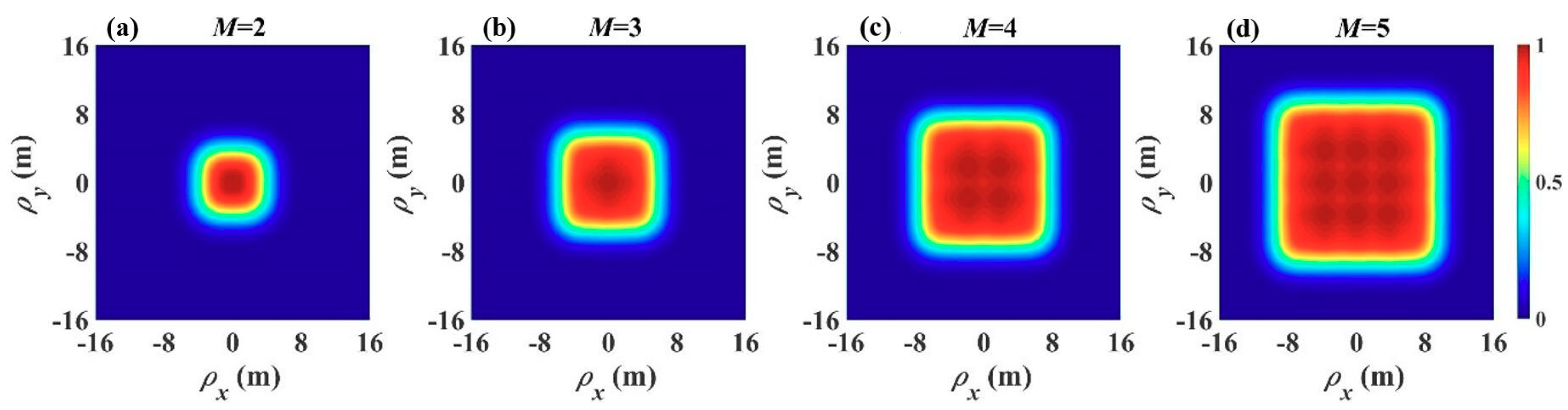
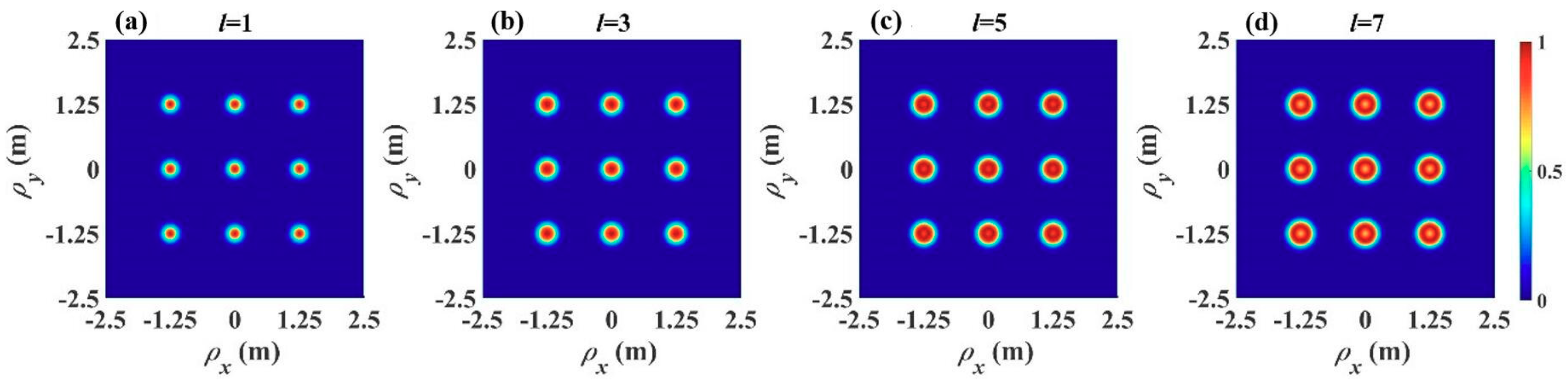
Figure 2 displays the spectral density distribution of the OCVLs in turbulent atmosphere at z = 5 km for several values of the relative distance $\mathrm{with}\lambda =532.8\mathrm{nm},M=3,l=2, {\omega }_0=1\mathrm{mm},{\delta }_0=3.4\mathrm{mm},\mathrm{and}{C}_n^2={10}^{-13}{\mathrm{m}}^{-2/3}$. From Figure 2, one sees that the beam distribution of the OCVLs evolves into Gaussian distribution rapidly when the relative distance $d$ is small (see Figure 2a). On the contrary, the beam array profile persists for longer distances when the relative distance $d$ increases (see Figure 2d). Figure 3 displays the spectral density of the OCVLs in turbulent atmosphere at $z=5\mathrm{km}$for several values of the array index $M$ with $\lambda =532.8\mathrm{nm},l=2, {\delta }_0=0.45\mathrm{mm}, {\omega }_0=1\mathrm{mm}, C_{n }^2={10}^{-13}{\mathrm{m}}^{-2/3},\mathrm{and}d=0.3\mathrm{mm}.$ From Figure 3, the beam spot size of the OCVLs increases as the array order $M$ increases, which indicates the OCVLs spread more rapidly as the array order M increases. Figure 4 displays the spectral density distribution of the OCVLs in turbulent atmosphere at $z=500\mathrm{m}$for several values of $l$ with $\lambda =532.8\mathrm{nm},M=3, {\delta }_0=0.7\mathrm{mm}, {\omega }_0=1\mathrm{mm}, C_{n }^2={10}^{-13} {\mathrm{m}}^{-2/3},\mathrm{and}d=1\mathrm{mm}$ (see Figure 4a). One finds that the beam arrays keep hollow profiles for longer propagation distances as the topological charge l increases, which means the OCVLs with large topological charges are less affected by turbulence.

3.2. $M^2$-Factor

In this subsection, we explore the evolution of the normalized $M^2$-factor of the OCVLs in turbulent atmosphere.

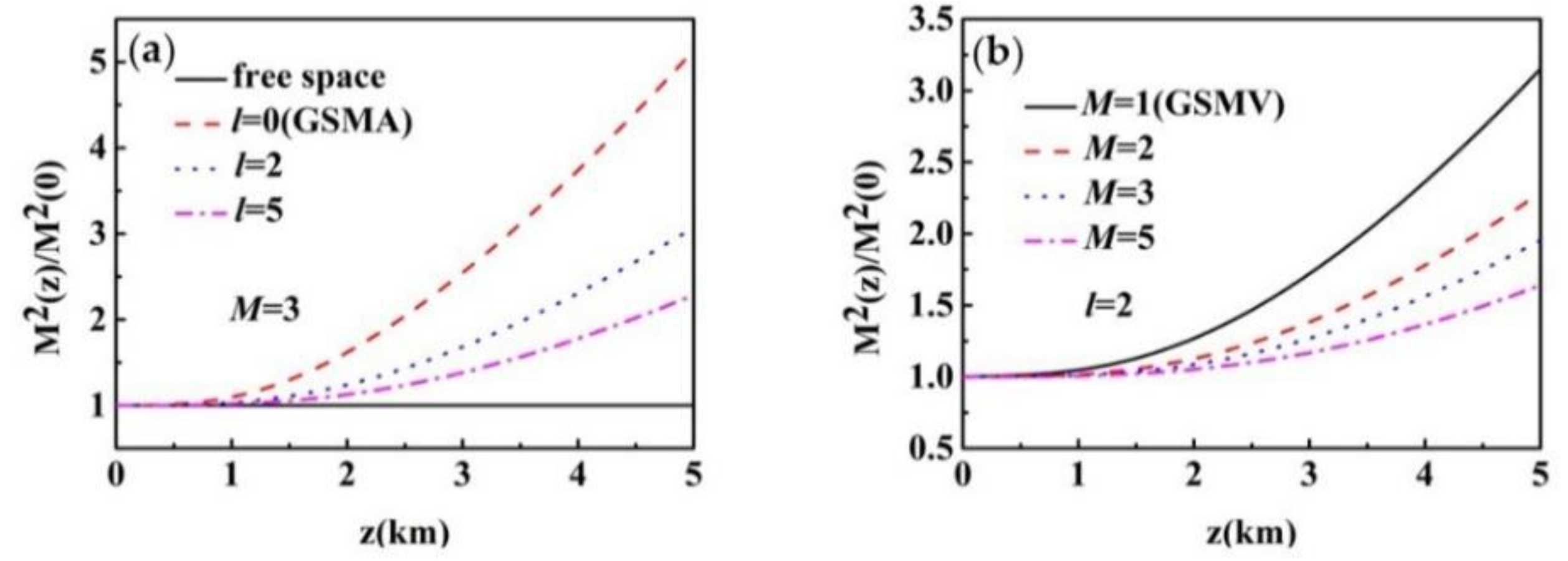
Figure 5 displays the normalized $M^2$-factor of the OCVLs in turbulent atmosphere for several different topological charge $l$ and beam array order $M$ with $\lambda =532.8\mathrm{nm}, C_n^2={10}^{-15} {\mathrm{m}}^{-2/3},d=1\mathrm{mm}, {\delta }_0=5\mathrm{mm},and{\omega }_0=1\mathrm{cm}.$ Figure 5a shows that as the normalized $M^2$-factor of the OCVLs remains invariant on propagation in free space ($C_n^2=0$), this property represents the best beam quality. However, for the turbulent atmosphere, the normalized $M^2$-factor of the OCVLs increases on propagation, and its value is smaller than that of the Gaussian Schell-model (GSM) array (l = 0) when the propagation distance is fixed. Furthermore, the normalized $M^2$-factor increases with the decrease of the topological charge $l$. From Figure 5b, one can see that the normalized $M^2$-factor of the OCVLs (M > 1) is smaller than that of the GSM vortex beam (M = 1), and the normalized $M^2$-factor increases as M decreases. Figure 5 indicates that the OCVLs will be less affected by the negative effects of the turbulence for larger topological charge and larger beam array order from the view point of the normalized $M^2$-factor.

3.3. Beam Wander

In this subsection, we explore the beam wander of the OCVLs in turbulent atmosphere for several different initial beam parameters.

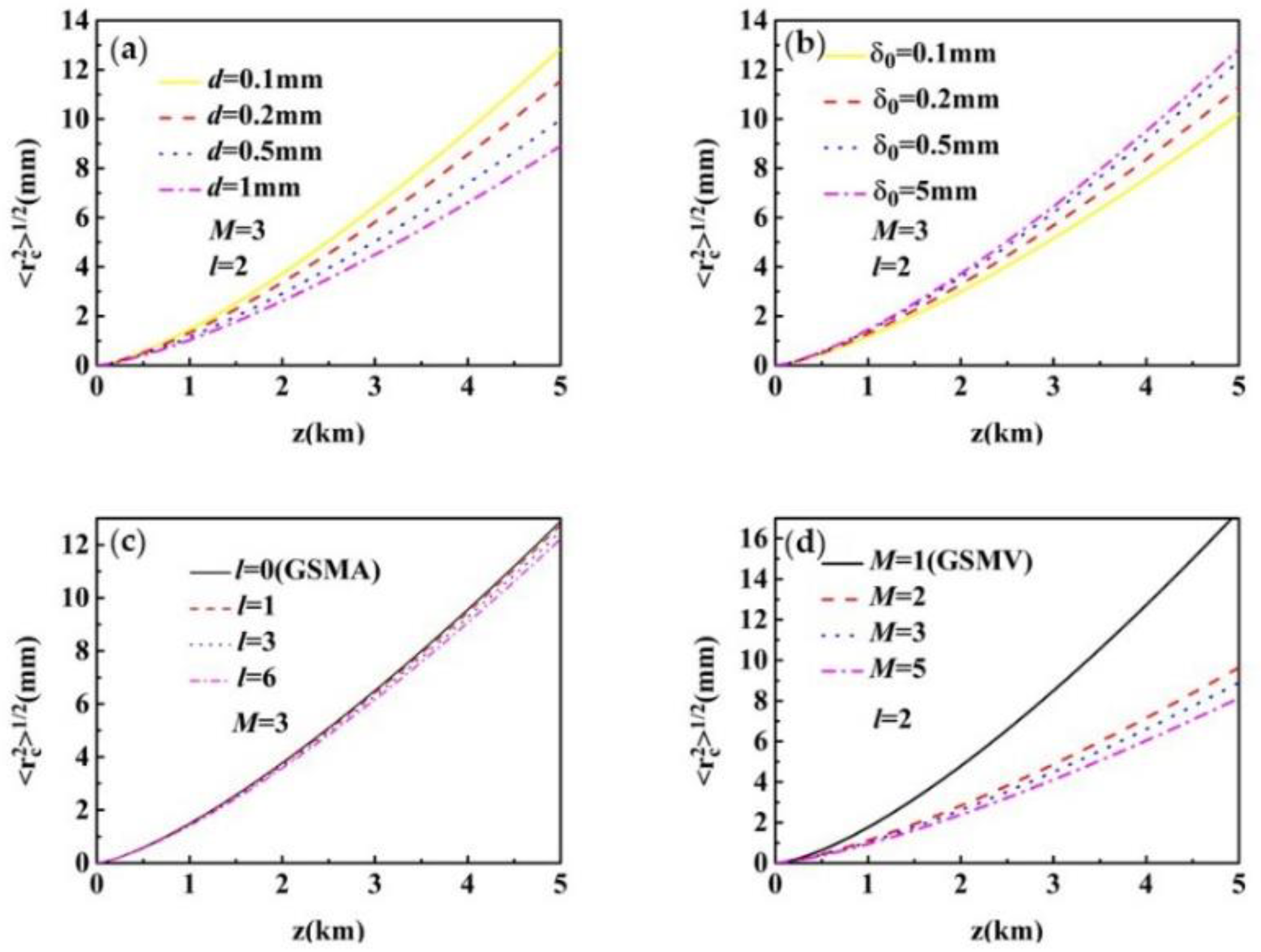
Figure 6 shows the beam wander of the OCVLs in turbulent atmosphere for various ${\delta }_0$, relative distance $d$, topological charges $l$, and beam array order $M$ with $\lambda =532.8\mathrm{nm},C_n^2={10}^{-15}{\mathrm{m}}^{-2/3},and{\omega }_0=1\mathrm{cm}.$From Figure 6, it is found that the beam wander of the OCVLs in turbulent atmosphere increases as the coherence width ${\delta }_0$ increases, or as the relative distance $d$, topological charge $l,$ and beam array order $M$ decrease, which means that the OCVLs are less affected by turbulence for large topological charge, large beam array order, large relative distance, and small coherence length from the view point of the beam wander.

4. Conclusions

We have formulated the propagation of the OCVLs in turbulent atmosphere by using the convolution approach, and we have explored propagation dynamics, such as the spectral density, the normalized $M^2$-factor, and the beam wander of the OCVLs in turbulent atmosphere. We have found that the beam distribution of the OCVLs changes from a single doughnut beam distribution to hollow array distribution on propagation, and finally becomes the Gaussian distribution in the far field. We also have found that the OCVLs with large topological charge, large beam array order, large relative distance, and small coherence length can mitigate the influence of atmospheric turbulence. Our findings are useful for free-space optical communications and information transfer.

References

- Ma, L.; Ponomarenko, S.A. Optical coherence gratings and lattices. Opt. Lett. 2014, 39, 6656–6659. [Google Scholar] [CrossRef] [PubMed]
- Ponomarenko, S.A. Complex Gaussian representation of statistical pulses. Opt. Express 2011, 19, 17086–17091. [Google Scholar] [CrossRef] [PubMed]
- Ma, L.; Ponomarenko, S.A. Free-space propagation of optical coherence lattices and periodicity reciprocity. Opt. Express 2015, 23, 1848–1856. [Google Scholar] [CrossRef] [PubMed]
- Chen, Y.; Ponomarenko, S.A.; Cai, Y. Experimental generation of optical coherence lattices. Appl. Phys. Lett. 2016, 109, 061107. [Google Scholar] [CrossRef]
- Liang, C.; Mi, C.; Wang, F.; Zhao, C.; Cai, Y.; Ponomarenko, S.A. Vector optical coherence lattices generating controllable far-field beam profiles. Opt. Express 2017, 25, 9872–9885. [Google Scholar] [CrossRef] [PubMed]
- Mei, Z.; Zhao, D.; Korotkova, O.; Mao, Y. Gaussian schell-model arrays. Opt. Lett. 2015, 40, 5662–5665. [Google Scholar] [CrossRef] [PubMed]
- Mei, Z.; Korotkova, O. Alternating series of cross-spectral densities. Opt. Lett. 2015, 40, 2473–2476. [Google Scholar] [CrossRef] [PubMed]
- Wan, L.; Zhao, D. Optical coherence grids and their propagation characteristics. Opt. Express 2018, 26, 2168–2180. [Google Scholar] [CrossRef]
- Jaksch, D.; Bruder, C.; Cirac, J.I.; Gardiner, C.W.; Zoller, P. Cold bosonic atoms in optical lattices. Phys. Rev. Lett. 1998, 81, 3108–3111. [Google Scholar] [CrossRef]
- Ostrovskaya, E.; Kivshar, Y. Photonic crystals for matter waves: Bose-Einstein condensates in optical lattices. Opt. Express 2004, 12, 19–29. [Google Scholar] [CrossRef]
- Betzig, E. Excitation strategies for optical lattice microscopy. Opt. Express 2005, 13, 3021–3036. [Google Scholar] [CrossRef] [PubMed]
- Bloch, I. Ultracoldquantum gases in optical lattices. Nat. Phys. 2005, 1, 23–30. [Google Scholar] [CrossRef]
- Lu, W.; Liu, L.; Sun, J. Change in degree of coherence of partially coherent electromagnetic beams propagating through atmospheric turbulence. Opt. Commun. 2007, 271, 1–8. [Google Scholar] [CrossRef]
- Wang, F.; Cai, Y.; Eyyuboglu, H.T.; Baykal, Y. Partially coherent elegant Hermite-Gaussian beam in turbulent atmosphere. Appl. Phys. B 2011, 103, 461–469. [Google Scholar] [CrossRef]
- Gbur, G.; Wolf, E. Spreading of partially coherent beams in random media. J. Opt. Soc. Am. A 2002, 19, 1592–1598. [Google Scholar] [CrossRef]
- Yuan, Y.; Cai, Y.; Qu, J.; Eyyuboglu, H.T.; Baykal, Y.; Korotkova, O. M2-factor of coherent and partially coherent dark hollow beams propagating in turbulent atmosphere. Opt. Express 2009, 17, 17344–17356. [Google Scholar] [CrossRef] [PubMed]
- Wang, F.; Cai, Y. Second-order statistics of a twisted Gaussian Schell-model beam in turbulent atmosphere. Opt. Express 2010, 18, 24661–24672. [Google Scholar] [CrossRef]
- Dan, Y.; Zhang, B. Beam propagation factor of partially coherent flat-topped beams in a turbulent atmosphere. Opt. Express 2008, 16, 15563–15575. [Google Scholar] [CrossRef]
- Gbur, G.; Wolf, E. The rayleigh range of Gaussian Schell-model beams. J. Mod. Opt. 2001, 48, 1735–1741. [Google Scholar] [CrossRef]
- Wang, F.; Cai, Y.; Eyyuboglu, H.T.; Baykal, Y. Twist phase-induced reduction in scintillation of a partially coherent beam in turbulent atmosphere. Opt. Lett. 2012, 37, 184–186. [Google Scholar] [CrossRef]
- Baykal, Y.; Eyyuboglu, H.T.; Cai, Y. Scintillations of partially coherent multiple Gaussian beams in turbulence. Appl. Opt. 2009, 48, 1943–1954. [Google Scholar] [CrossRef] [PubMed]
- Yuan, Y.; Liu, L.; Wang, F.; Chen, Y.; Cai, Y.; Qu, J.; Eyyuboğlu, H.T. Scintillation index of a multi-Gaussian Schell-model beam. Opt. Commun. 2013, 305, 57–65. [Google Scholar] [CrossRef]
- Liu, X.; Yu, J.; Cai, Y.; Ponomarenko, S.A. Propagation of optical coherence lattices in the turbulent atmosphere. Opt. Lett. 2016, 41, 4182–4185. [Google Scholar] [CrossRef] [PubMed]
- Chen, Y.; Wang, F.; Zhao, C. Experimental demonstration of a Laguerre Gaussian correlated Schell-model vortex beam. Opt. Express 2014, 22, 5826–5838. [Google Scholar] [CrossRef] [PubMed]
- Ng, J.; Lin, Z.; Chan, C.T. Theory of optical trapping by an optical vortex beam. Phys. Rev. Lett. 2010, 104, 103601. [Google Scholar] [CrossRef] [PubMed]
- Grier, D. A revolution in optical manipulation. Nature 2003, 424, 810–816. [Google Scholar] [CrossRef] [PubMed]
- Li, X.; Ma, H.; Zhang, H.; Tai, Y.; Li, H.; Tang, M.; Wang, J.; Tang, J.; Cai, Y. Close-packed optical vortex lattices with controllable structures. Opt. Express 2018, 26, 22965–22975. [Google Scholar] [CrossRef] [PubMed]
- Yuan, Y.; Liu, D.; Zhou, Z.; Xu, H.; Qu, J.; Cai, Y. Optimization of the probability of orbital angular momentum for Laguerre-Gaussian beam in Kolmogorov and Non-Kolmogorov turbulence. Opt. Express 2018, 26, 21861–21871. [Google Scholar] [CrossRef]
- Gbur, G.; Tyson, R. Vortex beam propagation through atmospheric turbulence and topological charge conservation. J. Opt. Soc. Am. A 2008, 25, 225–230. [Google Scholar] [CrossRef]
- Gori, F.; Santarsiero, M.; Borghi, R.; Vicalvi, S. Partially coherent sources with helicoidal modes. J. Mod. Opt. 1998, 45, 539–554. [Google Scholar] [CrossRef]
- Liu, X.; Shen, Y.; Liu, L.; Wang, F.; Cai, Y. Experimental demonstration of vortex phase-induced reduction in scintillation of a partially coherent beam. Opt. Lett. 2013, 38, 5323–5326. [Google Scholar] [CrossRef] [PubMed]
- Bogatyryova, G.V.; Fel’de, C.V.; Polyanskii, P.V.; Ponomarenko, S.A.; Soskin, M.S.; Wolf, E. Partially coherent vortex beams with a separable phase. Opt. Lett. 2003, 28, 878–880. [Google Scholar] [CrossRef] [PubMed]
- Ponomarenko, S.A. A class of partially coherent beams carrying optical vortices. J. Opt. Soc. Am. A 2001, 18, 150–156. [Google Scholar] [CrossRef]
- Palacios, D.; Maleev, I.; Marathay, A.; Swartzlander, G.A. Spatial correlation singularity of a vortex field. Phys. Rev. Lett. 2004, 92, 143905. [Google Scholar] [CrossRef] [PubMed]
- Wang, F.; Cai, Y.; Korotkova, O. Partially coherent standard and elegant Laguerre-Gaussian beams of all orders. Opt. Express 2009, 17, 22366–22379. [Google Scholar] [CrossRef] [PubMed]
- Wang, F.; Zhu, S.; Cai, Y. Experimental study of the focusing properties of a Gaussian Schell-model vortex beam. Opt. Lett. 2011, 36, 3281–3283. [Google Scholar] [CrossRef] [PubMed]
- Zhao, C.; Dong, Y.; Wang, Y.; Wang, F.; Zhang, Y.; Cai, Y. Experimental generation of a partially coherent Laguerre-Gaussian beam. Appl. Phys. B 2012, 109, 345–349. [Google Scholar] [CrossRef]
- Zhao, C.; Wang, F.; Dong, Y.; Han, Y.; Cai, Y. Effect of spatial coherence on determining the topological charge of a vortex beam. Appl. Phys. Lett. 2012, 101, 261104. [Google Scholar] [CrossRef]
- Perez-Garcia, B.; Yepiz, A.; Hernandez-Aranda, R.I.; Forbes, A.; Swartzlander, G.A. Digital generation of partially coherent vortex beams. Opt. Lett. 2016, 41, 3471–3474. [Google Scholar] [CrossRef]
- Guo, L.; Chen, Y.; Liu, X.; Liu, L.; Cai, Y. Vortex phase-induced changes of the statistical properties of a partially coherent radially polarized beam. Opt. Express 2016, 24, 13714–13728. [Google Scholar] [CrossRef]
- Liu, X.; Liu, L.; Chen, Y.; Cai, Y. Partially coherent vortex beam: From theory to experiment. Vortex Dynamics and Optical Vortices; Pérez-de-Tejada, H., Ed.; InTech-open science: London, UK, 2017. [Google Scholar]
- Liu, X.; Peng, X.; Liu, L.; Wu, G.; Zhao, C.; Wang, F.; Cai, Y. Self-reconstruction of the degree of coherence of a partially coherent vortex beam obstructed by an opaque obstacle. Appl. Phys. Lett. 2017, 110, 181104. [Google Scholar] [CrossRef]
- Zeng, J.; Liu, X.; Wang, F.; Zhao, C.; Cai, Y. Partially coherent fractional vortex beam. Opt. Express 2018, 26, 26830–26844. [Google Scholar] [CrossRef] [PubMed]
- Liu, X.; Liu, L.; Peng, X.; Liu, L.; Wang, F.; Cai, Y. Partially coherent vortex beam with periodical coherence properties. J. Quant. Spectrosc. Radiat. Transfer 2019, 222–223, 138–144. [Google Scholar] [CrossRef]
- Gori, F.; Santarsiero, M. Devising genuine spatial correlation functions. Opt. Lett. 2007, 32, 3531–3533. [Google Scholar] [CrossRef] [PubMed]
- Wang, F.; Korotkova, O. Convolution approach for beam propagation in random media. Opt. Lett. 2016, 41, 1546–1549. [Google Scholar] [CrossRef] [PubMed]
- Wang, F.; Li, J.; Martinez-Piedra, G.; Korotkova, O. Propagation dynamics of partially coherent crescent-like optical beams in free space and turbulent atmosphere. Opt. Express 2017, 25, 26055–26066. [Google Scholar] [CrossRef] [PubMed]
- Zhu, S.; Cai, Y.; Korotkova, O. Propagation factor of a stochastic electromagnetic Gaussian Schell-model beam. Opt. Express 2010, 12, 12587–12598. [Google Scholar] [CrossRef] [PubMed]
- Liu, X.; Wang, F.; Wei, C.; Cai, Y. Experimental study of turbulence-induced beam wander and deformation of a partially coherent beam. Opt. Lett. 2014, 39, 3336–3339. [Google Scholar] [CrossRef]
- Yu, J.; Chen, Y.; Liu, L.; Liu, X.; Cai, Y. Splitting and combining properties of an elegant Hermite-Gaussian correlated Schell model beam in Kolmogorov and non-Kolmogorov turbulence. Opt. Express 2015, 23, 13467–13481. [Google Scholar] [CrossRef]
- Dan, Y.; Zhang, B. Second moments of partially coherent beams in atmospheric turbulence. Opt. Lett. 2009, 34, 563–565. [Google Scholar] [CrossRef]
- Martínez-Herrero, R.; Piquero, G.; Mejías, P.M. Beam quality changes of radially and azimuthally polarized fields propagating through quartic phase plates. Opt. Commun. 2008, 281, 756–759. [Google Scholar] [CrossRef]
- Santarsiero, M.; Gori, F.; Borghi, R.; Cincotti, G.; Vahimaa, P. Spreading properties of beams radiated by partially coherent Schell-model sources. J. Opt. Soc. Am. A 1999, 1, 106–112. [Google Scholar] [CrossRef]
- Huang, Y.; Zeng, A.; Gao, Z.; Zhang, B. Beam wander of partially coherent array beams through non-Kolmogorov turbulence. Opt. Lett. 2015, 40, 1619–1622. [Google Scholar] [CrossRef] [PubMed]
Figure 1.
Spectral density distribution at several z of the optical coherence vortex lattices in turbulent atmosphere with (a) z = 0; (b) z = 1 m; (c) z = 2 m; (d) z = 3 m; (e) z = 10 m; (f) z = 500 m; (g) z = 5 km; (h) z = 20 km.
Figure 2.
Spectral density distribution of the optical coherence vortex lattices in turbulent atmosphere at z = 5 km for different (a) d = 0.2 mm; (b) d = 0.5 mm; (c) d = 0.8 mm; (d) d = 1 mm.
Figure 3.
Spectral density distribution of the optical coherence vortex lattices in turbulent atmosphere at for different with (a) M = 2; (b) M = 3; (c) M = 4; (d) M = 5.
Figure 4.
Figure 5.
Normalized -factor of the optical coherence vortex lattices in turbulent atmosphere for several different topological charge and beam array order with (a) l = 0, 2, 5 (M = 3); (b) M = 1, 2, 3, 5 (l = 2).
Figure 6.
Beam wander of the optical coherence vortex lattices in turbulent atmosphere for various different values of , relative distance , topological charge and beam array order with (a) d = 0.1 mm, 0.2 mm, 0.5 mm, 1 mm (M = 3, l = 2); (b) = 0.1 mm, 0.2 mm, 0.5 mm, 5 mm (M = 3, l = 2); (c) l = 0, 1, 3, 6 (M = 3); (d) M = 1, 2, 3, 5 (l = 2).
© 2018 by the authors. Licensee MDPI, Basel, Switzerland. This article is an open access article distributed under the terms and conditions of the Creative Commons Attribution (CC BY) license (http://creativecommons.org/licenses/by/4.0/).
Share and Cite
MDPI and ACS Style
Huang, Y.; Yuan, Y.; Liu, X.; Zeng, J.; Wang, F.; Yu, J.; Liu, L.; Cai, Y. Propagation of Optical Coherence Vortex Lattices in Turbulent Atmosphere. Appl. Sci. 2018, 8, 2476. https://0-doi-org.brum.beds.ac.uk/10.3390/app8122476
AMA Style
Huang Y, Yuan Y, Liu X, Zeng J, Wang F, Yu J, Liu L, Cai Y. Propagation of Optical Coherence Vortex Lattices in Turbulent Atmosphere. Applied Sciences. 2018; 8(12):2476. https://0-doi-org.brum.beds.ac.uk/10.3390/app8122476
Chicago/Turabian StyleHuang, Yan, Yangsheng Yuan, Xianlong Liu, Jun Zeng, Fei Wang, Jiayi Yu, Lin Liu, and Yangjian Cai. 2018. "Propagation of Optical Coherence Vortex Lattices in Turbulent Atmosphere" Applied Sciences 8, no. 12: 2476. https://0-doi-org.brum.beds.ac.uk/10.3390/app8122476
Note that from the first issue of 2016, this journal uses article numbers instead of page numbers. See further details here.