Comparison of the Blade Element Momentum Theory with Computational Fluid Dynamics for Wind Turbine Simulations in Turbulent Inflow

 , and
, and
Abstract
:1. Introduction
2. Methodology
2.1. The Wind Turbine Model
2.2. The Wind Fields
2.3. Numerical Methods
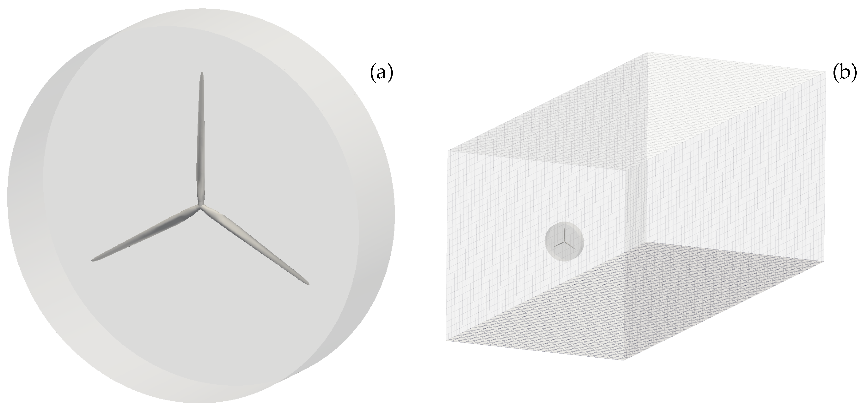
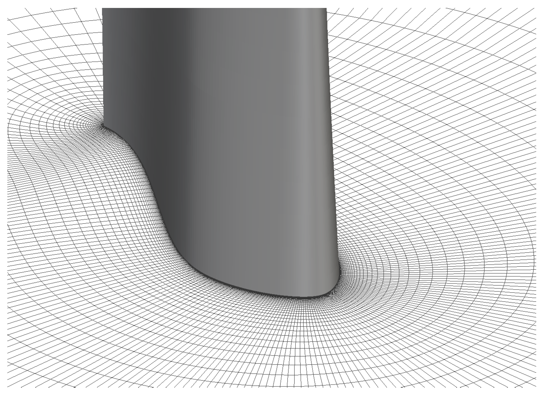
- BR: The blade resolved simulations are performed with the CFD software OpenFOAM V4.1 [8], which is an open-source package with a collection of modifiable libraries written in C++. The simulation domain is discretized using the bladeblockMesher [9] and windTurbine mesher tools [10] with a combination of structured and unstructured grids consisting of a total of 36M cells. To exclude influences of the mesh on the solution, a mesh study has been done in our previous work [11]. The grid of the complete simulation domain and the rotating part are shown in Figure 1 and a sectional view on the mesh near the blade in Figure 2. The cell length at the inlet, which is three rotor diameters upstream of the rotor, is 1m. This mesh is uniformly extruded up to the near blade mesh where a refinement takes place and the smallest cell length of approximately 0.2 m is reached. In order to limit the cell aspect ratio in radial direction, adaptive wall functions are being applied. The solution for the flow field is achieved by solving the incompressible Delayed Detached Eddy Simulations equations. It is assumed that the flow is fully turbulent, i.e., the laminar-turbulent transition in the boundary layer is not considered, because the inflow itself is turbulent and therefore the laminar boundary layer is not expected to have a strong influence on the blade. The closure problem is treated by use of the turbulence model proposed by Spalart et al. [12] with the proposed standard parameters. In order to solve the pressure-velocity coupling, the PIMPLE algorithm, is used, which is a combination of the loop structures of SIMPLE [13] and PISO [14]. Integration in time was performed using the implicit second order backward scheme together with the second order linear upwind scheme for discretizing the convection terms. For these simulations 360 cores were used for approximately 20 days resulting in 600 s simulation time with a time step of 0.01 s. This corresponds to 121 revolutions of the rotor.
- AL: The rotor is simplified by an AL model [6], where all rotor blades are reduced to rotating lines with a radial distribution of body forces at 60 positions along the lines. A Gaussian filtering kernel with the dimensionless smoothing parameter equal to 4 was used to obtain well fitting sectional forces and power output to the BR case. Based on the angle of attack at the given positions on the line, body forces are gained from lookup tables containing polars of two dimensional airfoils. A Prandtl tip [15] and root loss correction, as well as a 3D correction proposed by Du and Selig [16] are applied to the airfoil data. Except for a coarser resolution in the vicinity of the rotor with an average cell length of 1m the domain is exactly the same as for the BR case leading to a domain size of 22M cells. The flow field is simulated by Large Eddy Simulations (LES) with a Smagorinsky subgrid-scale model [17]. These simulations have been conducted on 360 cores for 25 h real time reaching 600 s simulation time with a time step of 0.01 s.
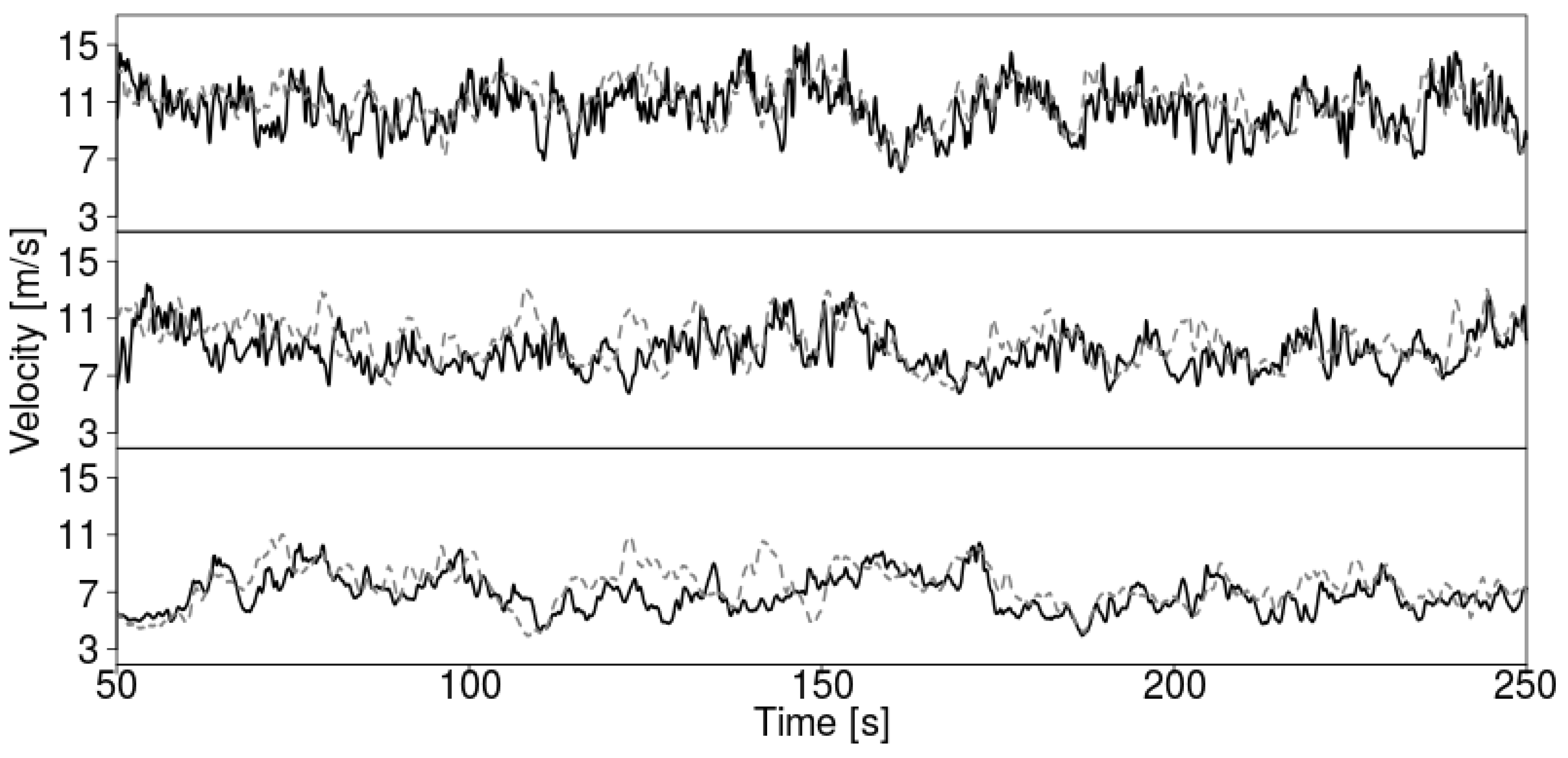
- BEM: This method uses wind fields recorded in the CFD domain on an equidistant 31 × 31 grid with a grid cell size of 4.5 m in both directions. In this case the fields are obtained at the position of the rotor from the same mesh as for the AL method but in an empty CFD domain. This seems to be a reasonable choice, because under this condition the TI at the rotor will be comparable for the CFD and BEM simulations. The BEM based tool FAST v8 [18] in combination with AeroDyn v15 [19] with the Beddoes Leishman type unsteady aerodynamics model [19,20] and an equilibrium wake model is used in this work. The BEM model relies on the very same airfoil data and correction models as the AL, but with only 17 blade sections. Because of the simplicity of the BEM approach the simulation with the same time stepping and total time as for the higher fidelity approaches only took two minutes on one core.
2.4. Fatigue Load Estimation
3. Results
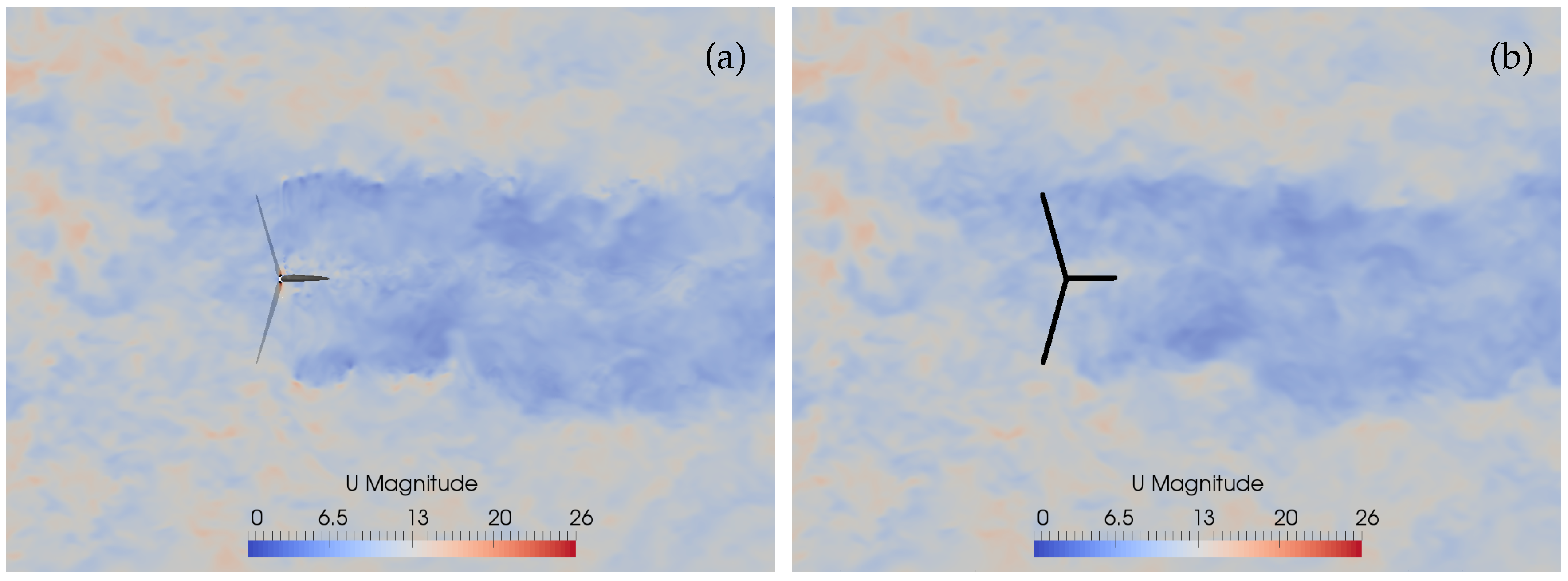
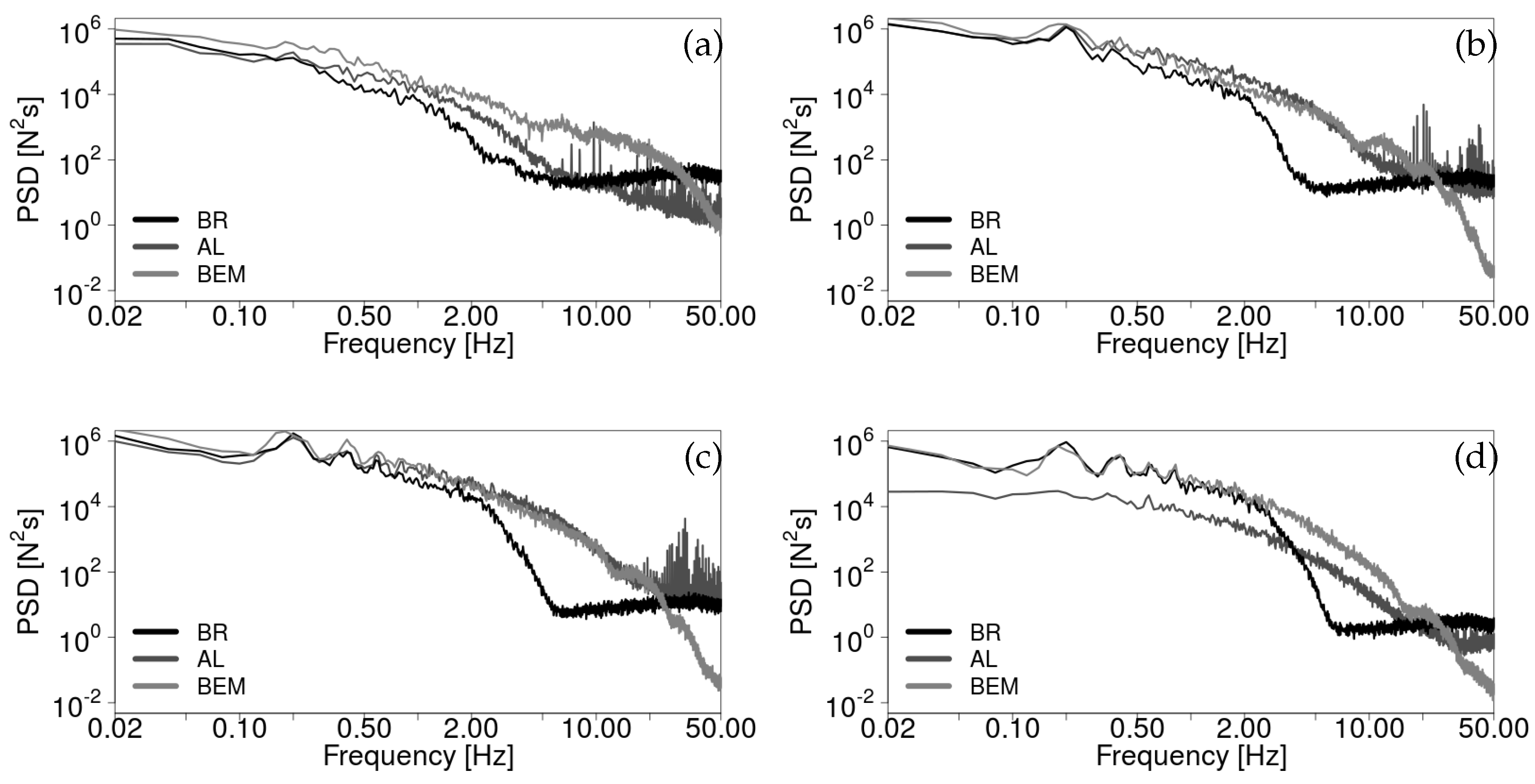
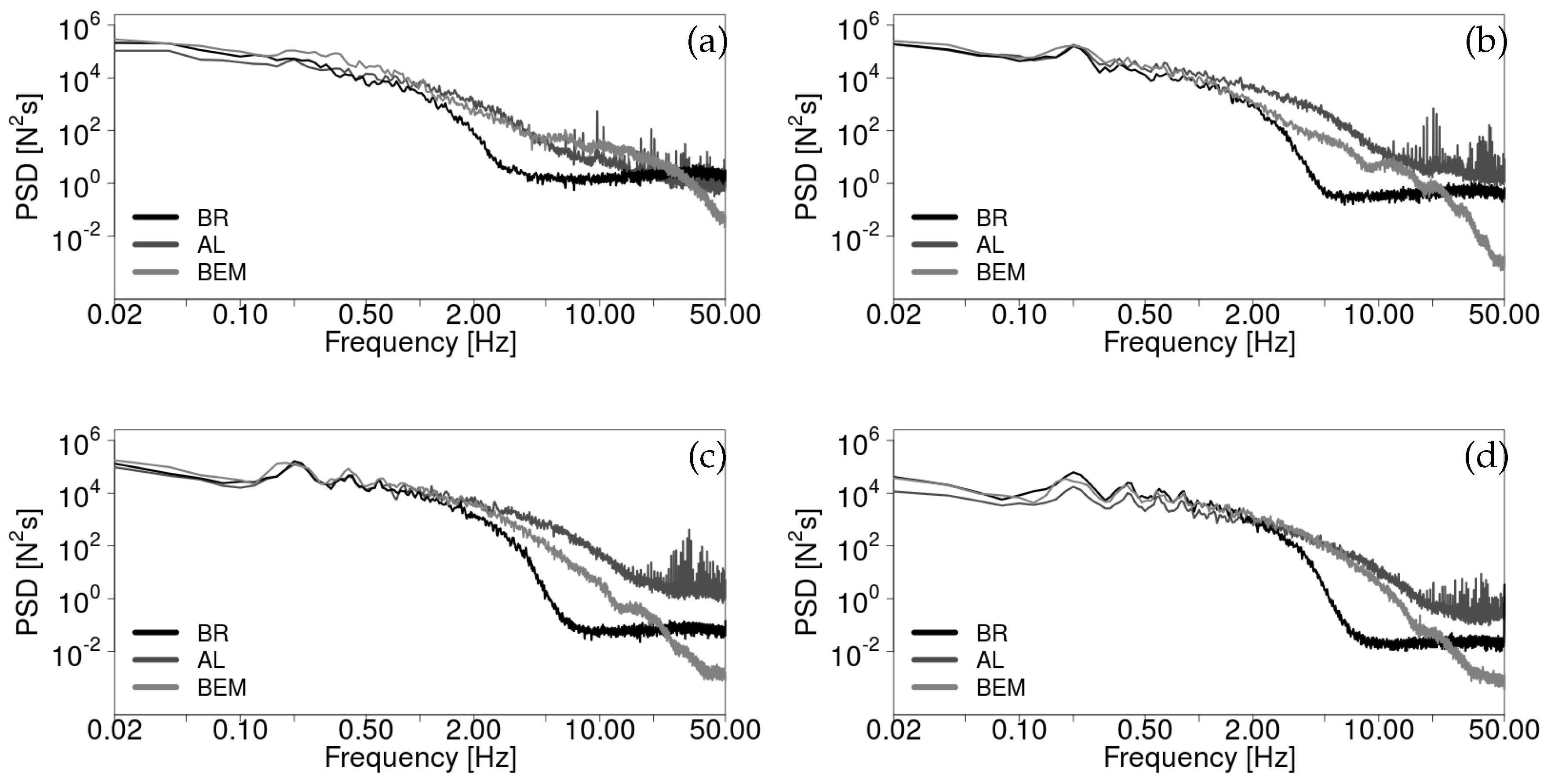
3.1. Wake Dynamics
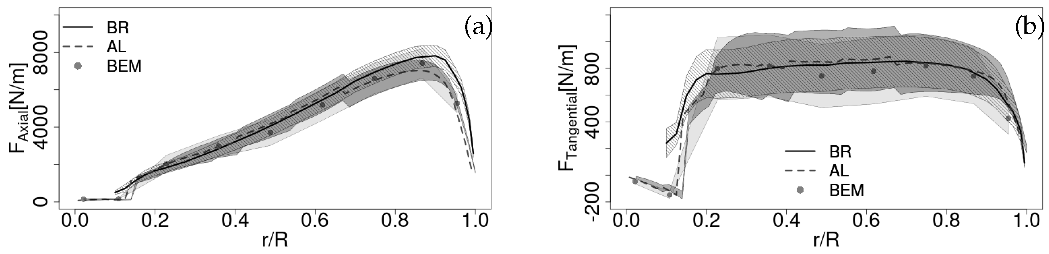
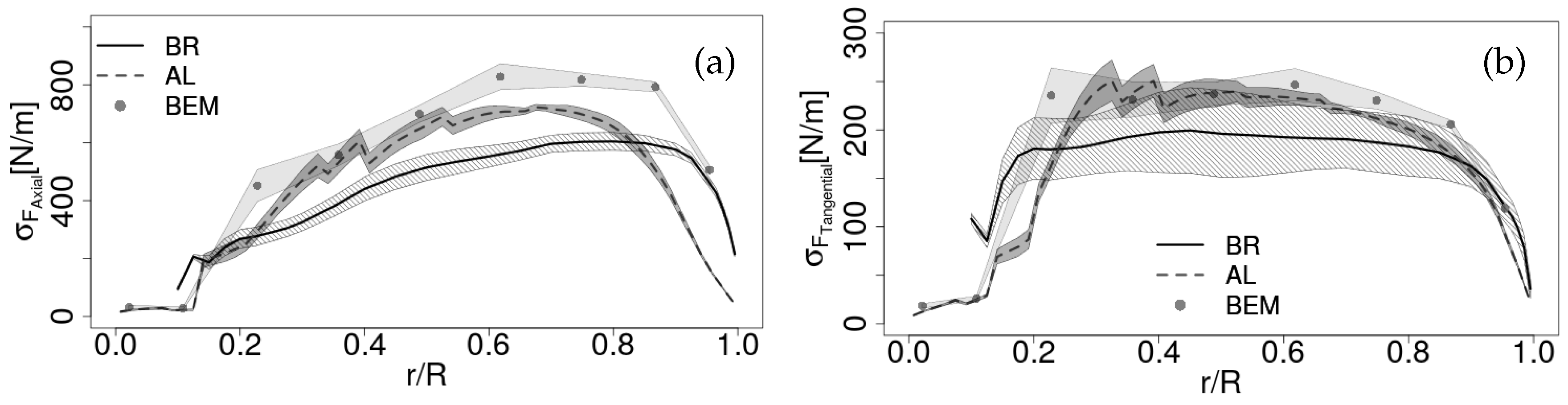
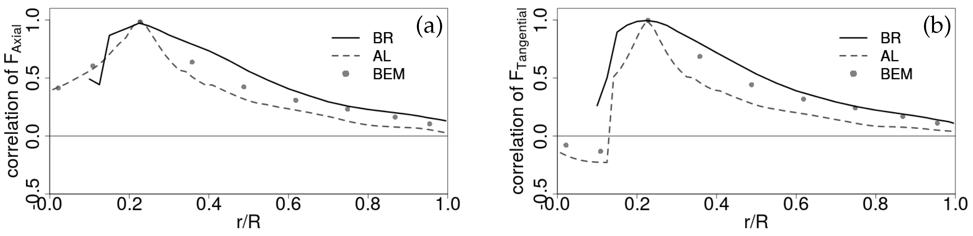
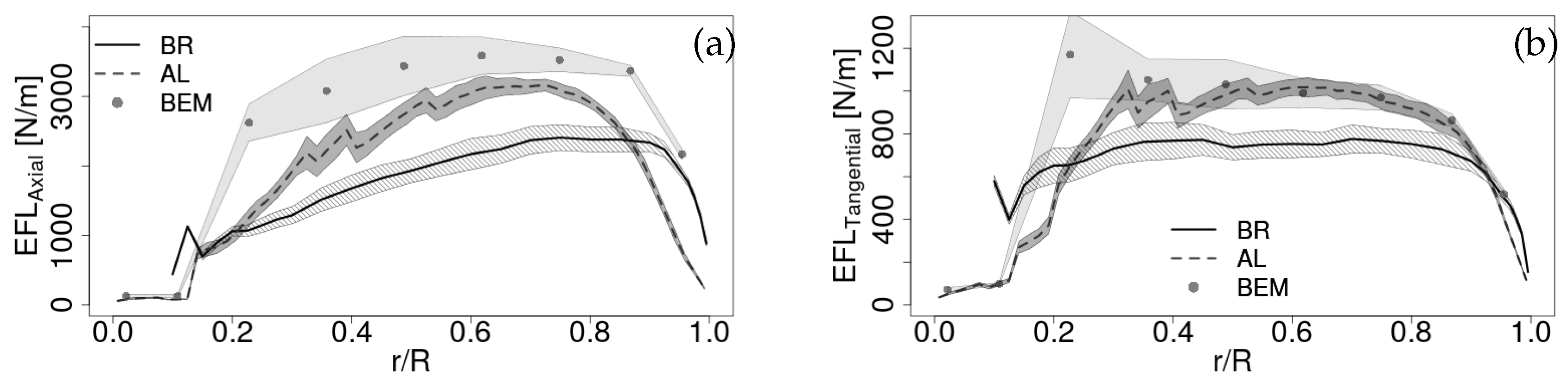
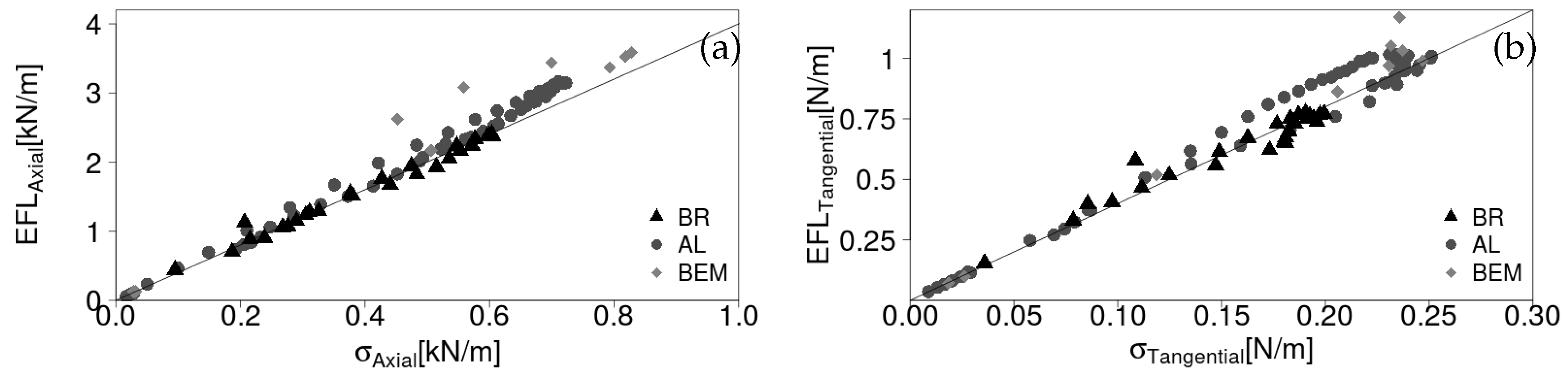
3.2. Sectional Forces
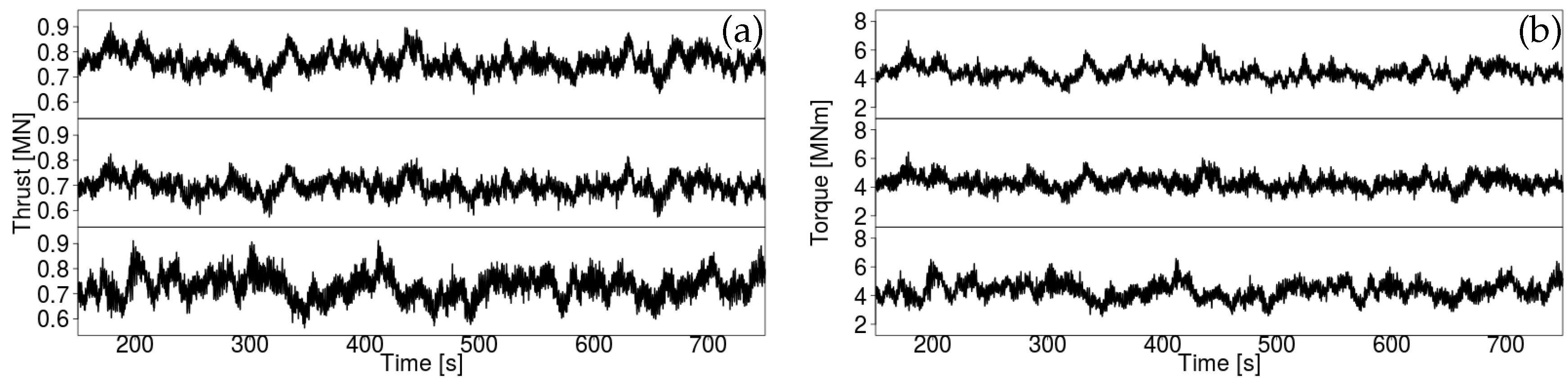
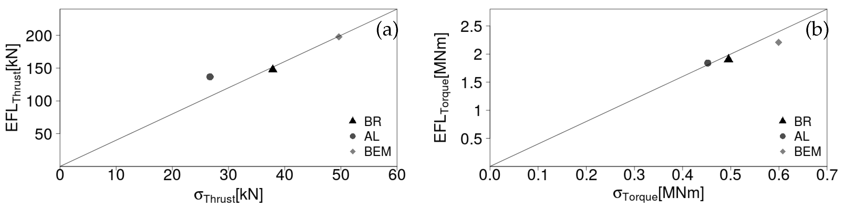
3.3. Integral Forces
4. Discussion
Author Contributions
Funding
Acknowledgments
Conflicts of Interest
Abbreviations
| AL | Actuator Line |
| BEM | Blade Element Momentum |
| BR | Blade Resolved |
| CFD | Computational Fluid Dynamics |
| EFL | Equivalent Fatigue Loads |
| PSD | Power Spectral Density |
| TI | Turbulence Intensity |
References
- Schepers, J.G. Engineering Models in Wind Energy Aerodynamics. Ph.D. Thesis, Delft University of Technology, Delft, The Netherlands, 2012. [Google Scholar]
- International Electrotechnical Commission. WIND TURBINES—PART 1: DESIGN REQUIREMENTS; Standard IEC 61400-1; International Electrotechnical Commission: Geneva, Switzerland, 2005. [Google Scholar]
- Madsen, H.A.; Sørensen, N.N.; Bak, C.; Troldborg, N.; Pirrung, G. Measured aerodynamic forces ona full scale 2MW turbine in comparison with EllipSys3D and HAWC2 simulations. J. Phys. Conf. Ser. 2018, 1037. [Google Scholar] [CrossRef]
- Kim, Y.; Lutz, T.; Jost, E.; Gomez-Iradi, S.; Muñoz, A.; Méndez, B.; Lampropoulos, N.; Sørensen, N.; Madsen, H.; van der Laan, P.; et al. AVATAR Deliverable D2.5: Effects of Inflow Turbulence on Large Wind Turbines. AVATAR Deliverable D2.5, Technical Report. Available online: http://www.eera-avatar.eu/fileadmin/avatar/user/avatar_D2p5_revised_20161231.pdf (accessed on 4 December 2018).
- Mann, J. Wind field simulation. Probabilistic Eng. Mech. 1998, 13, 269–282. [Google Scholar] [CrossRef]
- Sørensen, J.N.; Shen, W.Z. Numerical Modeling of Wind Turbine Wakes. J. Fluids Eng. 2002, 2002. 124, 393–399. [Google Scholar] [CrossRef]
- Jonkmann, J.; Butterfield, S.; Musial, W.; Scott, G. Definition of a 5-MW Reference Wind Turbine for Offshore System Development; Technical Report TP-500-38060; National Renewable Energy Laboratory: Golden, CO, USA, 2009.
- OpenCFD. OpenFOAM—The Open Source CFD Toolbox—User’s Guide; 1.4 ed.; OpenCFD Ltd.: Reading, UK, 2007. [Google Scholar]
- Rahimi, H.; Daniele, E.; Stoevesandt, B.; Peinke, J. Development and application of a grid generation tool for aerodynamic simulations of wind turbines. Wind Eng. 2016, 40, 148–172. [Google Scholar] [CrossRef]
- Rahimi, H. Validation and Improvement of Numerical Methods for Wind Turbine Aerodynamics. Ph.D. Thesis, University of Oldenburg, Oldenburg, Germany, 2018. [Google Scholar]
- Rahimi, H.; Garcia, A.M.; Stoevesandt, B.; Peinke, J.; Schepers, J.G. An engineering model for wind turbines under yawed conditions derived from high fidelity models. Wind Energy 2018, 21, 618–633. [Google Scholar] [CrossRef]
- Spalart, P.R.; Deck, S.; Shur, M.L.; Squires, K.D.; Strelets, M.K.; Travin, A. A New Version of Detached-eddy Simulation, Resistant to Ambiguous Grid Densities. Theor. Comput. Fluid Dyn. 2006, 20, 181. [Google Scholar] [CrossRef]
- Patankar, S.; Spalding, D. A calculation procedure for heat, mass and momentum transfer in three-dimensional parabolic flows. Int. J. Heat Mass Transfer 1972, 15, 1787–1806. [Google Scholar] [CrossRef]
- Issa, R. Solution of the implicitly discretised fluid flow equations by operator-splitting. J. Comput. Phys. 1986, 62, 40–65. [Google Scholar] [CrossRef]
- Prandtl, L. Ludwig Prandtl Gesammelte Abhandlungen: Zur Angewandten Mechanik, Hydro- und Aerodynamik; Springer: Berlin, Germany, 2013. [Google Scholar]
- Du, Z.; Selig, M. A 3-D stall-delay model for horizontal axis wind turbine performance prediction. In Proceedings of the 1998 ASME Wind Energy Symposium, Reno, NV, USA, 12–15 January 1998; p. 21. [Google Scholar]
- Smagorinsky, J. General Circulation Experiments with the Primitve Equations. Mon. Weather Rev. 1963, 91, 99–164. [Google Scholar] [CrossRef]
- Jonkman, B.; Jonkman, J. FAST v8.16.00a-bjj; Technical Report; NREL: Golden, CO, USA, 2016.
- Jonkman, J.; Hayman, G.; Jonkman, B.; Damian, R. AeroDyn v15 User’s Guide and Theory Manual (Draft Version); Technical Report; NREL: Golden, CO, USA, 2016.
- Leishman, J.G.; Beddoes, T.S. A Semi-Empirical Model for Dynamic Stall. J. Am. Helicopter Soc. 1989, 34, 3–17. [Google Scholar] [CrossRef]
- Madsen, P.H. Recommended Practices for Wind Turbine Testing and Evaluation. 3. Fatigue Loads; Riso National Laboratory: Roskilde, Denmark, 1990.
- Rychlik, I. A new definition of the rainflow cycle counting method. Int. J. Fatigue 1987, 9, 119–121. [Google Scholar] [CrossRef]
- Martínez-Tossas, L.A.; Churchfield, M.J.; Leonardi, S. Large eddy simulations of the flow past wind turbines: Actuator line and disk modeling. Wind Energy 2015, 18, 1047–1060. [Google Scholar] [CrossRef]


| Parameter | Value |
|---|---|
| Number of rotor blades | 3 |
| Rotor diameter | 126 m |
| Rated aerodynamic power | 5.3 MW |
| Rated wind speed | 11.4 m/s |
| Rated rotational speed | 12.1 rpm |
| Blade cone angle | 2.5 |
| Shaft tilt angle | 5.0 |
| Blade length | 61.5 m |
| Blade mass | 17,740 kg |
| BR | AL | BEM | AL/BR [%] | BEM/BR [%] | ||
|---|---|---|---|---|---|---|
| mean | 761 ± 7.3 | 698 ± 4.0 | 729 ± 9.6 | 91.7 | 95.8 | |
| Thrust [kN] | 37.9 ± 4.3 | 33.9 ± 2.6 | 49.7 ± 6.5 | 89.4 | 131.1 | |
| EFL | 147.6 ± 9.7 | 136.7 ± 4.2 | 190.1 ± 8.0 | 92.6 | 128.8 | |
| mean | 4.43 ± 0.10 | 4.32 ± 0.08 | 4.35 ± 0.13 | 97.5 | 98.2 | |
| Torque [MNm] | 0.495 ± 0.044 | 0.452 ± 0.038 | 0.599 ± 0.061 | 91.3 | 121.0 | |
| EFL | 1.90 ± 0.15 | 1.90 ± 0.13 | 2.29 ± 0.12 | 99.6 | 116.0 |
© 2018 by the authors. Licensee MDPI, Basel, Switzerland. This article is an open access article distributed under the terms and conditions of the Creative Commons Attribution (CC BY) license (http://creativecommons.org/licenses/by/4.0/).
Share and Cite
Ehrich, S.; Schwarz, C.M.; Rahimi, H.; Stoevesandt, B.; Peinke, J. Comparison of the Blade Element Momentum Theory with Computational Fluid Dynamics for Wind Turbine Simulations in Turbulent Inflow. Appl. Sci. 2018, 8, 2513. https://0-doi-org.brum.beds.ac.uk/10.3390/app8122513
Ehrich S, Schwarz CM, Rahimi H, Stoevesandt B, Peinke J. Comparison of the Blade Element Momentum Theory with Computational Fluid Dynamics for Wind Turbine Simulations in Turbulent Inflow. Applied Sciences. 2018; 8(12):2513. https://0-doi-org.brum.beds.ac.uk/10.3390/app8122513
Chicago/Turabian StyleEhrich, Sebastian, Carl Michael Schwarz, Hamid Rahimi, Bernhard Stoevesandt, and Joachim Peinke. 2018. "Comparison of the Blade Element Momentum Theory with Computational Fluid Dynamics for Wind Turbine Simulations in Turbulent Inflow" Applied Sciences 8, no. 12: 2513. https://0-doi-org.brum.beds.ac.uk/10.3390/app8122513