An Image Segmentation Method Using an Active Contour Model Based on Improved SPF and LIF

Abstract

Inhomogeneous images cannot be segmented quickly or accurately using local or global image information. To solve this problem, an image segmentation method using a novel active contour model that is based on an improved signed pressure force (SPF) function and a local image fitting (LIF) model is proposed in this paper, which is based on local and global image information. First, a weight function of the global grayscale means of the inside and outside of a contour curve is presented by combining the internal gray mean value with the external gray mean value, based on which a new SPF function is defined. The SPF function can segment blurred images and weak gradient images. Then, the LIF model is introduced by using local image information to segment intensity-inhomogeneous images. Subsequently, a weight function is established based on the local and global image information, and then the weight function is used to adjust the weights between the local information term and the global information term. Thus, a novel active contour model is presented, and an improved SPF- and LIF-based image segmentation (SPFLIF-IS) algorithm is developed based on that model. Experimental results show that the proposed method not only exhibits high robustness to the initial contour and noise but also effectively segments multiobjective images and images with intensity inhomogeneity and can analyze real images well.

1. Introduction

Image segmentation is an important task in the field of image analysis and object detection and aims to segment an image into distinctive subregions that are meaningful to analyze [1]. Segmentation is the intermediate step between image processing and image analysis as well as the bridge from low- to high-level research in computer vision. Inhomogeneity, noise, and low contrast in real images have increased the difficulty of image segmentation [2].

Over the past few decades, many segmentation methods have been proposed. The active contour model (ACM), which was proposed by Kass et al. [3], has been proven to be an efficient framework for image segmentation. The fundamental idea of the ACM framework is to control a curve to move toward its interior normal and then stop on the true boundary of an object based on an energy minimization model [4]. The two main shortcomings of ACM algorithms are (1) sensitivity to the initial position and (2) difficulties related to topological changes [5]. Generally, existing ACM methods can be roughly divided into the following types, edge-based models [6,7,8,9] and region-based models [10,11,12,13,14].

The geodesic active contour (GAC) model [15] is the most typical of edge-based methods. Owing to the edge-indicator function, the model can stop at high-contrast image gradients [16]. Edge-based models have distinct disadvantages. For example, these methods can effectively segment an object with strong edges; however, they cannot detect the weak edges of an object. Moreover, the methods are sensitive to noise and do not easily obtain satisfactory segmentation results for blurred images [2]. In addition, the contour should initially be set near the object; otherwise, it is difficult to obtain correct segmentation results [17]. Region-based models make full use of image statistical information, whereas edge-based models do not. Thus, region-based models have multiple advantages over edge-based models. For example, because regional information is used, region-based models are less sensitive to contour initialization and noise. Furthermore, these region-based models can easily segment images with weak boundaries or even those without boundaries [18]. One of the most typical region-based methods was proposed by Chan and Vese (C–V) [11], which is based on the Mumford–Shah functional [19]. The C–V model is based on the assumption that image intensities are homogeneous in each region. However, this assumption does not suit the intensity of inhomogeneous images, which limits the method’s further applications [20,21].

Recently, hybrid methods have gained popularity among region-based methods. These methods combine region (local or global) and edge information in their energy formulations [22]. Zhang et al. [23] proposed the selective binary and Gaussian filtering regularized level set (SBGFRLS) model. This model combines the advantages of region-based and edge-based active contours and introduces a region-based SPF function, which utilizes the image global intensity means from the C–V method. This method adopts an approach similar to that of the GAC model. However, the edge-indicator function is replaced with a region-based SPF function in the model. Moreover, the traditional regularization function is usually replaced with a Gaussian smoothing function. This traditional method uses only global image intensity information. Therefore, the method is unable to analyze intensity-inhomogeneous images [21,22]. Li et al. [24] investigated a local binary fitting (LBF) model, which is an efficient region-based level set method. The LBF model introduces a local binary fitting energy with a kernel function and uses the intensity of the current pixel to approximate the intensities of the neighboring pixels to obtain accurate segmentation performance; the model can be used to address intensity-inhomogeneous images and has attracted extensive attention due to its satisfactory segmentation performance [25]. However, this model involves high computational complexity. In addition, the model is sensitive to the initialization location and parameters [5,26]. Wang et al. [27] defined an energy functional that combines the merits of the C–V model and the LBF model [21]. Because the new model employs local and global intensity information, it can avoid becoming trapped in a local minimum; however, the result remains partially dependent on the initialization location [21]. Zhang et al. [28] exploited a local image region statistics-based improved ACM method (LSACM) in the presence of intensity inhomogeneity. The LSACM is robust to noise while suppressing intensity overlap to some extent. Yuan et al. [25] offered a model based on global and local regions. The global term takes gradient amplitude into consideration, and the local term adopts local image information by convolving the Gaussian kernel function [29]. This algorithm is sensitive to the initialization location because of the use of gradient information. Similarly, Zhao et al. [30] adopted local region statistical information and gradient information to construct an energy functional and faced the same problem. Zhang et al. [31] introduced a local image fitting (LIF) energy functional to extract local image information and proposed a Gaussian filtering method for a variational level set to regularize the level set function, which can be interpreted as a constraint on the differences between the original image and the fitting image [12,24]. Furthermore, the method used Gaussian kernel filtering to regularize the level set function, and a reinitialization operation was avoided [32]. Unfortunately, the abovementioned methods are sensitive to initialization, and they are also unable to analyze images with intensity inhomogeneity. Hence, these limitations obviously limit their practical applications. Here, we focus on overcoming these drawbacks in this paper.

In this study, to segment the images quickly and accurately, a new image segmentation model is proposed based on an improved SPF and LIF. This method defines a new SPF function, which uses global image information, and the SPF function can segment blurred images and weak gradient images. Then, the LIF model is introduced, which is based on local image information, and this model is used to segment intensity-inhomogeneous images. Moreover, a weight function is established to adjust the weights between the SPF model and the LIF model. Thus, a novel ACM model is presented, and an image segmentation algorithm is investigated. Experimental results demonstrate that our model involves simpler computation, exhibits faster convergence, and can effectively segment multiobjective images and intensity-inhomogeneous images. Furthermore, the proposed method is highly robust to the initial contour and noise.

The remainder of this paper is structured as follows. Section 2 briefly reviews the GAC, C–V, SBGFRLS, and LIF models. In Section 3, by combining the improved SPF function with the LIF model, a novel ACM is presented, and using this model, an image segmentation algorithm is designed. Then, the experimental results and analysis are discussed in Section 4. Section 5 presents the conclusions.

2. Related Work

2.1. The GAC Model

The GAC model uses image gradient information from the boundary of an object [33]. Suppose that I: Ω$\subset$R² is an image domain, I: Ω → R² is an input image, and C(q) is a closed curve. Then, the GAC model is formalized by minimizing the following energy functional as

$$E^{GAC}={\displaystyle {\int }_0^{1}g(|\nabla I(C(q))|)}|C’(q)|dq,$$

(1)

where g is a strictly decreasing function.

Usually, a satisfactory edge stopping function (ESF) should be defined, which is regular and positive at object boundaries [21], e.g.,

$$g(|\nabla I|)=\frac{1}{1+|\nabla G_{\sigma }\ast I{|}^2},$$

(2)

where G_σ denotes the Gaussian kernel function and G_σ*I describes the convolution operation of I with G_σ.

Using the steepest descent method and the calculus of variations, we obtain the Euler–Lagrange form of Equation (1), which is written as

$$C_t=g(|\nabla I|)k\overrightarrow{N}-(\nabla g\cdot \overrightarrow{N})\overrightarrow{N},$$

(3)

where k is the curvature of the contour and $\overrightarrow{N}$ is the inward normal to the curve. A constant velocity term α is typically added to increase the propagation speed [21]. Thus, Equation (3) can be rewritten as

$$C_t=g(|\nabla I|)(k+\phi )\overrightarrow{N}-(\nabla g\cdot \overrightarrow{N})\overrightarrow{N}.$$

(4)

The corresponding level set formulation is described as

$$\frac{\partial \phi }{\partial t}=g|\nabla \phi |(div(\frac{\nabla \phi }{|\nabla \phi |})+\alpha )+\nabla g\cdot \nabla \phi ,$$

(5)

where ϕ represents the level set function and α is the balloon force that controls the shrinkage or expansion of the contour.

The GAC model utilizes the image gradient to construct an ESF, which can stop the contour evolution on object boundaries. When images have weak boundaries or the initial contour is far from the desired object boundary, the GAC model will fail to find the target [18,22].

2.2. The C–V Model

The C–V model is proposed based on the assumption that the original image intensity is homogeneous. The energy functional of the C–V model [34] is expressed as

$$E^{CV}={\lambda }_1{{\displaystyle {\int }_{inside(c)}|I(x)-c_1|}}^{2}dx+{\lambda }_2{{\displaystyle {\int }_{outside(c)}|I(x)-c_2|}}^{2}dx,$$

(6)

where λ₁ and λ₂ are positive constants that regulate image driving force inside and outside the contour, c₁ represents the mean gray value of the target area and the background area in the evolution curve C, and c₂ represents the mean gray value of the target area and the background area outside the evolution curve C.

By minimizing Equation (6), one has c₁ and c₂, which are described, respectively, as

$$c_1=\frac{{\displaystyle \int I(x)H(\phi (x))dx}}{{\displaystyle \int H(\phi (x))dx}},$$

(7)

$$c_2=\frac{{\displaystyle \int I(x)(1-H(\phi (x)))}dx}{{\displaystyle \int (1-H(\phi (x)))dx}},$$

(8)

where H(ϕ) is the Heaviside function.

In practice, the Heaviside function H(ϕ) and the Dirac delta function δ(ϕ) must be approximated by smooth functions H_ε(ϕ) and δ_ε(ϕ) when ε$\to$0, which are typically expressed as follows, respectively

$$H_{\epsilon }(x)=\frac{1}{2}[1+\frac{2}{\pi }\arctan (\frac{x}{\epsilon })],$$

(9)

$${\delta }_{\epsilon }(x)=\frac{1}{\pi }\cdot \frac{\epsilon }{{\epsilon }^2+x^2},$$

(10)

By incorporating the length and area energy terms into Equation (6) and further minimizing the length and area of the level set curve, the corresponding partial differential equation is described as

$$\frac{\partial \phi }{\partial t}=\delta (\phi )\left[\mu \nabla (\frac{\nabla \phi }{|\nabla \phi |})-v-{\lambda }_1{|I-c_1|}^2+{\lambda }_2{|I-c_2|}^2\right],$$

(11)

where μ, ν, λ₁, and λ₂ denote the corresponding coefficients, all of which are positive constants; $\nabla$ is the gradient operator; μ controls the smoothness of the zero level set; ν increases the propagation speed; and λ₁ and λ₂ control the image data driving force inside and outside the contour, respectively.

Because c₁ and c₂ are related to the global information inside and outside the curve, this model can segment blurred images and images with weak gradients more effectively than the edge-based model can, and it is insensitive to the initialization location [22,35]. However, when the internal and external intensities of the curve are inhomogeneous, c₁ and c₂ cannot express the local information precisely, which leads to the failure of image segmentation [2].

2.3. The SBGFRLS Model

The SBGFRLS model is proposed based on the traditional C–V model and the GAC model, thereby seizing the advantages of both models [21]. In the SBGFRLS model, an SPF function is used to substitute ESF in the GAC model, and thus the level set formulation of the SBGFRLS can be expressed as

$$\frac{\partial \phi }{\partial t}=spf(I(x))\cdot (div(\frac{\nabla \phi }{|\nabla \phi |})+\alpha )|\nabla \phi |+\nabla spf(I(x))\cdot \nabla \phi ,$$

(12)

where spf(I(x)) in Equation (12) is an SPF function, which can be given as

$$spf(I(x))=\frac{I(x)-\frac{c_1+c_2}{2}}{\max (|I(x)-\frac{c_1+c_2}{2}|)},$$

(13)

where c₁ and c₂ represent the gray mean values of regions outside and inside the contour, computed using Equations (7) and (8), respectively.

The SBGFRLS model can reduce the cost of the expensive reinitialization of the traditional level set method and is more efficient than traditional models. The model stops the contour evolution, even with blurred edges, without any a priori training. However, the model assumes that the region to be segmented is homogeneous. This assumption occasionally holds in general clinical cases. When facing heterogeneous intensity distributions, the detection accuracy can fall significantly because the fundamental assumption is violated [36,37]. Moreover, the SBGFRLS model can become trapped in a local minimum without proper initialization, which leads to poor segmentation performance [38,39,40].

2.4. The LIF Model

The local fitted image (LFI) formulation [31] is defined based on local image information, based on which the LIF model is investigated. This model can segment intensity-inhomogeneous images [41]. The LIF model is expressed as follows

$$E^{LIF}(\phi )=\frac{1}{2}{\displaystyle {\int }_{\mathsf{\Omega }}|I(x)-I^{LFI}(x){|}^2}dx,$$

(14)

where I^LFI is a local fitted image, and any $x\in \mathsf{\Omega }$.

It follows that I^LFI can be calculated as

$$I^{LFI}(x)=m_1{H}_{\epsilon }(\phi )+m_2(1-H_{\epsilon }(\phi )),$$

(15)

where m₁ and m₂ are expressed, respectively, as

$$\{\begin{array}{l}{m}_1=mean(I\in (\{x\in \mathsf{\Omega }|\phi (x)>0\}\cap W_k(x)))\\ m_2=mean(I\in (\{x\in \mathsf{\Omega }|\phi (x)<0\}\cap W_k(x)))\end{array},$$

(16)

ϕ is the zero level set of a Lipschitz function that represents the contour C; H_ε(ϕ) is the regularized Heaviside function, as defined in Equation (9); and W_k (x) is a rectangular window function.

In our experiment, W_k (x) is a truncated Gaussian window with a standard deviation of $\sigma$ and size (4k + 1) × (4k + 1), where k is the greatest integer that is smaller than $\sigma$. Similarly, the segmentation results can be achieved if a constant window is chosen [31].

According to the calculus of variations and the gradient descent method, the following partial differential equation can be obtained by minimizing E^LIF:

$$\frac{\partial \phi }{\partial t}=(I-I^{LFI})(m_1-m_2){\delta }_{\epsilon }(\phi ),$$

(17)

where δ_ε(ϕ) is the regularized Dirac delta function [32], which is calculated as indicated in Equation (10).

According to the complexity analysis and experimental results in [31,32,41,42], the LIF model is more efficient than the LBF model. However, neither model can handle noisy and intensity-inhomogeneous images well [41,42].

3. Proposed Method

3.1. Improved SPF Function

The main strategy of the ACM based on region information is to construct a driving force, which is based on the information of the image region [43]. The region function modulates the sign of the pressure forces using region information such that the contour shrinks when it is outside the object of interest and expands when it is inside the object. For this reason, these external forces are sometimes called SPF [43]. Zhang et al. [22] proposed the SBGFRLS model, which utilizes the statistical information inside and outside the contour to construct a region-based SPF function [37]. However, an SPF function is simply based on image information. Thus, the corresponding model cannot segment intensity-inhomogeneous images or images with weak boundaries [36,41].

In this study, the global information of image I is used to divide the image into two parts, inC and outC, and the level set function is then introduced into the new SPF function.

Using global region information and combining c₁ and c₂, a global fitted image formulation is defined as

$$f=H_{\epsilon }(\phi ).*(I-c_1)+(1-H_{\epsilon }(\phi )).*(I-c_2),$$

(18)

where H_ε(ϕ) defined in Equation (9) is the regularized Heaviside function and c₁ and c₂ are calculated by Equations (7) and (8), respectively, and $.*$ describes matrix multiplication.

By employing the above-defined global fitted image, a new SPF function is defined as

$$spf(I(x))=\frac{I(x)-f(x)}{\max (|f(x)|)}.$$

(19)

According to the construction approach of the SPF function, a new partial differential equation is defined as

$$\frac{\partial \phi }{\partial t}=spf(I(x))\cdot \alpha ,$$

(20)

where α is the balloon force that controls the shrinkage or the expansion of the contour. In this paper, according to the concept of a balloon force established previously [44], a balloon force is reconstructed to change the evolution rate of the level set function adaptively, which is defined as

$${\alpha }_{new}=c_1+c_2.$$

(21)

The new SPF is more efficient than the traditional ACM models because this function avoids the expensive cost of the reinitialization step. Moreover, the SPF is less sensitive to the initialization location. However, the SPF function is constructed with only global image information. Therefore, it appears difficult to handle images with intensity inhomogeneity using this approach.

3.2. Active Contour Model Based on Improved SPF and LIF

Zhang et al. [31] constructed the LIF model, which can effectively process nonhomogeneous images through local image information. Unfortunately, the model is sensitive to the initial curve and noise [2]. To construct a model that can process nonhomogeneous images and reduce the dependence on the location of the initial contour, this subsection combines the new SPF function with the existing LIF model to form a new ACM based on local and global image information.

By combining the new SPF function with the LIF model, the new level set evolution equation is defined as

$$\frac{\partial \phi }{\partial t}=\lambda (I-I^{LIF})(m_1-m_2){\delta }_{\epsilon }(\phi )+(1-\lambda )spf(I(x))\cdot \alpha ,$$

(22)

where δ_ε(ϕ), defined in Equation (10), is the regularized Dirac delta function and λ is a new weight coefficient.

Here, λ is a weight function that can be employed to dynamically adjust the ratio between the local and the global term in image segmentation. Namely, the image information term playing a crucial role in segmenting an image can be selected.

Based on the local and global image information, the weight coefficient λ is defined as

$$\lambda =\frac{A}{\max (|B|)},$$

(23)

where A is defined in Equation (21) and B is defined as

$$B=m_1+m_2,$$

(24)

where m₁ and m₂ are defined in Equation (16).

It is noted that the selection of the weight parameter λ is important in controlling the influence of the local and the global terms. Li et al. [45] declared that the local term is critical to the initialization to some extent; a global term is incorporated into the local framework, thereby forming a hybrid ACM. Therefore, with the mutual assistance of the local force and the global force, the robustness to the initialization can be improved, and the global force is dominant if the evolution curve is away from the object. When the contour is placed near the object boundaries, the LIF model plays a dominant role, and fine details can be detected accurately. In contrast, the new SPF model plays a key role when the contour is located far from the object boundaries, and owing to the assistance of the SPF, a flexible initialization is allowed. It follows that the automatic adjustment between the LIF and SPF models in our ACM is very distinct. Furthermore, the objective of the dynamic adjustment is to determine an optimal result for image segmentation.

In general, the new proposed SPFLIF-IS model not only solves the problem that the intensity-inhomogeneous images cannot be accurately segmented by using the global image information but also overcomes the primary shortcoming that the model based on the local image information is sensitive to noise and the initial contour.

3.3. Algorithm Steps

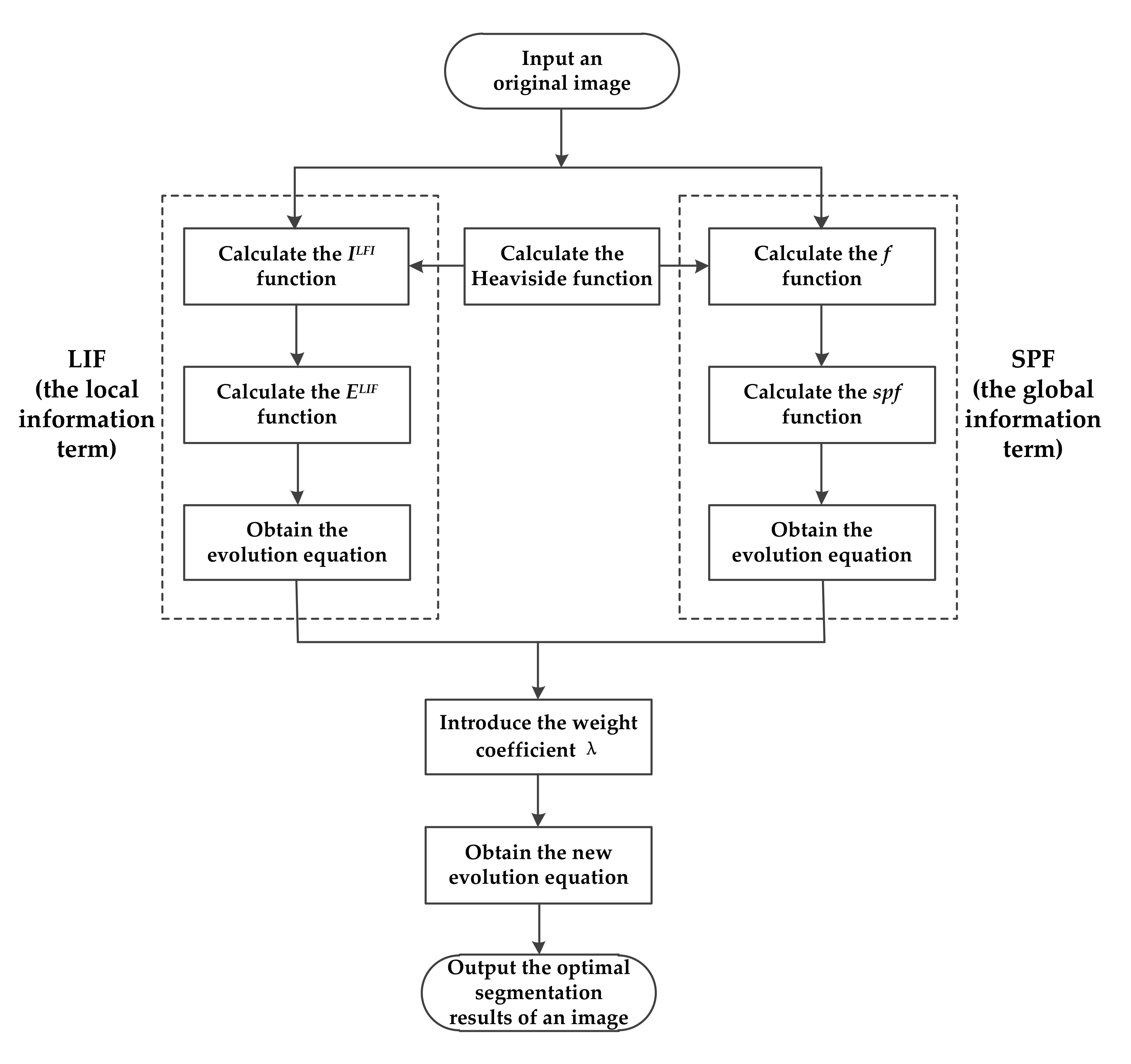
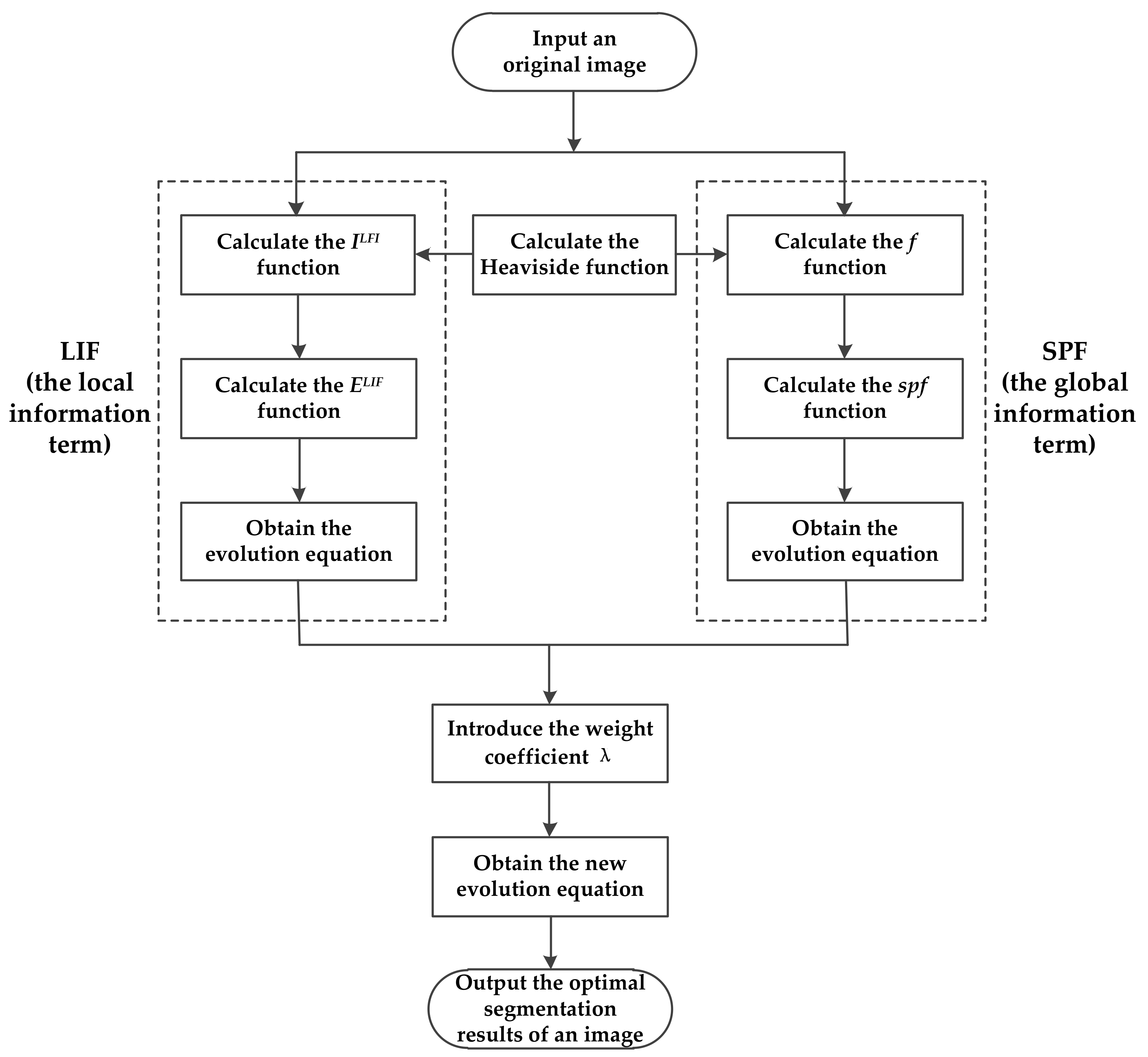
The procedures of image segmentation are illustrated in Figure 1.

After the abovementioned image segmentation algorithm has been applied, an improved SPF and LIF-based image segmentation (SPFLIF-IS) algorithm using ACM can be implemented and described as Algorithm 1, which is summarized as follows.

Algorithm 1. SPFLIF-IS

Input: An original image

Output: The result of image segmentation Step 1: Initialize the level set function ϕ, and set the coefficients Δt, n, and ε. Step 2: Calculate the Heaviside function and the Dirac delta function using Equations (9) and (10), respectively. Step 3: Forn = 1: iterNum // iterNum is the total number of iterations. Step 4: Compute c1 and c2 by Equations (7) and (8), respectively, and obtain f according to Equation (18). Step 5: Calculate spf(I(x)), according to Equation (19), and obtain the level set evolution equation by Equation (20). Step 6: Introduce the LIF model. Step 7: Calculate the weight coefficient λ using Equation (23). Step 8: Calculate the level set evolution equation using Equation (22). Step 9: If the evolution of the curve is stable, then output the segmentation result. Else, return to Step 4. Step 10: End for

It is well known that convolution operations are the most time-consuming with respect to the time complexity of an algorithm. Therefore, it is necessary to explain the complexity of the convolution operation. When an algorithm requires a convolution operation, the time cost is approximately O(n² × N) [46], where N is the image size and n is the Gaussian kernel. The values of N are greater than n².

Because the C–V model [34] must be reinitialized in every iteration, its time cost is very high, and the computational complexity is O(N²) [31]. The LBF model [24] usually needs to perform four convolution operations in each iteration, which greatly increases the computational time complexity. This situation indicates that the time complexity is O(itr × 4 × n² × N), where the parameter itr is the number of iterations. In contrast, the SBGFRLS model [23] must perform three convolution operations, two of which are derived by gradient calculation (horizontal and vertical), and the other involves mask image and filter mask. Thus, the total computational complexity of the SBGFRLS model is O(itr × 3 × n² × N). The LIF model [31] performs two convolution operations in each iteration. Thus, the total computational time required for the LIF model is O(itr × 2 × n² × N). For the SPFLIF-IS algorithm, the computational complexity is mainly concentrated in Step 6. In Algorithm 1, Step 6 is the most time-consuming to calculate in the LIF model. The computational complexity of our proposed method is O(itr × 2 × n² × N), where n is the size of the Gaussian kernel function and N is the image size. Since in most cases, N >> n², the complexity of SPFLIF-IS is O(N) approximately, which is close to that of the LIF model in [31]. It follows that our proposed method is much more computationally efficient than the C–V model [31], the LBF model [24], and the SBGFRLS model [23]. Because the SPFLIF-IS algorithm decreases the number of Gaussian convolution operations required, its time costs and number of iteration operations are drastically reduced. Therefore, the computational complexity of our SPFLIF-IS method is lower than that of the other related ACMs [6,8,11,12,15,17,20,23,24,31,34,43].

4. Experimental Results

4.1. Experiment Preparation

In this section, comprehensive segmentation results for all algorithms compared are presented to validate the performance of our proposed method on various representative synthetic and real images with respect to different characteristics. Following the experimental techniques for image segmentation designed by Ji et al. [42], these selected images are mostly corrupted with one or more degenerative characteristics, including additive noise, low contrast, weak edges, and intensity inhomogeneity. Unless otherwise specified, the same parameters are employed as follows, Δt = 1, n = 5, ε = 1.5, and ${\phi }_0\left(x, y\right) = 1: (x, y)\in \mathrm{in}\left(c\right)$ or ${\varphi }_0\left(x, y\right) = -1: (x, y)\in \mathrm{out}\left(c\right)$. The Gaussian kernel plays an important role in practical applications; the kernel is a scale parameter controlling region scalability from small neighborhoods to the entire image domain [31]. In general, the value of the scale parameter should be appropriately selected from practical images. It is well known that an excessively small value may cause undesirable results, whereas an excessively large value can lead to high computational complexity [31,36]. Thus, the Gaussian kernel size controlling the regularization of the level set function should be chosen according to practical cases [36]. Following the experimental techniques designed in [31,36], the σ selected in our experiments is typically less than 10. All of models compared in this paper are tested in MATLAB R2014a in a Windows 7 environment using a 3.20 GHz Intel (R) Core i5-3470M processor with 4 GB RAM.

4.2. Segmentation Results of Images with Intensity Inhomogeneity

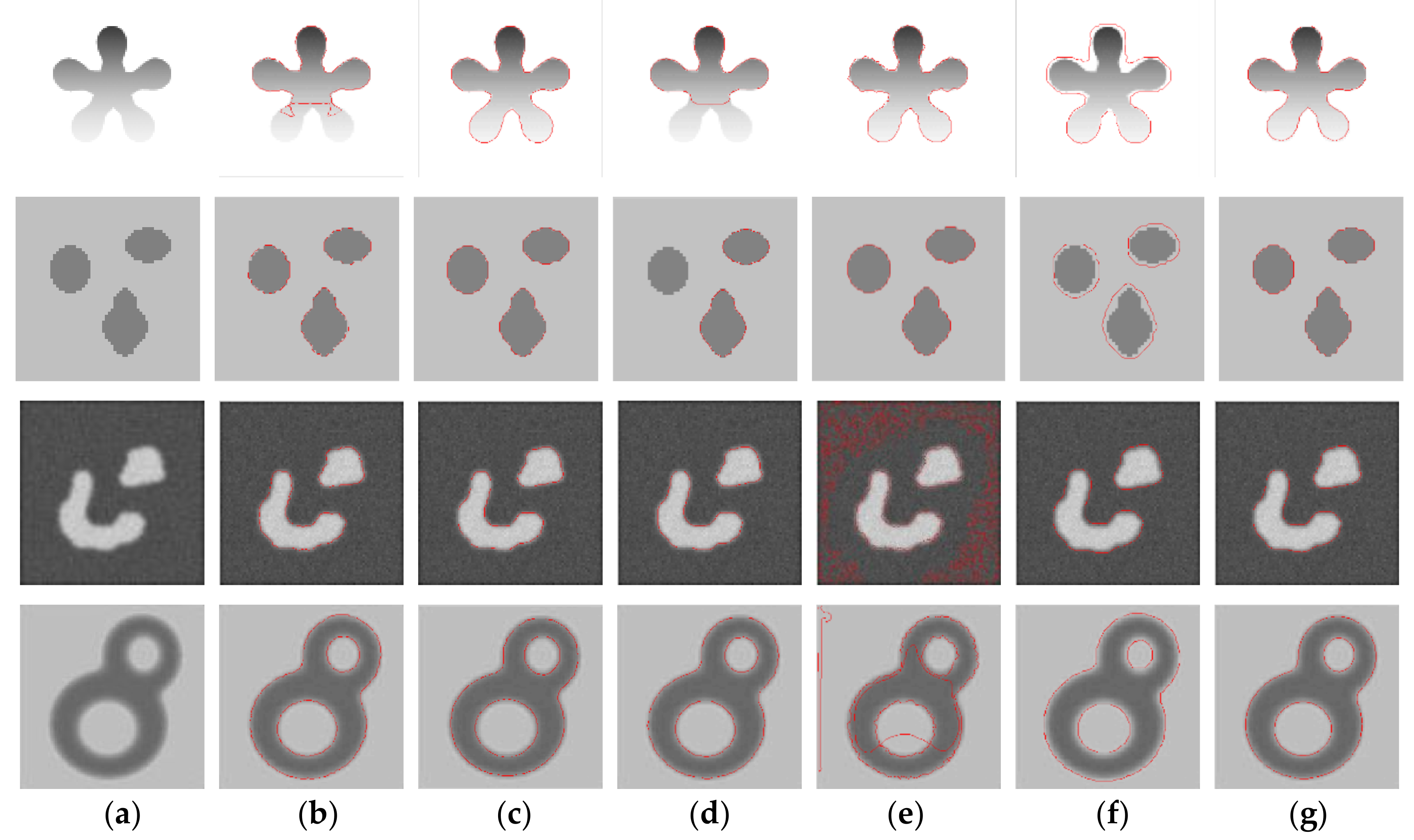
To demonstrate the satisfactory performance and effectiveness of the SPFLIF-IS model, a series of experimental results are presented. We compare our model with the following five existing models: (1) the C–V (The code is available at [47]) model [34], (2) the LBF (The code is available at [48]) model [24], (3) the LIF (The code is available at [47]) model [31], (4) the SBGFRLS (The code is available at [47]) model [23], and (5) the LSACM model [28]. The five representative ACM algorithms are the state-of-the-art level set methods published recently for image segmentation. The algorithms show improvements over the classical ACM and are specially selected based on the level set method for comparison experiments. The chosen parameters for these models can be found in [23,24,28,31,34]. The segmentation results obtained for images with intensity inhomogeneity using the six models are illustrated in Figure 2, where the original images shown in Figure 2a can be found in [2].

Figure 2b,d,f shows that the C–V model, the SBGFRLS model, and the LSACM model fail to analyze the first image with intensity inhomogeneity. As shown in Figure 2d,f, the SBGFRLS model and the LSACM cannot yield the ideal segmentation results for the second image. The object boundaries of the third image are not identified by the LIF model, and the results are shown in Figure 2e. Figure 2e,f shows that the true boundaries of the fourth image are not accurately extracted by the LIF model or the LSACM model. The SPFLIF-IS model detects the true boundary, and the results are illustrated in Figure 2g. Meanwhile, Figure 2c,g shows that the LBF model perform as well as the SPLIF-IS model.

Note that because the visual evaluations in Figure 2 are partial to subjective measures, to strengthen the objective results of our experiments, the corresponding tables should be added to defend the arguments for all the tested images in the following visual evaluations, in which each failure is clearly labeled to avoid ambiguity. To more clearly illustrate this state, the following symbols are adopted in the tables: F1: fail to detect boundaries, F2: nonideal boundaries detected, F3: fail to detect internal boundaries, and T: true boundaries detected.

Table 1. Description of the segmentation results in Figure 2.

Methods	C–V	LBF	SBGFRLS	LIF	LSACM	SPFLIF-IS
Segmentation performance	F1	T	F1	F2	F1	T
	T	T	F1	T	F1	T
	T	T	T	F1	T	T
	T	T	T	F1	F1	T

objectively describes the segmentation results of Figure 2 in detail. It can be clearly concluded from Table 1 that the LBF performs as well as the SPLIF-IS, the C–V exhibits slightly bad results, and the LSACM produces the worst results. Therefore, the experimental results shown in Figure 2 and Table 1 indicate that the SPFLIF-IS model can analyze the images with intensity inhomogeneity well.

4.3. Segmentation Results of Multiobjective Images

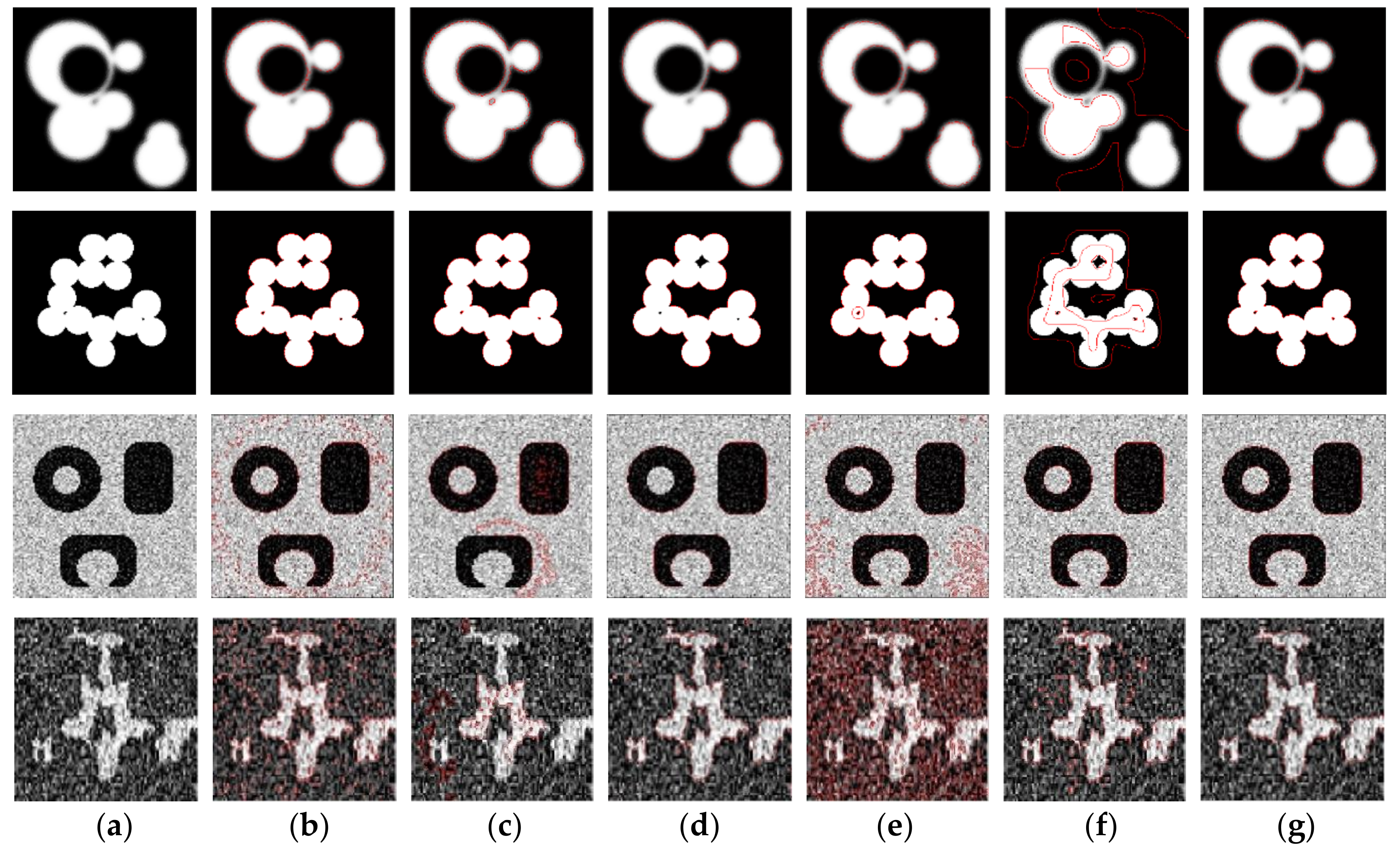
This portion of our experiment concerns the segmentation results obtained for multiobjective images. The SPFLIF-IS method is consistently compared with the five abovementioned methods (C–V, LBF, SBGFRLS, LIF, and LSACM). The original multiobjective images and the segmentation results of the six models are shown in Figure 3, where the original images shown in Figure 3a are derived from [42,49]. Although our model identifies most of the boundaries of the first image, the boundaries are subtle different when compared with those detected by the LBF model. As shown in Figure 3d,f, the SBGFRLS model and the LSACM model obviously fail to segment the first, second, and fourth multiobjective images. The true boundaries of the third image cannot be extracted by the C–V model, the LBF model, the SBGFRLS model, or the LIF model; the results are shown in Row 3 of Figure 3.

Table 2. Description of the segmentation results of Figure 3.

Methods	C–V	LBF	SBGFRLS	LIF	LSACM	SPFLIF-IS
Segmentation performance	F2	T	F3	F2	F1	F2
	T	F2	F3	F1	F1	T
	F1	F1	F3	F1	T	T
	F1	F1	F1	F1	F1	T

describes the segmentation results shown in Figure 3. As shown in Table 2, the SPFLIF-IS yields the best results, the C–V performs as well as the LBF, and the LIF exhibits the worst results. Figure 3 and Table 2 clearly show that our proposed SPFLIF-IS method can segment the fourth image, but the other comparison methods cannot. The experimental results indicate that the SPFLIF-IS model can efficiently segment the multiobjective images.

4.4. Segmentation Results of Noisy Images

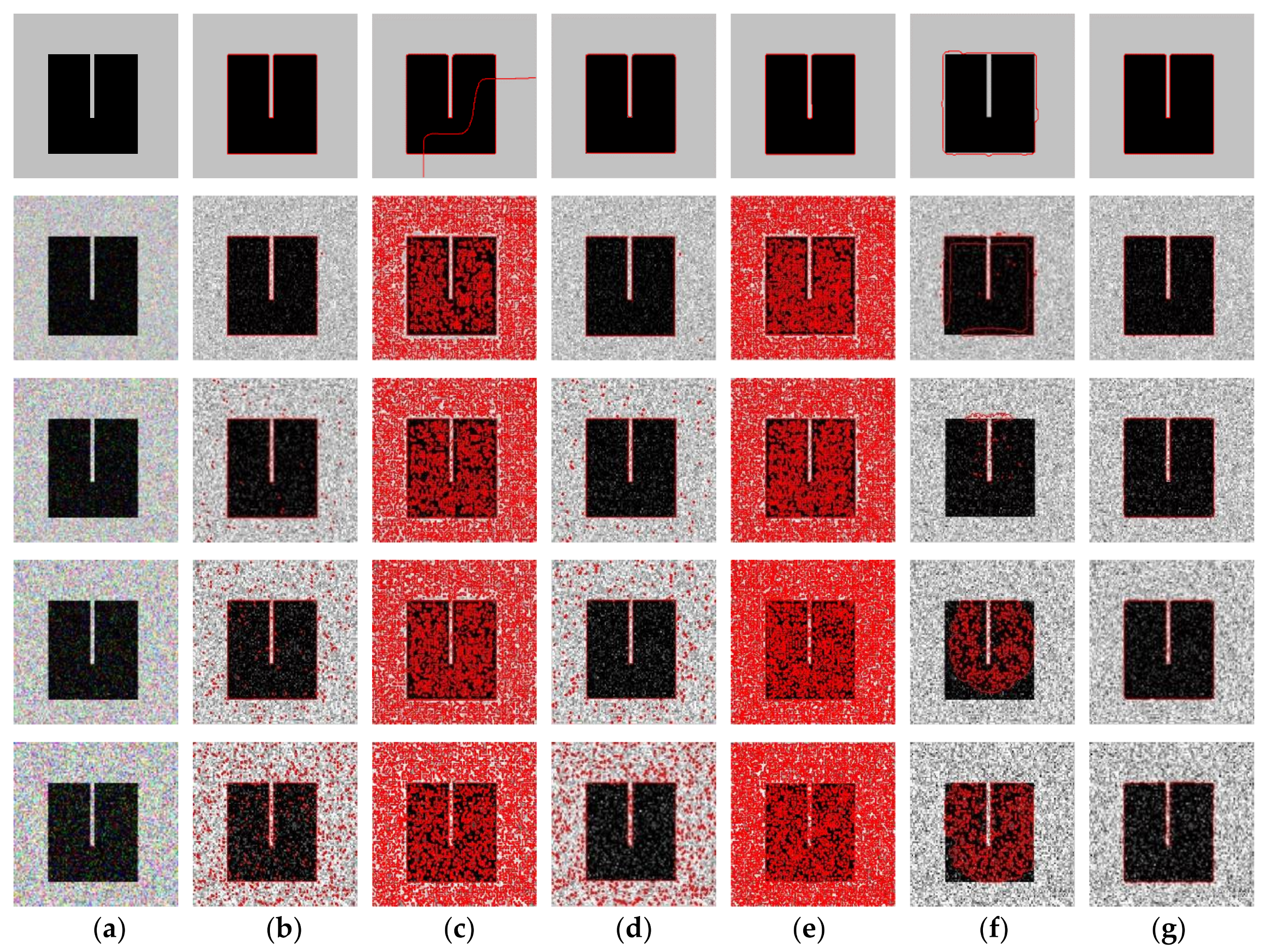
The following subsection describes the experimental segmentation results obtained for noisy images. The SPFLIF-IS model is still compared with the C–V, LBF, SBGFRLS, LIF, and LSACM models. Figure 4 illustrates the original images with different noise intensities and compares the results of the six state-of-the-art segmentation methods, where the original images without noise in Figure 4a are derived from [46]. In Figure 4, Row 1 shows the original images and the segmentation results. Row 2 to Row 5 show the added Gaussian noise with zero means and different variances (σ = 0.01, 0.02, 0.03, 0.05). Figure 4c,f shows that the LBF model and the LSACM model cannot analyze the five images. Although the C–V model and the SBGFRLS model can segment the first and the second image, neither model performs well when the noise intensity increases; the results are shown in Figure 4b,d. Figure 4e shows that the LIF model could analyze the images without Gaussian noise well. With respect to the segmentation of the images containing Gaussian noise, the LIF model exhibits poor performance. As shown in Figure 4g, the object boundaries are accurately extracted by our proposed SPFLIF-IS model.

Table 3. Description of the segmentation results of Figure 4.

Methods	C–V	LBF	SBGFRLS	LIF	LSACM	SPFLIF-IS
Segmentation performance	T	F1	T	T	F1	T
	F2	F1	F2	F1	F1	T
	F1	F1	F1	F1	F1	T
	F1	F1	F1	F1	F1	F2
	F1	F1	F1	F1	F1	F2

describes the segmentation results of Figure 4. Table 3 shows that the SPFLIF-IS model yields the best results, the C–V model performs as well as the SBGFRLS model, and the LBF model performs as poorly as the LSACM model. The experimental results demonstrate that the SPFLIF-IS model can effectively eliminate the interference of the noise and complete the segmentation of the noisy images.

4.5. Segmentation Results of Texture Image

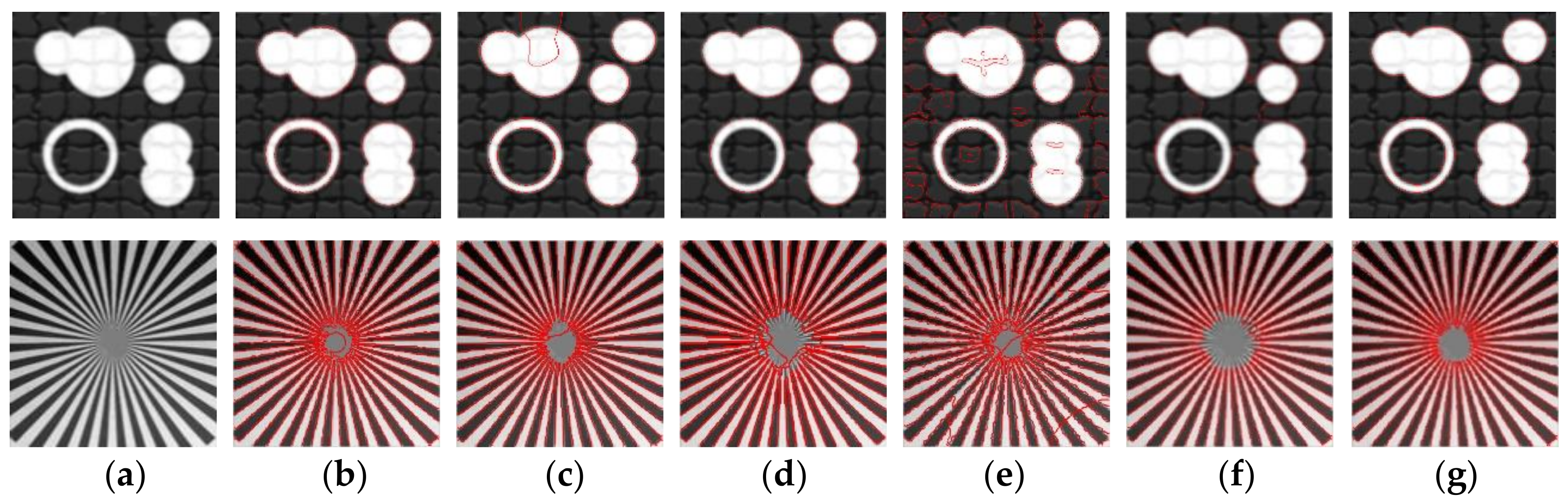
This part of our experiment tests the segmentation performance of texture images. Figure 5a shows the original texture image, which is derived from [4]. Moreover, the compared models are still the C–V, LBF, SBGFRLS, LIF, and LSACM models. According to Figure 5c,e,f, the object boundaries of the first image are not identified by the LBF, LIF, or LSACM model, respectively. Most of the boundaries are obtained by the SBGFRLS model. However, the internal details are not recognized; the detailed results are illustrated in Figure 5d. Figure 5e shows that the LIF model fails to segment the second image. Although the C–V, LBF, SBGFRLS, and LSACM models recognize the true boundaries of the second image, some boundaries lie in the middle of the image; the results are illustrated in Row 2 of Figure 5.

Table 4. Description of the segmentation results of Figure 5.

Methods	C–V	LBF	SBGFRLS	LIF	LSACM	SPFLIF-IS
Segmentation performance	T	F1	F3	F1	F1	T
	F3	F3	F3	F1	F1	T

describes the segmentation results of Figure 5. Table 4 shows that the SPFLIF-IS model performs the best, the C–V model exhibits the second best performance, and the LIF model shows as poor a performance as the LSACM model. The SPFLIF-IS model can eliminate the interference of the image texture and analyze the texture image well.

4.6. Segmentation Results of Real Images

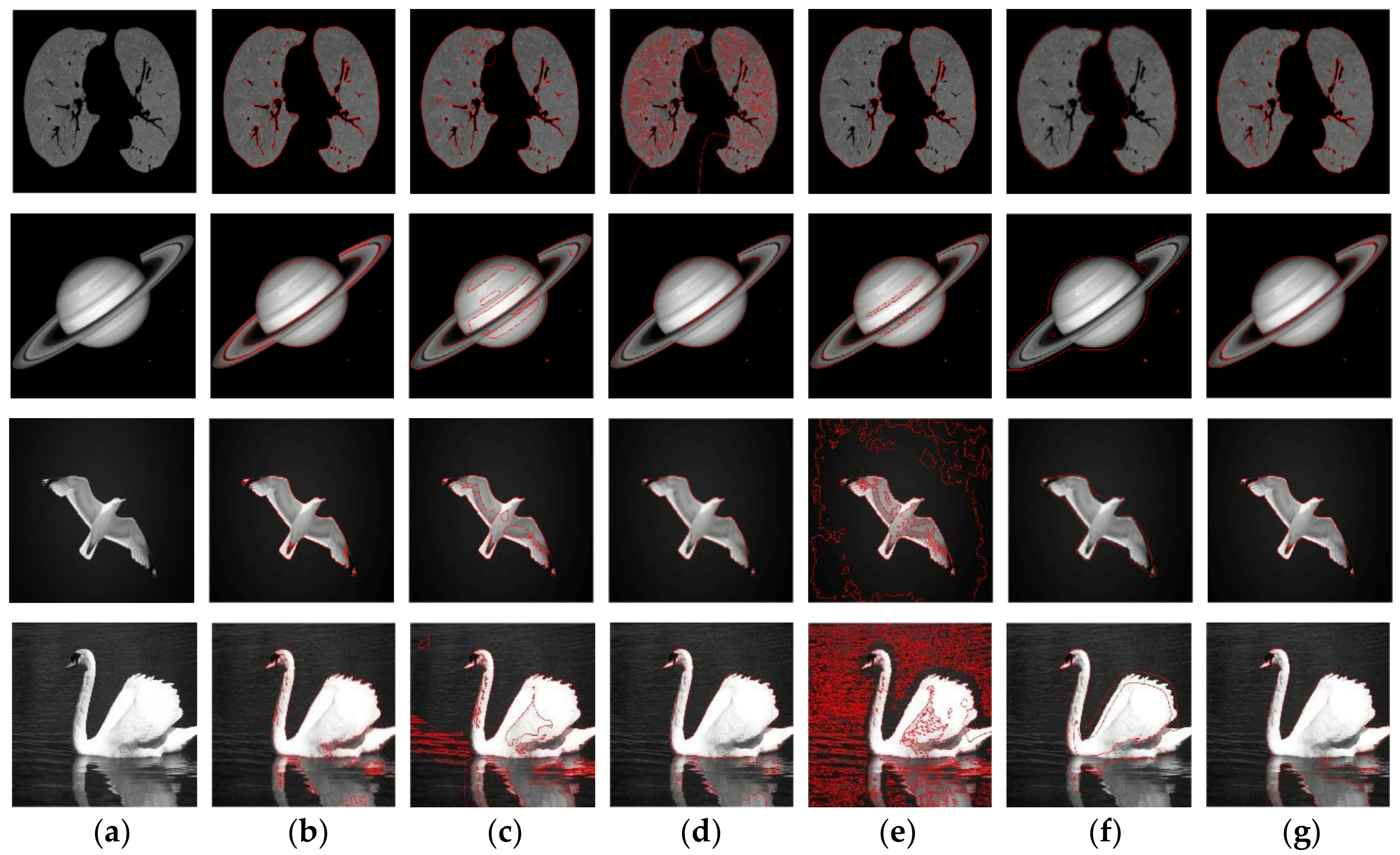
In this subsection, we continue testing our algorithms, this time using real images. The SPFLIF-IS method is compared with the same five methods (C–V, LBF, SBGFRLS, LIF, and LSACM). The original real images and the segmentation results of the six models are shown in Figure 6, where the first and second images in Figure 6a can be found in the literature [27,31], and the third and fourth images shown in Figure 6a are selected from Berkeley segmentation data set 500 (BSDS500) (The code is available at [50]). The first image in the third and fourth columns shows that the LBF and SBGFRLS models fail to segment the image; the results are shown in Figure 6c,d. The first image in the fifth and sixth columns shows that most of the boundaries are obtained by the LIF and LSACM models. However, the internal details are not recognized; the results are illustrated in Figure 6e,f. The LBF, LIF, and LSACM models fail to segment the second and third images, as shown in Figure 6c,e,f. The object boundaries of the fourth images are not accurately extracted by the C–V, LBF, SBGFRLS, LIF, and LSACM models, as shown in the fourth rows of Figure 6. As shown in Figure 6g, the object boundaries are accurately extracted by our proposed model.

Table 5. Description of the segmentation results of Figure 6.

Methods	C–V	LBF	SBGFRLS	LIF	LSACM	SPFLIF-IS
Segmentation performance	T	F1	F1	F3	F1	T
	F2	F1	F2	F1	F1	T
	T	F1	F2	F1	F1	T
	F1	F1	F2	F1	F1	T

objectively offers the segmentation results of Figure 6. Table 5 indicates that the SPFLIF-IS achieves the best results; the C–V exhibits slightly better results than those obtained by the LBF, SBGFRLS, LIF, and LSACM; and the LBF performs as poorly as the LSACM. The segmentation results demonstrate that our SPFLIF-IS model can efficiently analyze real images and yield great segmentation results.

4.7. Comparative Evaluation Results

In addition to using visual evaluation, the accuracy of the target region segmentation can be assessed quantitatively and objectively using the DICE coefficient (DICE) [51,52] and the Jaccard similarity index (JSI) [53]. Following the experimental techniques designed in [42,54], test images are selected randomly from the BSDS500 database. Note that BSDS500 contains hundreds of natural images whose ground-truth segmentation maps have been generated by multiple individuals [40,55]. To enhance the coherency of our work with the abovementioned algorithms, three comparative experiments are performed on many real-world color images, which are selected from the Berkeley segmentation data set 500 (BSDS500) and consist of a set of natural images.

The first part of this experiment involves evaluating the value of the DICE for twenty representative real-world color images, which are chosen from the Berkeley segmentation data set 500 (BSDS500). The algorithms compared are the C–V model [34], the LBF model [24], and the LIF model [31].

The DICE, also called the overlap index, is the most frequently used metric for validating image segmentations. The DICE measures how well the segmentation results S match the ground truth G. When the value of the DICE is close to 1, the segmentation results have high accuracy. The formula for the DICE is given as

$$DICE(G,S)=\frac{2|{\mathsf{\Omega }}_G\cap {\mathsf{\Omega }}_S|}{|{\mathsf{\Omega }}_G|+|{\mathsf{\Omega }}_S|},$$

(25)

where Ω_S describes the segmented volume and Ω_G denotes the ground truth [56,57]. The DICE values of the segmentation results obtained by applying the four models to segment Berkeley color images are listed in

Table 6. DICE values of the image segmentation results using the four models for Berkeley color images.

Image ID	C–V	LBF	LIF	SPFLIF-IS
3063	0.9779	0.9576	0.8962	0.9783
8068	0.978	0.9555	0.8673	0.9827
14092	0.9235	0.871	0.8058	0.9257
29030	0.9525	0.9432	0.8106	0.9743
41004	0.9763	0.9565	0.8769	0.9791
41006	0.9625	0.9305	0.8358	0.9643
46076	0.9763	0.9512	0.8392	0.9783
48017	0.9526	0.9066	0.855	0.9562
49024	0.9566	0.9627	0.8531	0.9792
51084	0.9253	0.9401	0.8464	0.9607
62096	0.9641	0.9387	0.8617	0.9734
101084	0.8942	0.8441	0.8103	0.978
124084	0.9578	0.9378	0.8865	0.9616
143090	0.9575	0.9517	0.8633	0.9692
147091	0.9693	0.9387	0.8254	0.9717
207056	0.9677	0.9305	0.8183	0.9826
296059	0.947	0.9276	0.8283	0.9742
299091	0.9708	0.9595	0.8448	0.9759
317080	0.9591	0.9288	0.8665	0.9634
388006	0.9676	0.9452	0.8738	0.9701
Mean	0.9568	0.9339	0.8483	0.9699

, where the Mean describes the average values of the DICE for all test image data. Table 6 shows that the SPFLIF-IS method yields the best values for the DICE on the twenty image data, and the corresponding Mean is also the largest. The results indicate that our SPFLIF-IS model outperforms the C–V, LBF, and LIF models. In summary, these results demonstrate that our SPFLIF-IS method is indeed efficient and outperforms these currently available approaches.

The next section of the experiment involves testing the value of the JSI coefficient for the twenty representative real-world color images in Table 6. The algorithms compared are still the C–V model [34], the LBF model [24], and the LIF model [31].

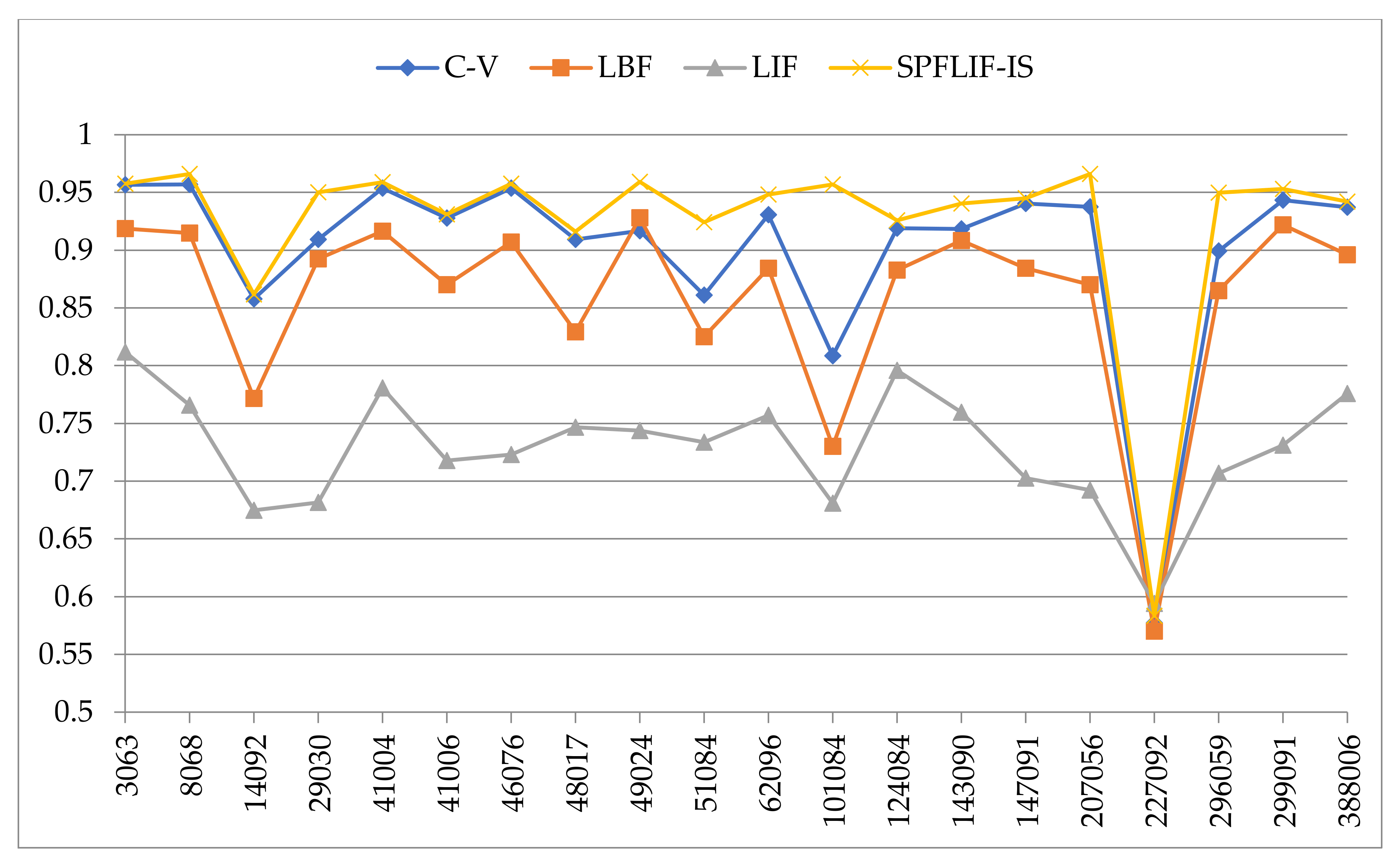
The JSI is the second statistical measure used for quantitative evaluation in this paper. The JSI is calculated by

$$JSI(G,S)=\frac{|{\mathsf{\Omega }}_G\cap {\mathsf{\Omega }}_S|}{|{\mathsf{\Omega }}_G\cup {\mathsf{\Omega }}_S|}.$$

(26)

The accuracy of the segmentation results for the Berkeley color images is measured by the JSI value, as shown in Figure 7. A JSI value close to 1 indicates favorable segmentation results. Figure 7 shows that the SPFLIF-IS method exhibits the best JSI values for the twenty image data. For image IDs 3063, 14092, 41006, and 147091, the JSI values of the C–V model are very close to those of the SPFLIF-IS model. For image ID 227092, the JSI values yielded by the C–V and LBF models are close to those of the SPFLIF-IS model. However, Figure 7 clearly illustrates that the SPFLIF-IS method yields greater JSI values than those generated by the C–V, LBF, and LIF models.

In the final part of this experiment, to fully validate the advantages of our SPFLIF-IS method in terms of the DICE and JSI, the five state-of-the-art methods ((1) the C–V model [34], (2) the LBF model [24], (3) the LIF model [31], (4) the SBGFRLS model [23], and (5) the LSACM model [28]) are applied to eight real color image data selected from the Berkeley segmentation data set 500 (BSDS500). The experimental results are shown in

Table 7. DICE and JSI values of the results of image segmentation on fifteen Berkeley color images.

Image ID	C–V		LBF		SBGFRLS		LIF		LSACM		SPFLIF-IS
	DICE	JSI	DICE	JSI	DICE	JSI	DICE	JSI	DICE	JSI	DICE	JSI
3063	0.9779	0.9568	0.9576	0.9186	0.9728	0.9470	0.8962	0.8119	0.9774	0.9557	0.9783	0.9575
8068	0.9780	0.9570	0.9555	0.9149	0.9785	0.9579	0.8673	0.7657	0.9710	0.9436	0.9827	0.9660
29030	0.9525	0.9093	0.9432	0.8925	0.9709	0.9435	0.8106	0.6815	0.9626	0.9280	0.9743	0.9500
41004	0.9763	0.9537	0.9565	0.9166	0.9775	0.9560	0.8769	0.7808	0.9741	0.9494	0.9791	0.9590
46076	0.9763	0.9537	0.9512	0.9070	0.9753	0.9518	0.8392	0.7230	0.9692	0.9402	0.9783	0.9575
207056	0.9677	0.9375	0.9305	0.8700	0.9774	0.9558	0.8183	0.6924	0.9785	0.9579	0.9826	0.9659
296059	0.9470	0.8994	0.9276	0.8650	0.9684	0.9387	0.8283	0.7069	0.9741	0.9495	0.9742	0.9498
299091	0.9708	0.9433	0.9595	0.9221	0.9750	0.9512	0.8448	0.7313	0.9694	0.9406	0.9759	0.9530
Mean	0.9683	0.9388	0.9477	0.9008	0.9745	0.9502	0.8477	0.7367	0.9720	0.9456	0.9782	0.9573

, where the Mean describes the average values of the DICE and JSI for all test image data.

The foregoing experimental analysis demonstrates that our proposed method is designed based on an improved SPF function and the LIF method. The model combines the merits of global image information and local image information and can segment noisy images and multiobjective images well. By contrast, the C–V model and the SBGFRLS model are constructed with global image information alone, based on the assumption that the region to be segmented is homogeneous. Unfortunately, this assumption is not suitable for intensity-inhomogeneous images [2,31,35]. The LBF model and LIF model use local information to segment intensity-inhomogeneous images and obtain desirable segmentation results; thus, the models are sensitive to the initial position and image noise [2,36]. The LSACM model is proposed based on the local statistical information of an image; therefore, this model is robust to noise while suppressing intensity overlap to some extent. Nevertheless, this model is assumed that the image gray is separable in a relatively small area, and the offset is smooth in the entire image area. The model is easily trapped in a local minimum and involves high computational complexity [58,59]. It follows from Table 7 that the values of the DICE and JSI of the SPFLIF-IS method are the highest for the eight real image data, and the Mean is also the largest. Thus, the experimental results obtained for synthetic and real images further demonstrate the superior performance of our method. Therefore, our model is able to obtain better DICE and JSI values than those yielded by the methods compared.

4.8. Discussion

According to the experimental results and evaluations presented above, the validity and stability of our proposed model are fully verified, and the contributions of the proposed model can be summarized as follows.

(1) The new model is regularized by a Gaussian kernel, which avoids the expensive computation associated with reinitialization. It follows that the model has low computational complexity.

(2) Our proposed model makes the best use of global and local image information. The model solves the problem of not accurately segmenting intensity-inhomogeneous images faced by the traditional image segmentation model and overcomes the shortcoming that local image information is sensitive to the initial contour and noise.

(3) Compared with the existing C–V, LBF, SBGFRLS, LIF, and LSACM models, the SPFLIF-IS model exhibits high robustness to the initial contour and noise and quickly and accurately segments inhomogeneous and multiobjective images.

5. Conclusions

In this paper, to segment intensity-inhomogeneous images quickly and accurately, an image segmentation method using a novel ACM based on an improved SPF function and an LIF model is proposed. The model combines the advantages of global and local information terms in segmenting intensity-inhomogeneous images. Moreover, a weight function is established to adjust the weights between the local information term and the global information term. Thus, a novel ACM model is presented, and an image segmentation algorithm is thereby established. To demonstrate the effectiveness of our proposed model, several experiments are designed in our study. The results indicate that our model not only segments inhomogeneous and multiobjective images effectively but also exhibits high robustness to the initial contour and noise. However, at present, it is difficult to determine a suitable Gaussian kernel size for all the images, and considering the uncertainty of real-world complex images, the proposed method will not be suitable in all the cases. As future work, we plan to accommodate the Gaussian kernel size automatically, which can be used to control region scalability from a small neighborhood to the entire image domain. This approach is considered to be more accurate and efficient in segmenting complex images and reducing computational complexity.

References

- Mabood, L.; Ali, H.; Badshah, N.; Chen, K.; Khan, G.A. Active contours textural and inhomogeneous object extraction. Pattern Recognit. 2016, 55, 87–99. [Google Scholar] [CrossRef]
- Zhao, L.K.; Zheng, S.Y.; Wei, H.T.; Gui, L. Adaptive active contour model driven by global and local intensity fitting energy for image segmentation. Opt. Int. J. Light Electron Opt. 2017, 140, 908–920. [Google Scholar] [CrossRef]
- Kass, M.; Witki, A.; Terzopoulos, D. Snakes: Active contour models. Int. J. Comput. Vis. 1988, 1, 321–331. [Google Scholar] [CrossRef] [Green Version]
- Hai, M.; Jia, W.; Wang, X.F.; Zhao, Y.; Hu, R.X.; Luo, Y.T.; Xue, F.; Lu, J.T. An intensity-texture model based level set method for image segmentation. Pattern Recognit. 2015, 48, 1547–1562. [Google Scholar]
- Wang, X.F.; Huang, D.S.; Xu, H. An efficient local Chan-Vese model for image segmentation. Pattern Recognit. 2010, 43, 603–618. [Google Scholar] [CrossRef]
- Gao, S.; Bui, T.D. Image segmentation and selective smoothing by using Mumford-Shah model. IEEE Trans. Image Process. 2005, 14, 1537–1549. [Google Scholar]
- Hao, R.; Qiang, Y.; Yan, X.F. Juxta-Vascular pulmonary nodule segmentation in PET-CT imaging based on an LBF active contour model with information entropy and joint vector. Comput. Math. Methods Med. 2018, 2018, 2183847. [Google Scholar] [CrossRef] [PubMed]
- Xie, X.H.; Mirmehdi, M. MAC: Magnetostatic active contour model. IEEE Trans. Pattern Anal. Mach. Intell. 2008, 30, 632–646. [Google Scholar] [CrossRef] [PubMed]
- Ko, M.; Kim, S.; Kim, M.; Kim, K. A novel approach for outdoor fall detection using multidimensional features from a single camera. Appl. Sci. 2018, 8, 984. [Google Scholar] [CrossRef]
- Jing, Y.; An, J.B.; Liu, Z.X. A novel edge detection algorithm based on global minimization active contour model for oil slick infrared aerial image. IEEE Trans. Geosci. Remote Sens. 2011, 49, 2005–2013. [Google Scholar] [CrossRef]
- Chan, T.F.; Vese, L.A. Active contours without edges. IEEE Trans. Image Process. 2001, 10, 266–277. [Google Scholar] [CrossRef] [PubMed] [Green Version]
- Li, C.M.; Kao, C.Y.; Gore, J.C.; Ding, Z.H. Minimization of region-scalable fitting energy for image segmentation. IEEE Trans. Image Process. 2008, 17, 1940–1949. [Google Scholar]
- Han, B.; Wu, Y.Q. A novel active contour model based on modified symmetric cross entropy for remote sensing river image segmentation. Pattern Recognit. 2017, 67, 396–409. [Google Scholar] [CrossRef]
- Li, C.M.; Huang, R.; Ding, Z.H.; Gatenby, J.C.; Metaxas, D.N.; Gore, J.C. A level set method for image segmentation in the presence of intensity inhomogeneities with application to MRI. IEEE Trans. Image Process. 2011, 20, 2007–2016. [Google Scholar] [PubMed]
- Caselles, V.; Kimmel, R.; Sapiro, G. Geodesic active contours. Int. J. Comput. Vis. 1997, 22, 61–79. [Google Scholar] [CrossRef]
- Song, Y.; Wu, Y.Q.; Dai, Y.M. A new active contour remote sensing river image segmentation algorithm inspired from the cross entropy. Digit. Signal Process. 2016, 48, 322–332. [Google Scholar] [CrossRef]
- Cao, G.; Mao, Z.H.; Yang, X.; Xia, D.S. Optical aerial image partitioning using level sets based on modified Chan-Vese model. Pattern Recognit. Lett. 2008, 29, 457–464. [Google Scholar] [CrossRef]
- Li, X.M.; Jiang, D.S.; Shi, Y.H.; Li, W.S. Segmentation of MR image using local and global region based geodesic model. Biomed. Eng. Online 2015, 14, 8. [Google Scholar] [CrossRef] [Green Version]
- Liu, S.G.; Peng, Y.L. A local region-based Chan–Vese model for image segmentation. Pattern Recognit. 2012, 45, 2769–2779. [Google Scholar] [CrossRef]
- Wang, L.; He, L.; Mishra, A.; Li, C.M. Active contours driven by local Gaussian distribution fitting energy. Signal Process. 2009, 89, 2435–2447. [Google Scholar] [CrossRef]
- Zhang, L.; Peng, X.G.; Li, G.; Li, H.F. A novel active contour model for image segmentation using local and global region-based information. Mach. Vis. Appl. 2017, 28, 75–89. [Google Scholar] [CrossRef]
- Soomro, S.; Akram, F.; Munir, A.; Lee, C.H.; Choi, K.N. Segmentation of left and right ventricles in cardiac MRI using active contours. Comput. Math. Methods Med. 2017, 2017, 1455006. [Google Scholar] [CrossRef] [PubMed]
- Zhang, K.H.; Zhang, L.; Song, H.H.; Zhou, W.G. Active contours with selective local or global segmentation: A new formulation and level set method. Image Vis. Comput. 2010, 28, 668–676. [Google Scholar] [CrossRef]
- Li, C.M.; Kao, C.Y.; Gor, J.C.; Ding, Z.H. Implicit active contours driven by local binary fitting energy. In Proceedings of the IEEE Conference on Computer Vision & Pattern Recognition, Minneapolis, MN, USA, 17–22 June 2007; pp. 1–7. [Google Scholar]
- Yuan, J.J.; Wang, J.J. Active contours driven by local intensity and local gradient fitting energies. Int. J. Pattern Recognit. Artif. Intell. 2014, 28, 1455006. [Google Scholar] [CrossRef]
- Tu, S.; Su, Y. Fast and accurate target detection based on multiscale saliency and active contour model for high-resolution SAR images. IEEE Trans. Geosci. Remote Sens. 2016, 54, 5729–5744. [Google Scholar] [CrossRef]
- Wang, L.; Li, C.M.; Sun, Q.S.; Xia, D.S.; Kao, C.Y. Active contours driven by local and global intensity fitting energy with application to brain MR image segmentation. Comput. Med Imaging Graph. 2009, 33, 520–531. [Google Scholar] [CrossRef] [PubMed]
- Zhang, K.H.; Zhang, L.; Lam, K.M.; Zhang, D. A level set approach to image segmentation with intensity inhomogeneity. IEEE Trans. Cybern. 2016, 46, 546–557. [Google Scholar] [CrossRef]
- Jiang, X.L.; Li, B.L.; Wang, Q.; Chen, P. A novel active contour model driven by local and global intensity fitting energies. Opt. Int. J. Light Electron Opt. 2014, 125, 6445–6449. [Google Scholar] [CrossRef]
- Zhao, Y.Q.; Wang, X.F.; Shih, F.Y.; Yu, G. A level-set method based on global and local regions for image segmentation. Int. J. Pattern Recognit. Artif. Intell. 2012, 26, 1255004. [Google Scholar] [CrossRef]
- Zhang, K.H.; Song, H.H.; Zhang, L. Active contours driven by local image fitting energy. Pattern Recognit. 2010, 43, 1199–1206. [Google Scholar] [CrossRef]
- Akram, F.; Garcia, M.A.; Puig, D. Active contours driven by local and global fitted image models for image segmentation robust to intensity inhomogeneity. PLoS ONE 2017, 12, e0174813. [Google Scholar] [CrossRef]
- Zhu, H.Q.; Xie, Q.Y. A multiphase level set formulation for image segmentation using a MRF-based nonsymmetric Student’s-t mixture model. Signal Image Video Process. 2018, 18, 1577–1585. [Google Scholar] [CrossRef]
- Wang, X.F.; Min, H.; Zou, L.; Zhang, Y.G. A novel level set method for image segmentation by incorporating local statistical analysis and global similarity measurement. Pattern Recognit. 2015, 48, 189–204. [Google Scholar] [CrossRef]
- Cao, J.F.; Wu, X.J. A novel level set method for image segmentation by combining local and global information. J. Mod. Opt. 2017, 64, 2399–2412. [Google Scholar] [CrossRef]
- Tian, Y.; Duan, F.Q.; Zhou, M.Q.; Wu, Z.K. Active contour model combining region and edge information. Mach. Vis. Appl. 2013, 24, 47–61. [Google Scholar] [CrossRef]
- Lok, K.H.; Shi, L.; Zhu, X.L.; Wang, D.F. Fast and robust brain tumor segmentation using level set method with multiple image information. J. X-ray Sci. Technol. 2017, 25, 301–312. [Google Scholar] [CrossRef]
- Sun, Z.; Qi, M.; Lian, J.; Jia, W.K.; Zou, W.; He, Y.L.; Liu, H.; Zheng, Y.J. Image segmentation by searching for image feature density peaks. Appl. Sci. 2018, 8, 969. [Google Scholar] [CrossRef]
- Xu, H.Y.; Jiang, G.Y.; Yu, M.; Luo, T. A global and local active contour model based on dual algorithm for image segmentation. Comput. Math. Appl. 2017, 74, 1471–1488. [Google Scholar] [CrossRef]
- Abdelsamea, M.M. A semi-automated system based on level sets and invariant spatial interrelation shape features for Caenorhabditis elegans phenotypes. J. Vis. Commun. Image Represent. 2016, 41, 314–323. [Google Scholar] [CrossRef]
- Ji, Z.X.; Xia, Y.; Sun, Q.S.; Gao, G.; Chen, Q. Active contours driven by local likelihood image fitting energy for image segmentation. Inf. Sci. 2015, 301, 285–304. [Google Scholar] [CrossRef]
- Xu, C.Y.; Yezzi, A.; Prince, J.L. On the relationship between parametric and geometric active contours. In Proceedings of the IEEE Conference Record of the 34th Asilomar Conference on Signals, Systems and Computers, Pacific Grove, CA, USA, 29 October–1 November 2000; pp. 483–489. [Google Scholar]
- Abdelsamea, M.M.; Tsaftaris, S.A. Active contour model driven by globally signed region pressure force. In Proceedings of the IEEE 18th International Conference on Digital Signal Processing, Santorini, Greece, 1–3 July 2013; pp. 1–6. [Google Scholar]
- Li, D.Y.; Li, W.F.; Liao, Q.M. Active contours driven by local and global probability distributions. J. Vis. Commun. Image Represent. 2013, 24, 522–533. [Google Scholar] [CrossRef]
- Hanbay, K.; Talu, M.F. A novel active contour model for medical images via the Hessian matrix and eigenvalues. Comput. Math. Appl. 2018, 75, 3081–3104. [Google Scholar] [CrossRef]
- Vese, L.A.; Chan, T.F. A multiphase level set framework for image segmentation using the Mumford and Shah model. Int. J. Comput. Vis. 2002, 50, 271–293. [Google Scholar] [CrossRef]
- Lei Zhang’s Homepage. Available online: http://www4.comp.polyu.edu.hk/~cslzhang/ (accessed on 10 December 2018).
- Chunming Li’s Homepage. Available online: http://www.engr.uconn.edu/~cmli/ (accessed on 10 December 2018).
- Li, M.; He, C.J.; Zhan, Y. Adaptive regularized level set method for weak boundary object segmentation. Math. Probl. Eng. 2012, 2012, 369472. [Google Scholar] [CrossRef]
- The Berkeley Segmentation Dataset and Benchmark. Available online: https://www2.eecs.berkeley. edu/Research/Projects/CS/vision/bsds/ (accessed on 10 December 2018).
- Jiang, X.L.; Wang, Q.; He, B.; Chen, S.J.; Li, B.L. Robust level set image segmentation algorithm using local correntropy-based fuzzy c-means clustering with spatial constraints. Neurocomputing 2016, 27, 22–35. [Google Scholar] [CrossRef]
- Dice, L.R. Measures of the amount of ecologic association between species. Ecology 1945, 26, 297–302. [Google Scholar] [CrossRef]
- Jaccard, P. The distribution of the flora in the alpine zone. New Phytol. 1912, 11, 37–50. [Google Scholar] [CrossRef]
- Wang, L.; Chang, Y.; Wang, H.; Wang, Z.Z.; Pu, J.T.; Yang, X.D. An active contour model based on local fitted images for image segmentation. Inf. Sci. 2017, 418, 61–73. [Google Scholar] [CrossRef] [Green Version]
- Arbelaez, P.; Maire, M.; Fowlkes, C.; Malik, J. Contour detection and hierarchical image segmentation. IEEE Trans. Pattern Anal. Mach. Intell. 2011, 33, 898–916. [Google Scholar] [CrossRef]
- Zhao, W.; Fu, Y.; Wei, X.; Wang, H. An improved image semantic segmentation method based on superpixels and conditional random fields. Appl. Sci. 2018, 8, 837. [Google Scholar] [CrossRef]
- Zhou, S.P.; Wang, J.J.; Zhang, M.M.; Cai, Q.; Gong, Y.H. Correntropy-based level set method for medical image segmentation and bias correction. Neurocomputing 2017, 234, 216–229. [Google Scholar] [CrossRef]
- Zhang, Y.C. Research of level set image segmentation based on Rough Set theory and the extended watershed transformation. Ph.D. Thesis, Dalian University of Technology, Dalian, China, 2018; pp. 4–6. [Google Scholar]
- Sun, L.; Meng, X.C.; Xu, J.C.; Zhang, S.G. An image segmentation method based on improved regularized level set model. Appl. Sci. 2018, 8, 2393. [Google Scholar] [CrossRef]
Figure 1.
The graphical process of image segmentation.
Figure 2.
The segmentation results of images with intensity inhomogeneity for the six models. (a) Original image, (b) C–V model, (c) LBF model, (d) SBGFRLS model, (e) LIF model, (f) LSACM model, and (g) SPFLIF-IS model.
Figure 3.
The segmentation results of the multiobjective images for the six models. (a) Original image, (b) C–V model, (c) LBF model, (d) SBGFRLS model, (e) LIF model, (f) LSACM model, and (g) SPFLIF-IS model.
Figure 4.
The segmentation results obtained for images with strong noise using the six models. (a) Original image, (b) C–V model, (c) LBF model, (d) SBGFRLS model, (e) LIF model, (f) LSACM model, and (g) SPFLIF-IS model.
Figure 5.
The segmentation results obtained for a texture image using the six models. (a) Original image, (b) C–V model, (c) LBF model, (d) SBGFRLS model, (e) LIF model, (f) LSACM model, and (g) SPFLIF-IS model.
Figure 6.
The segmentation results obtained for real images using the six models. (a) Original image, (b) C–V model, (c) LBF model, (d) SBGFRLS model, (e) LIF model, (f) LSACM model, and (g) SPFLIF-IS model.
Figure 7.
JSI values of the image segmentation results using the four models for Berkeley color images.