Factorial Design Analysis for Localization Algorithms

Abstract

Localization is a fundamental problem in Wireless Sensor Networks, as it provides useful information regarding the detection of an event. There are different localization algorithms applied in single-hop or multi-hop networks; in both cases their performance depends on several factors involved in the evaluation scenario such as node density, the number of reference nodes and the log-normal shadowing propagation model, determined by the path-loss exponent ($\eta$) and the noise level (${\sigma }_{dB}$) which impact on the accuracy and precision performance metrics of localization techniques. In this paper, we present a statistical analysis based on the $2^k$ factorial methodology to determine the key factors affecting the performance metrics of localization techniques in a single-hop network to concentrate on such parameters, thus reducing the amount of simulation time required. For this proposal, MATLAB simulations are carried out in different scenarios, i.e., extreme values are used for each of the factors of interest and the impact of the interaction among them in the performance metrics is observed. The simulation results show that the path-loss exponent ($\eta$) and noise level (${\sigma }_{dB}$) factors have the greatest impact on the accuracy and precision metrics evaluated in this study. Based on this statistical analysis, we recommend estimating the propagation model as close to reality as possible to consider it in the design of new localization techniques and thus improve their accuracy and precision metrics.

1. Introduction

Wireless Sensor Networks (WSN) are relevant in the real world because they can determine physical behaviors based on the collaborative work of many sensors [1]. There are several applications for this kind of network, and they can be classified into two categories: monitoring and tracking [2]. There is also a taxonomy of the application domains [3]. The taxonomy includes military and crime prevention [4], disaster prevention and reduction crime in the city [5], health care (Body Area Networks) [6,7,8], industry and agriculture [9,10,11], urbanization [12] and environmental monitoring applications [13,14,15].

The task of collecting data is well defined if the location of sensors is known [16]; localization information is also useful for coverage estimation, deployment, routing, location service, target tracking, and rescue [17,18]. A solution is to add GPS receivers, but it is expensive and inconvenient for some application scenarios, such as indoors. Localization is one of the main problems in WSNs, since location information is essential for the detection of an event. In the field of underwater environments, localization is one of the most important technologies, since it plays a critical role in many applications. Some applications in underwater environments where location is useful are: data collection, climate change, aquatic animal life time and coral reef population variations, underwater exploration, natural disaster prevention (tornadoes, hurricanes, tsunamis, etc.), ecological applications (pollution, water quality, environmental monitoring, etc.), assisted navigation, military surveillance, etc. The localization problem in WSN is addressed with different approaches; nevertheless, the inherent characteristics of a WSN, such as limited processing resources, storage, and power, inevitably make localization an engineering challenge. In that sense, several proposals, including some novel solutions, have been developed; in most cases, the evaluation of proposals is done through simulations since their physical implementation involves a high cost and intensive work. The evaluation of all proposals is based on common metrics related to the estimation error and the cost, (i.e., accuracy, precision, and computational complexity [19,20]). The network’s performance can be influenced by the choice of key factors when a localization scenario is simulated, for example, node density [21], and propagation model, among others, and the simulation of all possible combinations can prove to be excessive.

The main purpose of this paper is to qualitatively determine the key factors affecting the accuracy and precision performance metrics of localization techniques in some of the principal localization algorithms in a single-hop network, to concentrate on such parameters, thus reducing the amount of simulation time required. For this proposal, the $2^k$ factorial design analysis methodology is used, and MATLAB simulations are carried out in different scenarios, i.e., the extremes values are used for each of the factors of interest and the impact of the interaction among them in the performance metrics is observed. It is important to point out that there is a high degree of variability in some of the simulation factors reported in the literature, and up to now no study has been done of the factors’ impact in the performance of localization techniques or on the relations among them. In other words, the literature reports many proposals to improve localization algorithms, but their design is not based on the factors that have the greatest impact on performance metrics; they are only used to evaluate their algorithm. Thus, the main contribution of this paper is to formally identify these factors to generate more precise and accurate localization algorithms.

The remainder of the paper is organized as follows: Section 2 describes the classification of localization techniques and some scenarios for evaluating localization algorithm performance in real and simulated environments [19,22,23,24,25,26]; mention is also made of some examples of experiment designs that use $2^k$ factorial analysis [27,28,29,30]. Section 3 describes the $2^k$ factorial methodology used. Section 4 shows the results of the study factors’ impact on the localization algorithms’ performance metrics. Next, the conclusions of this paper are presented: the main results, the paper’s contribution, and proposed future lines of research. Finally, the references that sustain the validity of this paper are presented.

2. Related Work

2.1. Classification of the Localization Techniques

Localization techniques are classified into two categories: range-free [31] and range-based [19]. The former use connectivity information from the network to estimate the distance between the Node of Interest (NOI) and the Reference Nodes (RNs). This group includes techniques such as centroid; Distance Vector-Hop (DV-Hop) [32]; Approximate Point In Triangle (APIT); circular, rectangular, and hexagonal interaction, respectively; among others. Range-free localization techniques are more inaccurate in localizing the NOI than range-based localization techniques, but they are less complex in terms of computational cost [19]. Range-based techniques, for their part, need distance between the NOI and the RNs to estimate the position of the NOI. The distance between the NOI and the RNs can be calculated using the Received Signal Strength (RSS), Time of Arrival (ToA), Time Difference of Arrival (TDoA) or Angle of Arrival (AoA) [19]. Some range-based localization techniques are multilateration, Multidimensional-Scaling (MDS), hyperbolic and weighted hyperbolic positioning algorithm, circular and weighted circular positioning algorithm, and Weighted Least-Squares (WLS) multilateration [19].

In [19,31] the range-free and range-based localization techniques are evaluated using three performance metrics: Mean Squared Error (MSE), Cumulative Distribution Function (CDF), and computational complexity. Christine L. and Michel B. Ref. [22], as in [23], use the Average Localization Error (ALE) and the CDF to measure the performance of free-range localization techniques and [23] also uses them in range-based techniques.

In multi-hop scenarios the DV-Hop, Improved DV-Hop (IDV-Hop) and Weighted DV-Hop (WDV-Hop) algorithms are used to estimate the distance between the NOI and the RNs using the number of hops between them [32]. The algorithms DV-Hop and its variations IDV-Hop and WDV-Hop use the network connectivity information to estimate the average distance per hop. Once the average distance per hop is obtained, the distance separating the NOI and the RNs is obtained to estimate the position of the NOI. There are different localization techniques to estimate the position of the NOI. In [33] the Least-Squares DV-Hop (LSDV-Hop) algorithm is used; this improves the accuracy of the localization of the NOI by extracting a minimum-squares transformation vector between the real and estimated position of the RNs, which are chosen at random. This method does not require extra hardware to estimate the position of the NOI, and it is more suitable for networks with high node densities and long scale. In [32] the hyperbolic and weighted hyperbolic algorithm is used to estimate the position of the NOI; the weighted hyperbolic algorithm offers better performance than the hyperbolic algorithm in terms of the accuracy of the position of the NOI, because this method uses a covariance matrix, whose elements from the main diagonal depend on the estimated distance between the NOI and the RNs. In [34] the meta-heuristic optimization algorithm is used based on Particle Swarm Optimization (PSO) to estimate the position of the NOI through an iterative process that minimizes one cost function. In [35] the PSO algorithm is also used with learning strategies; this technique improves convergence speeds and the PSO algorithm’s search efficiency, thus solving the problem of the local minimum of the PSO algorithm. In other multi-hop scenarios, ToA is used to estimate the distance separating the NOI and the RNs [36], where the localization algorithms used are the Vertex-Projection (VP) based on a pyramid-shaped structure; the VP with correction factor, which diminishes the localization error; and the maximum-likelihood algorithm, which shows less localization error than the VP algorithm with the correction factor for high noise levels.

Table 1. Classification of the localization techniques.

Localization Technique	Type	Description	Performance Metrics	Number of Hops	Simulation Environment
CL	range-free	This method calculates the position of the NOI as the centroid of the RNs.	MSE, CDF	One-Hop	Indoors Outdoors
WCL	range-free	Based on the CL algorithm considering a vector of weights, where these weights depend on the distance separating the NOI and the RNs.	MSE, CDF	One-Hop	Indoors Outdoors
RWL	range-free	Based on the WCL algorithm, where the vector of weights depends on a linear relation of the RSS between the NOI and the RNs.	MSE, CDF	One-Hop	Indoors Outdoors
REWL	range-free	Based on the WCL algorithm, where the vector of weights depends on an exponential relation of the RSS between the NOI and the RNs.	MSE, CDF	One-Hop	Indoors Outdoors
DV-Hop	range-free	This method calculates the average distance of a hop on the network, to estimate the distance separating the NOI from the RNs.	MSE, CDF	Multi-Hop	Outdoors
IDV-Hop	range-free	This technique takes the average of all the average distances per hop, to diminish the variance of the average distance per hop.	MSE, CDF	Multi-Hop	Outdoors
WDV-Hop	range-free	This technique considers the average distance per hop calculated by the IDV-Hop algorithm adding a compensation factor.	MSE, CDF	Multi-Hop	Outdoors
PSO	range-free	This localization algorithm calculates the position of the NOI as the overall optimum using an iterative process that minimizes the cost function.	MSE, CDF	Multi-Hop	Outdoors
Hyperbolic	range-based	This method converts the problem of non-linear localization into a linear problem using a least-squares estimator.	MSE, CDF	One-Hop Multi-Hop	Indoors Outdoors
Weighted Hyperbolic	range-based	This method converts the problem of non-linear localization into a linear problem using a weighted least-squares estimator.	MSE, CDF	One-Hop Multi-Hop	Indoors Outdoors
Circular	range-based	This method calculates the position of the NOI by iteratively using the descending gradient method until the cost function is minimized.	MSE, CDF	One-Hop Multi-Hop	Indoors Outdoors
WLS multilateration	range-based	This method converts the problem of non-linear localization into a linear problem using a weighted minimum-squares optimization algorithm.	MSE, CDF	One-Hop Multi-Hop	Indoors Outdoors
Vertex-Projection	range-based	Localization technique of low computational complexity based on a pyramid-shaped structure.	RMSE	One-Hop Multi-Hop	Outdoors
Vertex-Projection Correcting Factor	range-based	Considers a correction factor in the distance separating the NOI from the RNs, which diminishes the localization error.	RMSE	One-Hop Multi-Hop	Outdoors
Maximum-likelihood	range-based	This method uses the maximum-likelihood principle to estimate the distance separating the NOI from the RNs as a function of the number of hops.	RMSE	One-Hop Multi-Hop	Outdoors
LSDV-Hop	range-based	This method improves the precision of the NOI localization by extracting a minimum-squares transformation vector between the real and estimated position of the randomly selected RNs.	ALE	Multi-Hop	Outdoors

shows a classification of the localization techniques according to whether they are distance-based or not, the performance metrics used, the number of hops between the NOI and the RNs, and the simulation environments for which they were designed. Ref. [19] presents the performance evaluation in terms of accuracy and precision measured by the MSE and the CDF, respectively, of range-free localization techniques such as Centroid Localization (CL) [22], Weighted CL (WCL) [22], Relative Weighted Localization (RWL) [22], Relative Exponential Weighted Localization (REWL) [22] and of range-based techniques such as Hyperbolic positioning algorithm, Weighted Hyperbolic positioning algorithm, circular algorithm and WLS multilateration [37], considering a one-hop network and both indoor and outdoor environments. For its part, in [32] performance is also analyzed in terms of accuracy and precision as measured by the MSE and the CDF, respectively, of the localization techniques DV-Hop, IDV-Hop, WDV-Hop, Weighted Hyperbolic positioning algorithm and PSO algorithm [34,35] considering a multi-hop network in an outdoor environment. The performance of the LSDV-Hop algorithm is evaluated in terms of the ALE considering a multi-hop network in outdoor environments [33]. Finally, in [36] the Vertex Projection, Vertex Projection with Correcting Factor and maximum-likelihood algorithms are evaluated for normalized Root Mean Squared Error (RMSE) considering a one-hop and multi-hop network in outdoor environments.

Since the localization techniques described in Table 1 are evaluated in different scenarios and with different performance parameters, they cannot be compared directly. In this paper, four localization techniques were selected, and evaluated in a single localization scenario [19]. In the proposed evaluation scenario, Received Signal Strength Indicator (RSSI) is used to estimate the distance between the NOI and the RNs [19,26].

2.2. Evaluation Scenarios Reported

These localization techniques have been evaluated in different real-world scenarios [23,24,25] and simulations [19,22]. In [24] the authors describe a real-world outdoor scenario with a sensing area measuring 10 m × 10 m and four RNs on the corners of the sensing area, where range-free localization techniques are evaluated [19,22] for their simple implementation in hardware. In this scenario, the log-normal shadowing propagation model is used to calculate the RSSI between the NOI and the four RNs. Since this scenario is represented in a small area, the MSE is evaluated as a function of the noise ${\sigma }_{dB}\in \left\{0.5,1,2,\dots ,10\right\},$ because the number of RNs is always constant and node density is assumed to be unitary, i.e., one NOI on the 10 m × 10 m grid. CDF represents the localization error distribution, when two localization techniques are compared, that technique with a localization error distribution concentrated on the small values is the better [19], since this implies that the technique has a high probability of having small localization errors. Up to now no large sensing area scenario has been used to evaluate localization technique performance. In [23] the authors propose two testbeds for characterizing the channel by means of the RSSI. In this scenario range-free localization algorithms such as Ring Overlapping Circle RSSI (ROCRSSI) [38] and range-based localization algorithms such as minmax [39,40], multilateration [19] and Maximum-Likelihood [36,41] are evaluated in an indoor area measuring 10 m × 10 m with six RNs. These algorithms are evaluated using two testbeds where the ALE is measured by varying the number of RNs and the CDF vs. localization error.

In the simulation scenarios, range-free and range-based localization techniques are evaluated in different sensing areas. In [19] the authors propose a sensing area of 1000 m × 1000 m where the log-normal shadowing propagation model is used. In this scenario the MSE is evaluated based on noise ${\sigma }_{dB}\in \left\{4,\dots ,12\right\}$ dB and node density $\rho \in \left\{1,\dots ,9\right\}$ nodes on an area of 100 m × 100 m. Again, the CDF is evaluated based on localization error. In [22] range-free localization techniques are also evaluated on an area of 1000 m × 1000 m where the log-normal shadowing model is used for different propagation settings, at 2.4 GHz Wi-Fi/802.11g [42,43] and 5.8 GHz [44,45]. In this scenario the localization technique performance is evaluated on the basis of the ALE and the CDF, by varying the node density $\rho \in \left\{0.25,0.5,0.75,1,\dots ,9\right\}$ and the number of RNs $N_{rx}=\left\{2,4,8,16\right\}$ for 2.4 GHz and 5.8 GHz environments.

2.3. Localization Techniques Analyzed

For this paper, four localization techniques were selected to determine the impact of the study factors on the performance metrics of accuracy and precision, using the $2^k$ factorial methodology. The CL and REWL range-free localization techniques were selected, because the CL technique yields the worst performance and the REWL technique yields the best performance in terms of accuracy and precision, respectively, in the proposed evaluation scenario. Range-based localization techniques were also selected, such as the hyperbolic positioning algorithm and the WLS multilateration algorithm, which are the techniques that yield the worst and best performance, respectively, in terms of accuracy and precision in the proposed evaluation scenario. The purpose of selecting range-free and range-based techniques is to determine the localization techniques where the study factors show the greatest impact on their performance in terms of accuracy and precision.

Below are brief descriptions of the selected localization algorithms.

• CL Algorithm

Given a set of $N$ RNs within the range of transmission of the NOI, the localization of the NOI is calculated by way of the average of the positions of the RNs [22]. The centroid p of a set of $N$ RNs is calculated by

$$p=\frac{1}{N}{\displaystyle \sum }_{i=1}^N{p}_i$$

(1)

where $p_i$ is the position with coordinates $\left(x_i,y_i\right)$ of the RN $i$.

• REWL Algorithm

This algorithm is a variation of the WCL algorithm [22]. The weighting factor increases exponentially as the RSS given in dBm increases. Considering a positive real $\lambda$ constant factor between 0 and 1, the weighting factor ${\omega }_i$ of each RN $i$ is given by

$${\omega }_i={\left(1-\lambda \right)}^{v_{max}-v_i}$$

(2)

where $v_i$ is the RSS in dBm between the NOI and the RN $i$ and $v_{max}$ is the maximum RSS of the set of RNs. Therefore, the centroid p of a set of RNs is calculated by

$$p=\frac{{{\displaystyle \sum }}_{i=1}^N{p}_i{\left(1-\lambda \right)}^{v_{max}-v_i}}{{{\displaystyle \sum }}_{i=1}^N{\left(1-\lambda \right)}^{v_{max}-v_i}}.$$

(3)

• Hyperbolic Positioning Algorithm

The hyperbolic positioning algorithm converts the non-linear problem into a linear problem by using a minimum-squares estimator [22]. The distance between a mobile node and the RN $i$ is calculated by the Pythagorean theorem

$$d_i{}^2= {\left(x_i-x\right)}^2+{\left(y_i-y\right)}^2.$$

(4)

Developing the subtraction $d_i{}^2-d_1^2$, Equation (4) becomes a linear problem, leading to the following:

$$2x{x}_i+2y{y}_i-2x{x}_1-2y{y}_1=x_i{}^2+y_i{}^2-x_1{}^2-y_1{}^2-d_i{}^2+d_1{}^2.$$

(5)

Expressing Equation (5) in matrix form for $i=2,\dots ,N$

$$\left[\begin{array}{cc}{x}_2-x_1& y_2-y_1\\ ⋮& ⋮\\ x_N-x_1& y_N-y_1\end{array}\right]\left[\begin{array}{c}x\\ y\end{array}\right]=\frac{1}{2}\left[\begin{array}{c}{x}_2{}^2+y_2{}^2-x_1{}^2-y_1{}^2-d_2{}^2+d_1{}^2\\ ⋮\\ x_N{}^2+y_N{}^2-x_1{}^2-y_1{}^2-d_N{}^2+d_1{}^2\end{array}\right].$$

(6)

Thus, the linear problem can be formulated by

$$Hp=b.$$

(7)

where $H=\left[\begin{array}{cc}{x}_2-x_1& y_2-y_1\\ ⋮& ⋮\\ x_N-x_1& y_N-y_1\end{array}\right],p=\left[\begin{array}{c}x\\ y\end{array}\right]$ and $b$ is a random vector given by

$$b=\frac{1}{2}\left[\begin{array}{c}{x}_2{}^2+y_2{}^2-x_1{}^2-y_1{}^2-d_2{}^2+d_1{}^2\\ ⋮\\ x_N{}^2+y_N{}^2-x_1{}^2-y_1{}^2-d_N{}^2+d_1{}^2\end{array}\right].$$

(8)

Finally, position p of the mobile node can be calculated by the following expression:

$$p={\left(H^{T}H\right)}^{-1}{H}^{T}b$$

(9)

where $p$ is the estimated position of the NOI.

• WLS Multilateration Algorithm

In the presence of unwanted noise, the distance between the RN $i$ and the NOI can be calculated by $r_i=f_i\left(x,y\right)+n_i$, where $f_i\left(x,y\right)$ is the real distance between RN $i$ and the NOI and $n_i$ is a Gaussian random variable, i.e., $n_i~\mathcal{N}\left(0,{\sigma }^2\right)$ [22]. The distance $f_i\left(x,y\right)$ is calculated by the following expression:

$$f_i\left(x,y\right)=\sqrt{{\left(x-x_i\right)}^2+{\left(y-y_i\right)}^2}.$$

(10)

Defining $q={\left[x,y\right]}^H$ as a vector of the position of the NOI, then for a set $N$ observations, the expression $r_i=f_i\left(x,y\right)+n_i$, can be expressed in vector form, i.e., $r=f\left(q\right)+n$. Therefore, the localization problem can be solved by a WLS optimization algorithm as shown in the equation given by

$$\widehat{q}=\underset{q}{\mathrm{argmin}}{\left[r-f\left(q\right)\right]}^H{K}^{-1}\left[r-f\left(q\right)\right]$$

(11)

where Equation (11) represents a non-linear optimization problem. The solution of this kind of problem can present certain inconveniences, such as computational cost, or convergence caused by points with a local minimum. To avoid these problems, a linearization process emerges based on the expansion of the first-order Taylor series of the vector function $f\left(q\right)$ considering a known point $q_0={\left[x_0 y_0\right]}^H$. Considering $q_0$ close enough to the real position of the NOI, i.e., $q$, the Taylor series are given by $f_l\left(q\right)=f\left(q_0\right)+D\left(q-q_0\right)$, where $f_l\left(q\right)$ is the linearized function and $D$ is a matrix measuring $Nx2$, given by

$$D=\left[\begin{array}{cc}{\frac{\partial f_1\left(q\right)}{\partial x}|}_{q=q_0}& {\frac{\partial f_1\left(q\right)}{\partial y}|}_{q=q_0}\\ ⋮& ⋮\\ {\frac{\partial f_N\left(q\right)}{\partial x}|}_{q=q_0}& {\frac{\partial f_N\left(q\right)}{\partial y}|}_{q=q_0}\end{array}\right]$$

(12)

$${\frac{\partial f_i\left(q\right)}{\partial x}|}_{q=q_0}=\frac{x_0-x_i}{\sqrt{{\left(x_i-x_0\right)}^2+{\left(y_i-y_0\right)}^2}}, i=1,2,\dots N$$

(13)

$${\frac{\partial f_i\left(q\right)}{\partial y}|}_{q=q_0}=\frac{y_0-y_i}{\sqrt{{\left(x_i-x_0\right)}^2+{\left(y_i-y_0\right)}^2}}, i=1,2,\dots N$$

(14)

Redefining the observation vector $r$ as $r^{\prime }=r-f\left(q_0\right)+D{q}_0$, then the WLS estimator is expressed as

$$\widehat{q}={(D^H{K}^{-1}D)}^{-1}{D}^H{K}^{-1}{r}^{\prime }.$$

(15)

Substituting the vector $r^{\prime }$, then Equation (15) is redefined by

$$\widehat{q}=q_0+{(D^H{K}^{-1}D)}^{-1}{D}^H{K}^{-1}\left[r-f\left(q_0\right)\right].$$

(16)

Observing Equation (16), the WLS estimator can be found with a recursion, where in each iteration the current position $\widehat{q}$ is used as $q_0$ for the following iteration. Thus, the recursion is given by

$$\widehat{q}\left(n+1\right)=\widehat{q}\left(n\right)+{(D^H{K}^{-1}D)}^{-1}{D}^H{K}^{-1}\left[r-f\left(\widehat{q}\left(n\right)\right)\right].$$

(17)

Equation (17) shows that the position of the NOI is calculated by an iterative process until the convergence is obtained when the term $r-f\left(\widehat{q}\left(n\right)\right)$ tends to zero.

2.4. Experiment Desing Using $2^k$ Factorial

The statistical experiment design considers a wide variety of experimental strategies that are optimal for generating the information being sought. One of these strategies is the complete $2^k$ factorial design. This method describes the most adequate experiments for simultaneously determining the effect that $k$ factors have on a response and discovering whether they interact among themselves. These experiments are planned in such a way that various factors vary simultaneously but are kept from always changing in the same direction. The absence of correlated factors serves to avoid redundant experiments. Furthermore, the experiments complement one another in such a way that the information being sought is obtained by combining the responses of all of them. This makes it possible to obtain the information with the lowest number of experiments (and therefore at the lowest cost) and with the least uncertainty possible (because the random errors of the responses are averaged).

In [27] the author proposes a systematic statistical Design of Experiments (DOE) used for analyzing the factors and performance of Mobile Ad Hoc Networks (MANETs). The $2^k$ factorial method is used to quantify the effects of 7 factors on a performance metric (Mean Opinion Score (MOS) calculated with the Peak Signal-to-Noise Ratio (PSNR) with the EvalVid computer package) [27]. In [28] the authors address the issue of energy consumption optimization, the objective of which is to keep a network connected while transmitting the lowest power from each node; two algorithms are used: PSO and Prim’s algorithm [46]. In this experiment, the $2^k$ factorial method is used to compare the performance of two algorithms according to the metrics of energy savings and processing time. Different network performance factors are used such as sensing area, node density (%) and the PSO and Prim’s algorithms.

In MANETs, routing is a difficult task due to the changes in network topology, making it difficult to select a particular protocol. Several studies have focused on comparing protocols, paying less attention to other factors such as packet size, node mobility, Direct Sequence Spread Spectrum (DSSS) rate and the mobility pattern, among others [29]. Therefore, it is essential to determine the importance of these factors for network functioning. In [29] the authors consider three factors: the routing protocol (Dynamic MANET On-demand (DYMO) and Ad hoc On-Demand Distance Vector (AODV)), packet size, and DSSS rate. These factors influence the average delay and the average jitter, which are network performance factors that affect the buffering requirements for video devices and downstream networks [29]. This experiment used the Qualnet 5.1 simulator to analyze the DYMO and AODV protocols. After using the $2^k$ factorial methodology for the simulation scenario, the results obtained show that when it comes to the average delay, the routing protocol has an impact of 37.4%, the packet size has an impact of 37.9% and the DSSS rate has no impact. The combination of the routing protocol and the packet size has an impact of 23.6%. Similar results were obtained on average jitter: it was shown that the routing protocol, the packet size, and the combination of the two have a greater impact on this metric [29]. In a networking area, we can find several works that use $2^k$ factorial methodology. In [47] this methodology is used to determine the factors that most affect the Warning Message Dissemination (WMD) in a Vehicular Ad hoc networks (VANET) under real roadmaps; the result shows that the density of vehicles and the type of map used are the factors that most affect, displacing a second term broadcast scheme used and the channel bandwidth. The $2^k$ factorial methodology [48] has also been used to determine which aspects influence the performance of antennas in Body Area Networks (BAN) at 60 GHz.

3. $2^k$ Factorial Methodology

The research, development and testing of different experiments can involve high costs and intense work. Simulation is therefore a useful alternative before actual implementation; however, simulations involve extensive, heterogeneous scenarios. The number of possible factors and their values can be very high. This section explains how $2^k$ factorial analysis can be used to determine the most relevant factors that affect a certain variable of interest and describe a system’s behavior. The use of $2^k$ factorial analysis is important for the following reasons: (1) it reduces the number of simulations that need to be done, (2) it evaluates the relation among different factors, and (3) it reduces the simulation time needed.

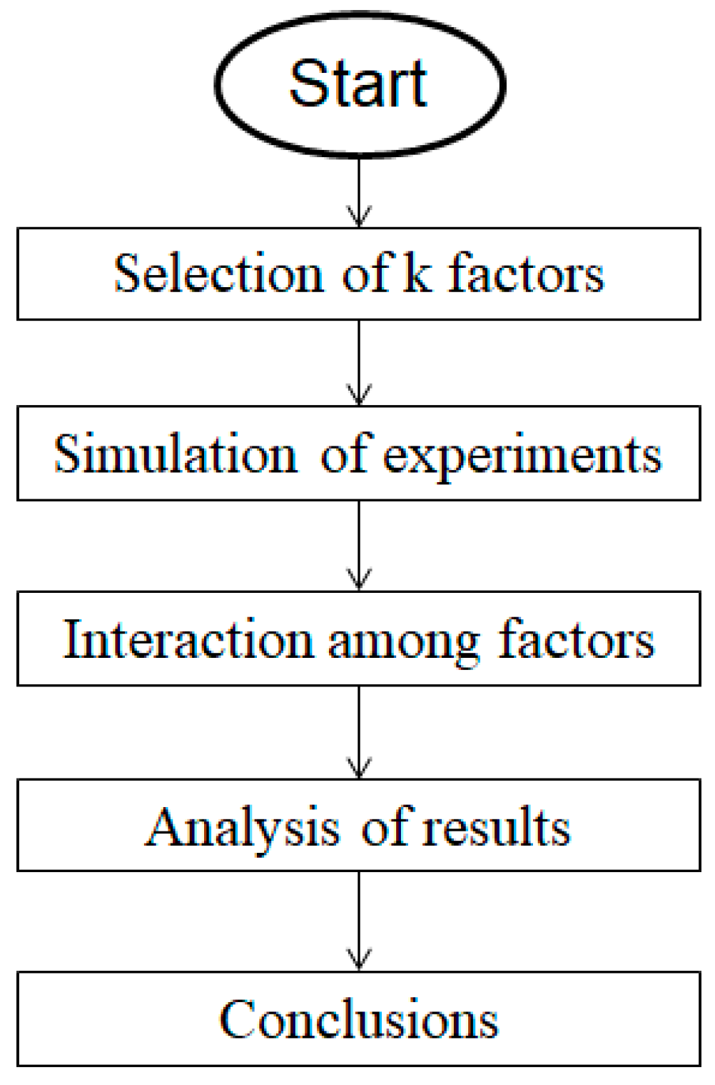
This study uses the following complete $2^k$ factorial design methodology whose flow diagram is shown in Figure 1. First, a set of $k$ interest factors is defined, determined by two critical levels (−1 and 1), for each one the them, which represent extreme values of said factors, i.e., values for the best and worst simulation scenario. Then, the experiment is run for all the $2^k$ possible combinations of factors. From each simulation $\left(\begin{array}{c}k\\ 2\end{array}\right)$ two-factor interactions are extracted, $\left(\begin{array}{c}k\\ 3\end{array}\right)$ three-factor interactions, and so on. Finally, using the sign table method the results are analyzed and the variation is assigned, depending on the combination of the different factors. A factor’s importance depends on the proportion of the total metric variation explained by the factor. The variation refers to the variance of a metric [30]. The total variation of $y$ is known as the total sum of squares (SST), which is calculated using Equation (18).

$$\mathrm{Total}\mathrm{variation}\mathrm{of} y=\mathrm{SST}={\displaystyle \sum }_{i=1}^{2^k}{\left(y_i-\overline{y}\right)}^2$$

(18)

where $\overline{y}$ denotes the mean of the responses of all the experiments. The variable $y_i$ is calculated with a non-linear regression model of the study factors. The fraction of variation explained calculates the percentage of variation or impact of a factor or combination of various study factors on a performance metric. The methodology used is described below.

3.1. Selection of k Factors

This section the study factors and performance metrics for the $2^k$ factorial analysis of the range-free and range-based localization algorithms are selected. The analysis involves two performance metrics, the MSE and the CDF of the range-free localization algorithms CL and REWL $\left(\lambda =0.15\right)$, of the range-based algorithm WLS multilateration, and of the Hyperbolic algorithm [19]. MSE and CDF performance metrics are determined by four study factors $\left(k=4\right)$, such as the path-loss exponent, the level noise, the node density, and the RNs. This selection was made base on the previous work [19,22], where the study factors determine the MSE and CDF performance metrics, through which the accuracy and precision of the localization algorithms are evaluated. The accuracy is the MSE of the position estimated and true position of the NOI throughout all the realizations [19]; this is, if $\left(x,y\right)$ is the real position of the NOI and $\left(x_i, y_i\right)$ is the estimated position of the NOI in the realization $i=1,2,\dots ,M$, this metric is given by Equation (19). The precision considers the distance error distribution, while the accuracy considers the average value of those errors [19]. When two techniques are compared, a technique with concentrated distance errors on small values is preferred.

$$\mathrm{MSE}=\frac{1}{M}{\displaystyle \sum }_{i=1}^M\left[{\left(x-x_i\right)}^2+{\left(y-y_i\right)}^2\right]$$

(19)

3.2. Simulations of Experiments

This experiment uses $\left(k=4\right)$ study factors that have an impact on the MSE and CDF, it therefore requires 16 possible combinations for each experiment. Table 3 shows the results obtained from 5000 runs for each of these combinations. The simulations were carried out MATLAB R2014a (MathWorks, Inc., Natick, MA, USA).

3.3. Interaction Among Factors

In this section, $\left(\begin{array}{c}k\\ 2\end{array}\right)$ two-study-factor interactions are used to measure the impact of the study factors on the MSE and the CDF, since the interactions of three or more study factors have no impact on the performance metrics.

4. Results

The

Table 2. Characterization of the study factors.

Symbol	Factor	Level −1	Level 1
A	Path-loss exponent $\left(\eta \right)$	$1.5$	$5$
B	Level noise $\left({\sigma }_{dB}\right)$	2 dB	10 dB
C	Node density $\left(\rho \right)$	$1\times {10}^{-4}m$	$9\times {10}^{-4}m$
D	Anchor nodes $\left(N_{rx}\right)$	5	20

shows the factors selected for this analysis and their respective critical values. Each factor is labeled with a symbol A, B, C, D and is determined by two critical levels −1 and 1 that represent extreme values of the factors defining the simulation environment.

4.1. Path-Loss Exponent

This experiment uses the log-normal shadowing model, which was used in [19,22] to evaluate the localization algorithms in the same evaluation scenario proposed for this study, as it is the most commonly used due to its simplicity and its fidelity to real Wireless Sensor and Actuator Network (WSAN) scenarios. In this model, two propagation settings are proposed with variation in the path-loss exponent $\eta$, since the frequency bands that operate in the IEEE 802.15.4 standard are a parameter that has no impact on any WSN localization scenario. The path-loss exponent $\eta$ was considered between 1.5 and 5 for this experiment, that being the typical range for WSN applications [37]. Inside a building with line of sight, the path-loss exponent $\eta =1.5$, is considered, while in obstructed in building where there is not line of sight, the path-loss exponent $\eta =5$, is considered [49].

4.2. Level Noise

In the evaluation scenario proposed in [19] the noise level was considered from 4 to 12 dB; however, in this experiment 2 and 10 dB critical levels are considered. The noise level of 2 dB represents a value that does not impact the RSS, and therefore does not affect the localization algorithms’ performance either, while a noise level of 10 dB does have a considerable impact on the performance metrics of the localization algorithms evaluated in this scenario.

4.3. Node Density

Node density describes the number of nodes distributed over an area of 100 m × 100 m considering the evaluation scenario proposed in [19,22]. Based on our references, in our experiment, the node densities of 1 and 9 nodes were used within the NOI´s coverage area of 100 m × 100 m; these numbers represent the critical node density values (minimum and maximum) over the total network area of 1000 m × 1000 m, which correspond to low and high node density, respectively.

4.4. Anchor Nodes

This is the number of nodes with a known position closest to the NOI, which are necessary to estimate the NOI’s position. For our purpose, 5 and 20 RNs are used as critical values. This experiment considered 5 RNs as the lower critical level, because experiments considering 4 or 3 RNs do not provide enough information for obtaining a precise localization, especially with range-based algorithms, which are more affected by Gaussian noise. Thus, 5 RNs were used as the lower critical level and 20 RNs as the upper critical level, since higher numbers of RNs have not been observed to increase the impact of this factor on localization.

Table 3. MSE and CDF of the localization techniques.

Levels				MSE (m)				CDF (%)
A	B	C	D	CL	REWL	Hyperbolic	WLS	CL	REWL	Hyperbolic	WLS
−1	−1	−1	−1	69.76	57.39	78.1	57.91	5.829	8.2119	9.7503	11.31
−1	−1	−1	1	127	87.85	104.45	73.04	5.663	7.5301	4.388	9.444
−1	−1	1	−1	19.23	15.91	22.94	15.94	17.68	25.452	19.241	28.15
−1	−1	1	1	26.52	18.97	28.56	16.34	15.56	22.738	11.722	27.26
−1	1	−1	−1	265.6	255.06	372.4	390.34	2.554	3.9807	1.8664	3.096
−1	1	−1	1	293.6	251.69	361.98	315.37	1.208	2.7236	0.2898	1.247
−1	1	1	−1	170.2	160.64	325.19	320.49	4.41	5.6936	4.2078	5.828
−1	1	1	1	183.2	154.97	322.31	255.76	2.296	3.5721	0.2872	3.82
1	−1	−1	−1	58.3	44.28	20.77	24.28	6.254	7.8482	23.726	25.25
1	−1	−1	1	108.2	43.61	16.63	10.19	6.29	9.2447	23.604	48.6
1	−1	1	−1	16.33	13.15	5.89	6.04	22.61	31.812	84.193	78.08
1	−1	1	1	22.86	12.42	4.49	2.94	18.31	35.898	98.97	100
1	1	−1	−1	86.24	66.16	135.69	97.77	5.506	8.1518	8.5659	8.559
1	1	−1	1	154.9	66.26	186.81	134.98	4.385	8.6823	1.8456	5.577
1	1	1	−1	24.62	19.63	43.14	33.24	13.53	19.913	12.608	16.63
1	1	1	1	32.65	18.18	62.36	30.68	12.34	22.398	6.3494	14.2

show the results obtained from the performance evaluation of the localization techniques using the MSE and CDF, respectively. To obtain the CDF values, a localization error of 10 m was considered, since for higher values of localization error a very high probability of obtaining said parameter is obtained. To obtain the MSE and CDF of the localization techniques being analyzed, four study factors are used; it therefore, 16 testing cases are required for each experiment and each case represents a specific combination of the critical levels of the study factors (A, B, C and D) as shown in Table 3.

Table 4. Impact of the study factors on the MSE and the CDF.

Factors	Variation Explained (%)
	MSE (m)				CDF (%)
	CL	REWL	Hyperbolic	WLS	CL	REWL	Hyperbolic	WLS
A	22.47	32.37	29.07	29.74	11.07	15.01	22.69	22.71
B	30.85	30.62	52.22	45.84	25.8	19.84	30.07	38.49
C	23.66	13.17	4.773	4.347	45.56	45.18	14.01	13.76
D	3.019	0.03	0.156	0.277	1.451	0.011	0.146	0.587
AB	17.68	21.48	13.18	18.25	2.622	1.821	13.86	11.14
AC	0.111	1.31	0.015	0.028	3.697	6.177	8.213	3.483
AD	0.04	0.046	0.048	0.489	0.006	0.854	0.211	1.147
BC	0.659	0.801	0.475	0.739	9.299	11.08	10.53	7.261
BD	0.000	0.113	0.021	0.26	0.006	0.022	0.215	1.425
CD	1.512	0.061	0.04	0.027	0.486	0.011	0.062	0.000

shows the percentage of variation of the performance metrics being studied for each of the study factors. A very high percentage of variation indicates that the study factor has a very high impact on the performance metric.

The results obtained from the $2^k$ factorial analysis show that:

–

The MSE and the CDF are affected to a great extent by the noise level $\left({\sigma }_{dB}\right)$, which shows a strong impact on range-based localization techniques.

–

The path-loss exponent $\eta$ has a greater impact on the MSE and the CDF of the range-based algorithms than on those of the range-free algorithms.

–

The combination of factors A and B shows greater impact on the MSE of the localization algorithms and very little on their CDF.

–

Node density $\left(\rho \right)$ has a greater impact on the MSE and the CDF of the range-free algorithms than on those of the range-based algorithms.

–

Node density $\left(\rho \right)$ is the factor that have the greatest impact on the localization algorithms’ CDF.

–

The path-loss exponent and the noise level are the factors that have the greatest impact on the localization algorithms’ MSE.

–

The number of RNs has zero impact on the range-based algorithms and shows very little impact on the CL algorithm’s MSE.

4.5. Impact of the Path-Loss Exponent.

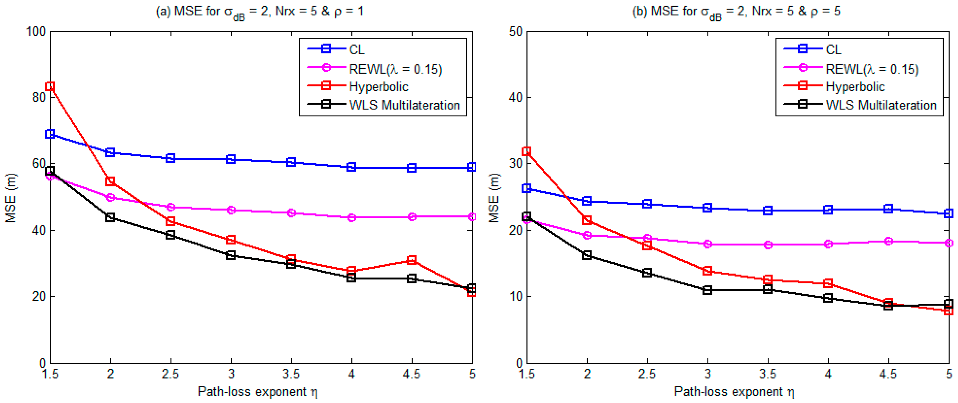
Figure 2 shows the performance graphs of the MSE as the path-loss exponent $\eta$ varies. Figure 2a shows that the Hyperbolic and Multilateration range-based algorithms show greater MSE variation than the range-free algorithms, considering a noise level $\left({\sigma }_{dB}=2\mathrm{dB}\right)$, a node density $\left(\rho =1\right)$ and 5 RNs. Figure 2b shows an increase in the node density $\left(\rho =5\right)$ and the same behavior is seen in Figure 2a. Consequently, the path-loss exponent factor shows greater impact on the range-based algorithms than on the CL and REWL range-free algorithms. According to the log-normal shadowing model, the greater the path-loss exponent, the less the RSS value is affected by the Gaussian random variable $\left({\chi }_{\sigma }\right)$, meaning that this factor has less impact on the RSS between the NOI and the RNs than on the distance separating the NOI and the RNs, which is observed using Equation (20), i.e., the error of the actual and estimated distance between the NOI and the RNs is greater than the error from the actual RSS to the estimated RSS between the NOI and the RNs. Therefore, greater localization error variation can be seen in the range-based algorithms than in the range-free algorithms, as shown in Figure 2.

$${\mathrm{RSS}}_{dB}=A-10\eta \log \left(d\right)-{\chi }_{\sigma }$$

(20)

where ${\mathrm{RSS}}_{dB}$ is the power received in dB, $A$ is the average power received at a reference distance $d_0$ and ${\chi }_{\sigma }$ is the Gaussian random variable with zero mean and standard deviation $\sigma$ in dB.

4.6. Impact of Node Density

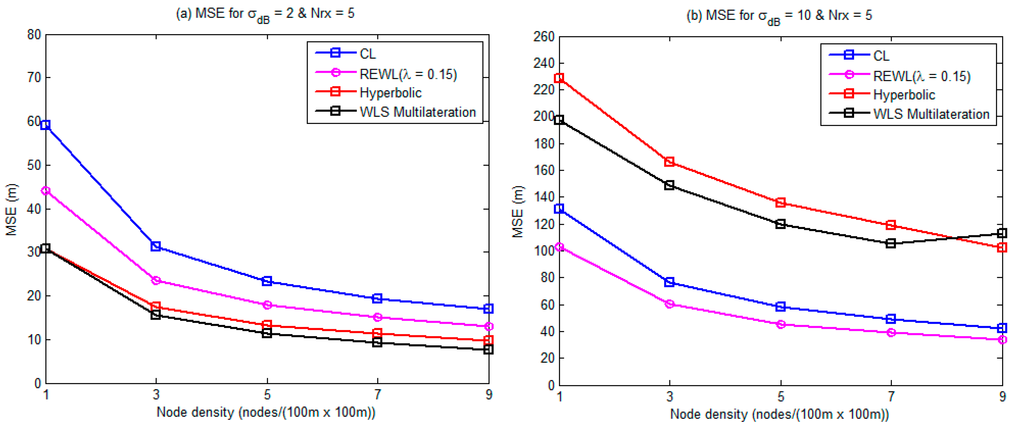
Figure 3a shows the variation of the MSE for different node densities $\left(\rho \right)$; it is evident that this study factor has greater impact on the CL and REWL range-free algorithms than on the range-based algorithms. On the other hand, Figure 3b shows that when the noise level rises $\left({\sigma }_{dB}=10\mathrm{dB}\right)$, the range-based algorithms show greater MSE variation than the range-free algorithms; thus, the noise factor has greater impact on the range-based algorithms. The results shown in Figure 3 were obtained for a path-loss exponent $\left(\eta =3\right)$. The greater the node density, the greater the RN proximity to the NOI, meaning there is less distance separating the NOI from the RNs, which reduces the NOI localization area and leads to less localization error, as shown in Figure 3 for both cases.

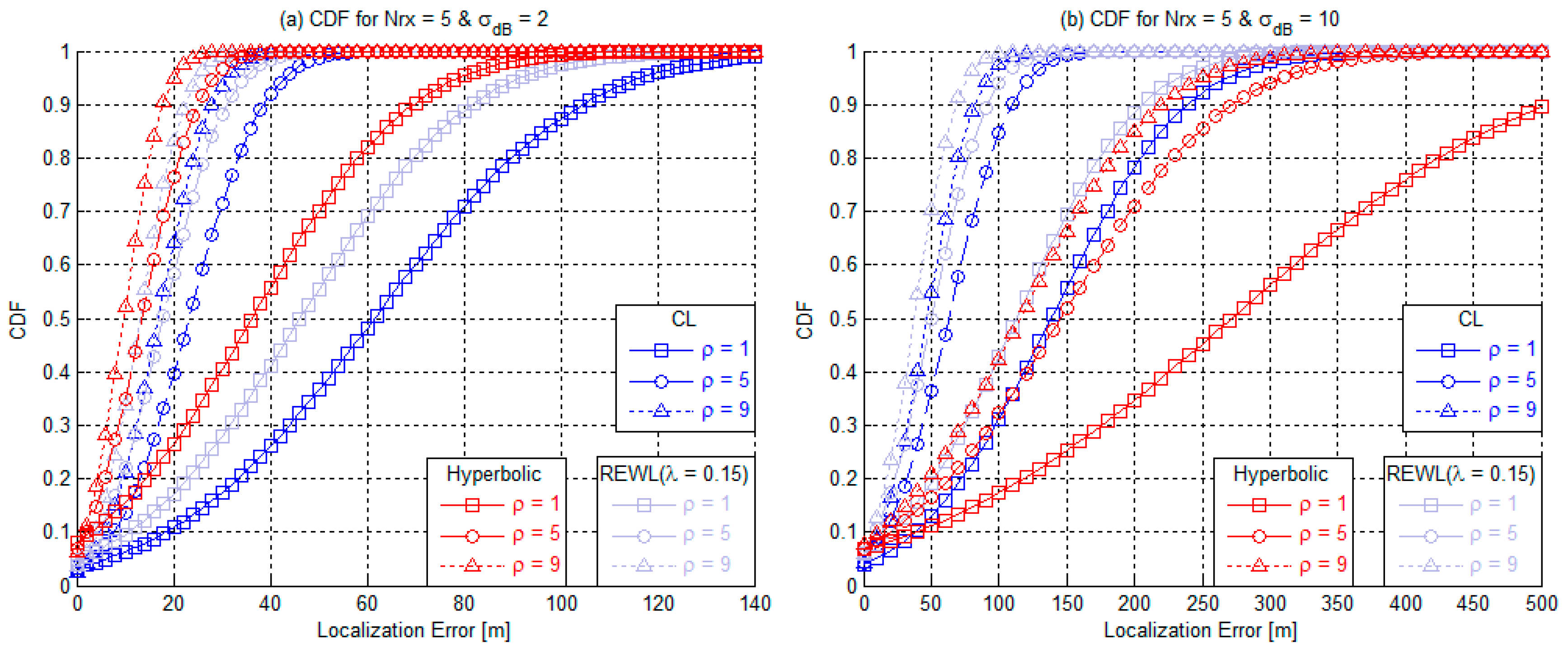
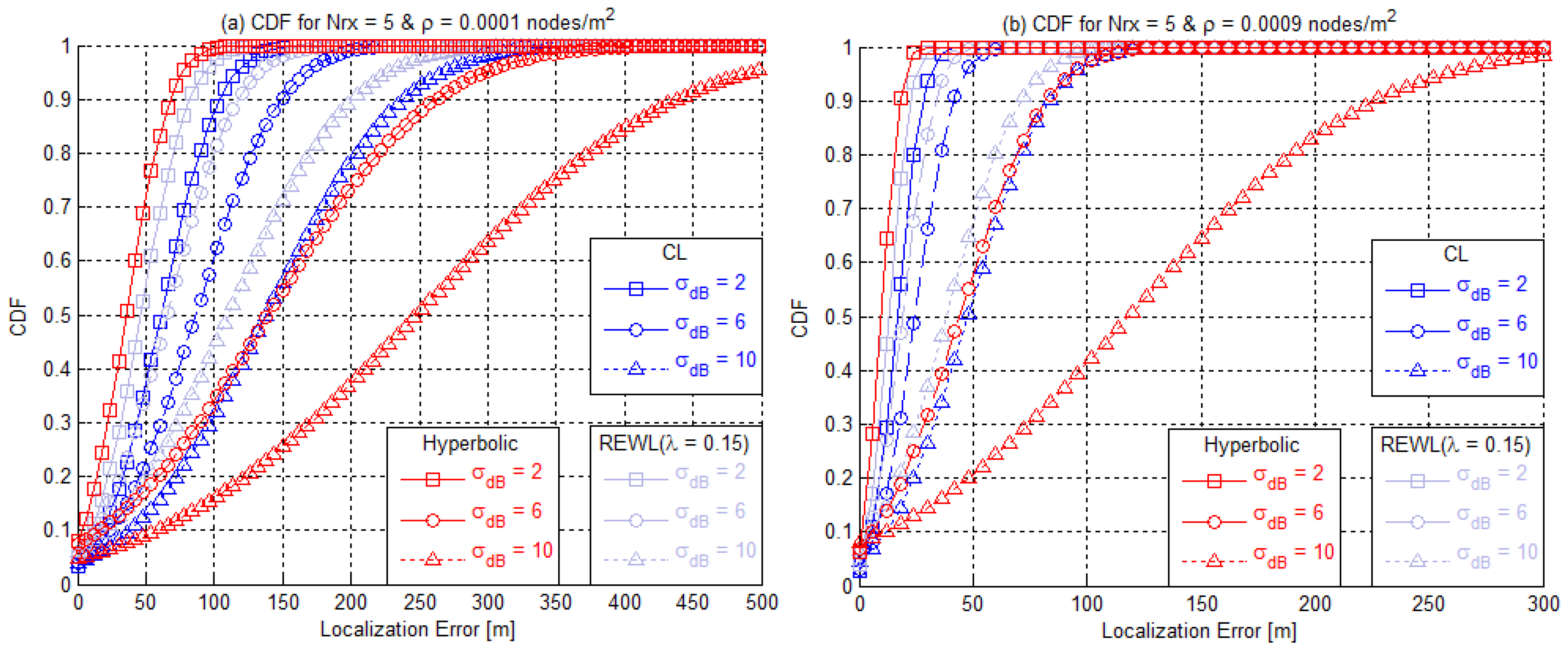
Figure 4 shows the CDF behavior of the localization techniques. As shown in Figure 4a,b, the greater the node density, the greater the CDF value of the localization techniques. Figure 4a shows that the node density $\left(\rho \right)$ has greater impact on the CL and REWL range-free algorithms considering a small noise level $\left({\sigma }_{dB}=2\mathrm{dB}\right)$, since these algorithms show greater CDF variation for different node densities. In Figure 4b the noise level increases to $\left({\sigma }_{dB}=10\mathrm{dB}\right)$ for different node densities $\left(\rho \right)$, and the noise level has greater impact on the Hyperbolic algorithm, since this algorithm shows greater CDF variation here than in Figure 4a.

4.7. Impact of Noise Level

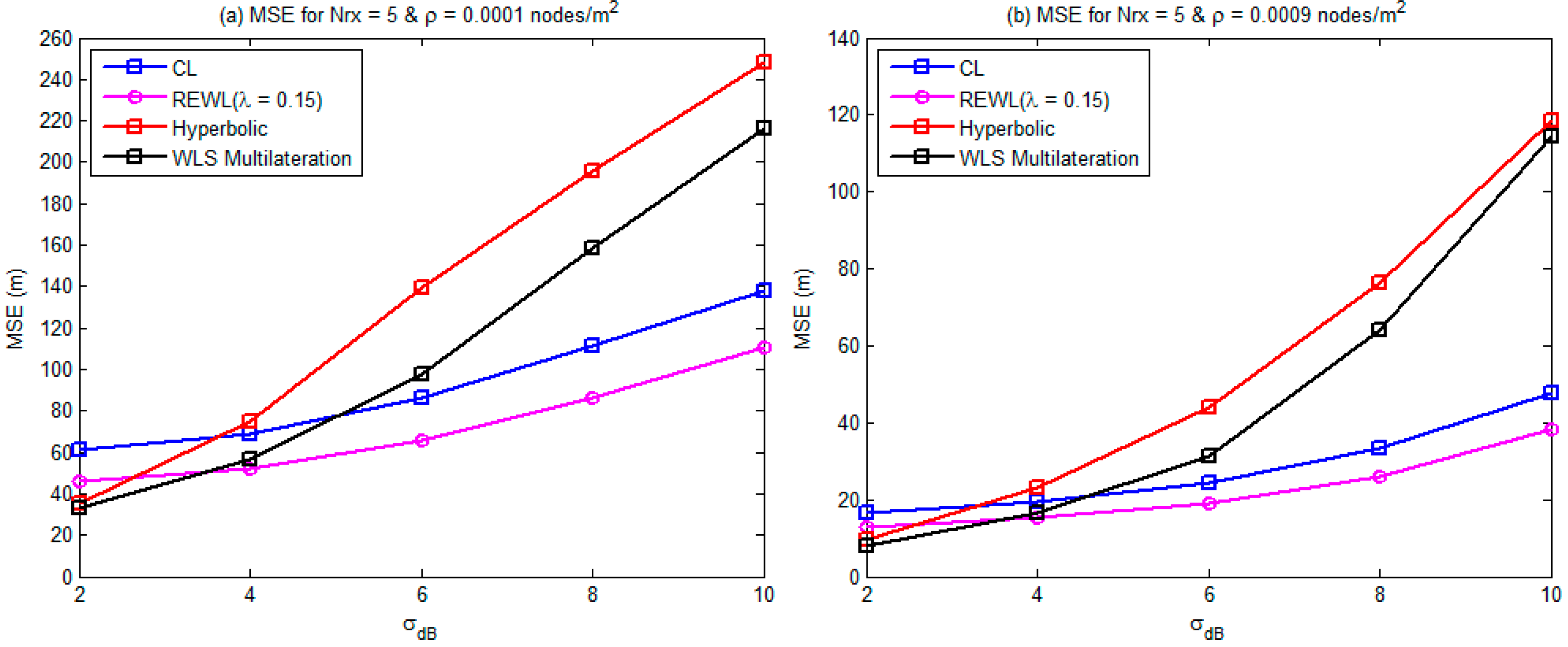
Figure 5 shows the MSE variation for different noise levels $\left({\sigma }_{dB}\right)$; this factor has greater impact on the Hyperbolic and WLS Multilateration range-based localization techniques than on the range-free localization techniques, since these algorithms show greater MSE variation for different node densities $\left(\rho \right)$. The noise level $\left({\sigma }_{dB}\right)$ is a factor that has greater impact on the distance separating the NOI from the RNs than on the RSS respectively; thus, the greater the noise level $\left({\sigma }_{dB}\right)$, the greater the error of the distance separating the NOI from the RNs, than the error of the RSS respectively, which is observed using Equation (21); therefore, the localization error is greater in the range-based localization algorithms than in the range-free algorithms, as shown for both cases in Figure 5.

$$\tilde{d}={10}^{\left(\frac{A-{\mathrm{RSS}}_{dB}}{10\eta }\right)}=d{10}^{\left(\frac{{\chi }_{\sigma }}{10\eta }\right)}$$

(21)

where $\tilde{d}$ is the separation range between the NOI and the RNs, ${\mathrm{RSS}}_{dB}$ is the power received in dB for the shadowing effects obtained in Equation (19) and $d$ is the true Euclidean distance between the NOI and the RNs.

Figure 6 shows the CDF behavior of the localization techniques. As shown in Figure 6a, the noise level has greater impact on the Hyperbolic algorithm, as this algorithm shows greater CDF variation for different node densities $\left(\rho \right)$. Figure 6b shows that the Hyperbolic algorithm shows a high level of CDF variation for high noise levels $\left({\sigma }_{dB}=10\mathrm{dB}\right)$, with a higher node density $\left(\rho =0.0009 \mathrm{nodes}/{\mathrm{m}}^2\right).$ In this figure, with low noise levels $\left({\sigma }_{dB}=2\mathrm{dB}\right)$, the CL and REWL range-free localization algorithms show greater CDF variation than the Hyperbolic algorithm, meaning that node density $\left(\rho \right)$ is a factor that shows greater impact on the range-free localization algorithms.

The results obtained show that the path-loss exponent $\left(\eta \right)$ and noise level $\left({\sigma }_{dB}\right)$ factors show greater impact on the MSE of the range-based algorithms, because as both factors increase, they have more and more impact on the error of the distance separating the NOI from the RNs while the node density shows greater impact on the MSE of the range-free algorithms. As the path-loss exponent $\left(\eta \right)$ increases, the range-based localization algorithms show less MSE than the range-free algorithms, since the range-based algorithms have greater precision in localizing the NOI. Considering high noise levels $\left({\sigma }_{dB}\right)$, the range-based localization algorithms show greater MSE than the range-free algorithms, since this factor shows greater impact on the range-based algorithms. The number of RNs is a factor that shows a very small impact on the MSE and the CDF of the localization algorithms; the results obtained show that 5 RNs are enough to localize the NOI in the proposed evaluation scenario.

5. Conclusions

This study made an analysis of the impact of the different study factors on the localization algorithms in a single-hop network, considering a simulation environment. Up to now no study has been found in the literature that looks witch factors present the most impact on the accuracy and precision metrics of localization algorithms, or on the interaction among said factors. The complete factorial method is used for the purpose of identifying the representative factors that have an impact on the accuracy and precision metrics of the localization algorithms. The performance of the localization techniques is evaluated through the accuracy and precision metrics; these performance metrics are determined using MSE and CDF, respectively. The results obtained show that the path-loss exponent $\left(\eta \right)$ and the noise level $\left({\sigma }_{dB}\right)$ factors show greater impact on the MSE and the CDF of the evaluated localization algorithms. Node density shows greater impact on the MSE and the CDF of the range-free algorithms than on those of the range-based algorithms. Finally, it can be concluded that the complete factorial method shows the magnitude of a study factor’s impact on a performance variable of the localization algorithms.

References

- Dargie, W.; Poellabauer, C. Fundamentals of Wireless Sensor Networks: Theory and Practice; John Wiley & Sons: Hoboken, NJ, USA, 2010. [Google Scholar]
- Serna, M.A.; Casado, R.; Bermúdez, A.; Pereira, N.; Tennina, S. Distributed forest fire monitoring using wireless sensor networks. Int. J. Distrib. Sens. Netw. 2015, 11, 964564. [Google Scholar] [CrossRef]
- Rawat, P.; Singh, K.D.; Chaouchi, H.; Bonnin, J.M.-S. Wireless sensor networks: A survey on recent developments and potential synergies. J. Supercomput. 2014, 68, 1–48. [Google Scholar] [CrossRef]
- Carreño, P.; Gutierrez, F.; Ochoa, S.F.; Fortino, G. Using human-centric wireless sensor networks to support personal security. In Internet and Distributed Computing Systems; Pathan, M., Wei, G., Fortino, G., Eds.; Springer: Berlin/Heidelberg, Germany, 2013; Volume 8223, pp. 51–64. [Google Scholar]
- Ali, A.; Ming, Y.; Chakraborty, S.; Iram, S. A comprehensive survey on real-time applications of WSN. Future Internet 2017, 9, 77. [Google Scholar] [CrossRef]
- Chen, S.K.; Kao, T.; Chan, C.T.; Huang, C.N.; Chiang, C.Y.; Lai, C.Y.; Tung, T.-H.; Wang, P.C. A reliable transmission protocol for Zigbee-based wireless patient monitoring. IEEE Trans. Inf. Technol. Biomed. 2012, 16, 6–16. [Google Scholar] [CrossRef] [PubMed]
- Chang, Y.-J.; Chen, C.-H.; Lin, L.-F.; Han, R.-P.; Huang, W.-T.; Lee, G.-C. Wireless sensor networks for vital signs monitoring: application in a nursing home. Int. J. Distrib. Sens. Netw. 2012, 8, 1–12. [Google Scholar] [CrossRef]
- Egbogah, E.E.; Fapojuwo, A.O. A survey of system architecture requirements for health care-based wireless sensor networks. Sensors 2011, 11, 4875–4898. [Google Scholar] [CrossRef]
- Liu, N.; Cao, W.; Zhu, Y.; Zhang, J.; Pang, F.; Ni, J. The node deployment of intelligent sensor networks based on the spatial difference of farmland soil. Sensors 2015, 15, 28314–28339. [Google Scholar] [CrossRef]
- Valente, J.; Sanz, D.; Barrientos, A.; del Cerro, J.; Ribeiro, Á.; Rossi, C. An air-ground wireless sensor network for crop monitoring. Sensors 2011, 11, 6088–6108. [Google Scholar] [CrossRef]
- Saravanan, K.A.; Balaji, D. Cracker industry fire monitoring system over cluster based WSN. J. Eng. Appl. Sci. 2014, 9, 1–5. [Google Scholar]
- Wen, T.-H.; Jiang, J.-A.; Sun, C.-H.; Juang, J.-Y.; Lin, T.-S. Monitoring street-level spatial-temporal variations of carbon monoxide in urban settings using a wireless sensor network (WSN) framework. Int. J. Environ. Res. Public. Health 2013, 10, 6380–6396. [Google Scholar] [CrossRef]
- Yang, S.; Yang, X.; McCann, J.A.; Zhang, T.; Liu, G.; Liu, Z. Distributed networking in autonomic solar powered wireless sensor networks. IEEE J. Sel. Areas Commun. 2013, 31, 750–761. [Google Scholar] [CrossRef]
- Tan, R.; Xing, G.; Chen, J.; Song, W.-Z.; Huang, R. Fusion-based volcanic earthquake detection and timing in wireless sensor networks. ACM Trans. Sens. Netw. 2013, 9, 1–25. [Google Scholar] [CrossRef]
- Dyo, V.; Ellwood, S.A.; Macdonald, D.W.; Markham, A.; Trigoni, N.; Wohlers, R.; Mascolo, C.; Pásztor, B.; Scellato, S.; Yousef, K. WILDSENSING: Design and deployment of a sustainable sensor network for wildlife monitoring. ACM Trans. Sens. Netw. 2012, 8, 1–33. [Google Scholar] [CrossRef]
- Han, G.; Xu, H.; Duong, T.Q.; Jiang, J.; Hara, T. Localization algorithms of wireless sensor networks: A survey. Telecommun. Syst. 2013, 52, 2419–2436. [Google Scholar] [CrossRef]
- Chizhov, A.; Karakozov, A. Wireless sensor networks for indoor search and rescue operations. Int. J. Open Inf. Technol. 2017, 2, 1–4. [Google Scholar]
- Cheng, L.; Wu, C.; Zhang, Y.; Wu, H.; Li, M.; Maple, C. A survey of localization in wireless sensor network. Int. J. Distrib. Sens. Netw. 2012, 8, 1–12. [Google Scholar] [CrossRef]
- Vargas-Rosales, C.; Mass-Sánchez, J.; Ruiz-Ibarra, E.; Torres-Roman, D.; Espinoza-Ruiz, A. Performance evaluation of localization algorithms for WSNs. Int. J. Distrib. Sens. Netw. 2015, 11, 493930. [Google Scholar] [CrossRef]
- Iliev, N.; Paprotny, I. Review and comparison of spatial localization methods for low-power wireless sensor networks. IEEE Sens. J. 2015, 15, 5971–5987. [Google Scholar] [CrossRef]
- Chowdhury, T.J.S.; Elkin, C.; Devabhaktuni, V.; Rawat, D.B.; Oluoch, J. Advances on localization techniques for wireless sensor networks: A survey. Comput. Netw. 2016, 110, 284–305. [Google Scholar] [CrossRef]
- Laurendeau, C.; Barbeau, M. Centroid localization of uncooperative nodes in wireless networks using a relative span weighting method. EURASIP J. Wirel. Commun. Netw. 2010, 2010, 567040. [Google Scholar] [CrossRef]
- Zanca, G.; Zorzi, F.; Zanella, A.; Zorzi, M. Experimental Comparison of RSSI-Based Localization Algorithms for Indoor Wireless Sensor Networks. In Proceedings of the Workshop on Real-World Wireless Sensor Networks, Glasgow, UK, 1–4 April 2008. [Google Scholar]
- Jose Lopez, U.; Erica Ruiz, I.; Adolfo Espinoza, R.; Joaquin Cortez, G. Implementación y Evaluación de Algoritmos de Localización Libres de Distancia. In Proceedings of the Mexican International Conference on Computer Science 2016, Chihuahua, Mexico, 14–16 November 2016. [Google Scholar]
- Janssen, T.; Weyn, M.; Berkvens, R. Localization in low power wide area networks using wi-fi fingerprints. Appl. Sci. 2017, 7, 936. [Google Scholar] [CrossRef]
- Chang, S.; Li, Y.; He, Y.; Wang, H. Target localization in underwater acoustic sensor networks using RSS measurements. Appl. Sci. 2018, 8, 225. [Google Scholar] [CrossRef]
- Yoon, H.-S. Factorial design analysis for quality of video on MANET. Int. J. Comput. Electr. Autom. Contr. Inf. Eng. 2014, 8, 446–449. [Google Scholar]
- Aragão, M.V.; Frigieri, E.P.; Ynoguti, C.A.; Paiva, A.P. Factorial design analysis applied to the performance of SMS anti-spam filtering systems. Expert Syst. Appl. 2016, 64, 589–604. [Google Scholar] [CrossRef]
- Hakak, S.; Latif, S.A.; Anwar, F.; Alam, M.K.; Gilkar, G. Effect of 3 key factors on average end to end delay and jitter in MANET. J. ICT Res. Appl. 2014, 8, 113–125. [Google Scholar] [CrossRef]
- Cano, J.C.-G.; Manzoni, P.; Sanchez, M. Evaluating the Impact of Group Mobility on the Performance of Mobile Ad Hoc Networks. In Proceedings of the 2004 IEEE International Conference on Communications, Paris, France, 20–24 June 2004. [Google Scholar]
- Singh, S.P.; Sharma, S.C. Range free localization techniques in wireless sensor networks: A review. Procedia Comput. Sci. 2015, 57, 7–16. [Google Scholar] [CrossRef]
- Mass-Sanchez, J.; Ruiz-Ibarra, E.; Cortez-González, J.; Espinoza-Ruiz, A.; Castro, L.A. Weighted hyperbolic DV-hop positioning node localization algorithm in WSNs. Wirel. Pers. Commun. 2017, 96, 5011–5033. [Google Scholar] [CrossRef]
- Zhang, S.; Li, J.; He, B.; Chen, J. LSDV-hop: Least squares based DV-hop localization algorithm for wireless sensor networks. J. Commun. 2016, 11, 243–248. [Google Scholar] [CrossRef]
- Mass-Sanchez, J.; Ruiz-Ibarra, E.; Espinoza-Ruiz, A.; Rizo-Dominguez, L. A Comparative of Range Free Localization Algorithms and DV-Hop using the Particle Swarm Optimization Algorithm. In Proceedings of the 2017 IEEE 8th Annual Ubiquitous Computing, Electronics and Mobile Communication Conference, New York, NY, USA, 19–21 October 2017. [Google Scholar]
- Sun, S.; Yu, Q.; Xu, B. A node positioning algorithm in wireless sensor networks based on improved particle swarm optimization. Int. J. Future Gener. Commun. Net. 2016, 9, 179–190. [Google Scholar]
- Vargas-Rosales, C.; Munoz-Rodriguez, D.; Torres-Villegas, R.; Sanchez-Mendoza, E. Vertex projection and maximum likelihood position location in reconfigurable networks. Wirel. Pers. Commun. 2017, 96, 1245–1263. [Google Scholar] [CrossRef]
- Munoz, D.; Bouchereau, F.; Vargas, C.; Enriquez, R. Position Location Techniques and Applications; Elsevier/Academic Press: Cambridge, MA, USA, 2009. [Google Scholar]
- Frattini, F.; Esposito, C.; Russo, S. ROCRSSI++: An efficient localization algorithm for wireless sensor networks. Int. J. Adapt. Resilient Auton. Sys. 2011, 2, 51–70. [Google Scholar] [CrossRef]
- Will, H.; Hillebrandt, T.; Yuan, Y.; Yubin, Z.; Kyas, M. The Membership Degree Min-Max Localization Algorithm. In Proceedings of the 2012 Ubiquitous Positioning, Indoor Navigation, and Location Based Service (UPINLBS), Helsinki, Finland, 3–4 October 2012. [Google Scholar]
- Xie, S.; Hu, Y.; Wang, Y. An Improved E-Min-Max Localization Algorithm in Wireless Sensor Networks. In Proceedings of the 2014 IEEE International Conference on Consumer Electronics—China (ICCE-China 2014), Shenzhen, China, 9–13 April 2014. [Google Scholar]
- Bai, E.W.; Heifetz, A.; Raptis, P.; Dasgupta, S.; Mudumbai, R. Maximum likelihood localization of radioactive sources against a highly fluctuating background. IEEE Trans. Nucl. Sci. 2015, 62, 3274–3282. [Google Scholar] [CrossRef]
- Wagh, S.S.; More, A.; Kharote, P.R. Performance evaluation of IEEE 802.15. 4 protocol under coexistence of WiFi 802.11 b. Procedia Comput. Sci. 2015, 57, 745–751. [Google Scholar] [CrossRef]
- Jawad, H.; Nordin, R.; Gharghan, S.; Jawad, A.; Ismail, M. Energy-efficient wireless sensor networks for precision agriculture: A review. Sensors 2017, 17, 1781. [Google Scholar] [CrossRef] [PubMed]
- Xiong, W.; Hu, X.; Jiang, T. Measurement and characterization of link quality for IEEE 802.15. 4-compliant wireless sensor networks in vehicular communications. IEEE Trans. Ind. Inf. 2016, 12, 1702–1713. [Google Scholar] [CrossRef]
- Yang, S.-H. Wireless Sensor Networks: Principles Design and Applications; Springer: London, UK, 2014. [Google Scholar]
- Jiang, G.; Luo, M.; Bai, K.; Chen, S. A precise positioning method for a puncture robot based on a PSO-optimized BP neural network algorithm. Appl. Sci. 2017, 7, 969. [Google Scholar] [CrossRef]
- Fogue, M.; Garrido, P.; Martinez, F.J.; Cano, J.C.-G.; Calafate, C.T.; Manzoni, P. Analysis of the Most Representative Factors Affecting Warning Message Dissemination in VANETs under Real Roadmaps. In Proceedings of the 2011 IEEE 19th International Symposium on Modeling, Analysis & Simulation of Computer and Telecommunication Systems (MASCOTS), Singapore, 25–27 July 2011. [Google Scholar]
- Delgado, R.; Hernández, C.A.M.; Solís, R.R. Applying Design of Experiments to the Design of 60 GHz Antennas for Off-Body Communications. In Proceedings of the 2016 IEEE AP-S Symposium on Antennas and Propagation and USNC-URSI Radio Science Meeting, Fajardo, PR, USA, 25 June–2 July 2016. [Google Scholar]
- Rappaport, T.S. Wireless Communications: Principles and Practice, 2nd ed.; Prentice Hall: Upper Saddle River, NJ, USA, 2010. [Google Scholar]
Figure 1.
Flowchart of the factorial design.
Figure 2.
MSE vs. Path-loss exponent .
Figure 3.
MSE vs. Node Density for different noise levels .
Figure 4.
CDF vs. Localization Error for different node densities .
Figure 5.
MSE vs. Noise level for different node densities .
Figure 6.
CDF vs. Localization Error for different noise levels .