Parsimonious Network Based on a Fuzzy Inference System (PANFIS) for Time Series Feature Prediction of Low Speed Slew Bearing Prognosis

Featured Application

The proposed method could potentially be applied in condition-based maintenance and prognosis of rotating machineries to predict the incipient and final failure.

Abstract

In recent years, the utilization of rotating parts, e.g., bearings and gears, has been continuously supporting the manufacturing line to produce a consistent output quality. Due to their critical role, the breakdown of these components might significantly impact the production rate. Prognosis, which is an approach that predicts the machine failure, has attracted significant interest in the last few decades. In this paper, the prognostic approaches are described briefly and advanced predictive analytics, namely a parsimonious network based on a fuzzy inference system (PANFIS), is proposed and tested for low speed slew bearing data. PANFIS differs itself from conventional prognostic approaches, supporting online lifelong prognostics without the requirement of a retraining or reconfiguration phase. The PANFIS method is applied to normal-to-failure bearing vibration data collected for 139 days to predict the time-domain features of vibration slew bearing signals. The performance of the proposed method is compared to some established methods, such as ANFIS, eTS, and Simp_eTS. From the results, it is suggested that PANFIS offers an outstanding performance compared to those methods.

1. Introduction

Prognosis approaches are typically applied to predict the lifetime of rotating components, which can generally be divided into two stages. The first stage refers to the normal zone, where no significant deviation from the normal operating state is observed. The second stage is the abnormal zone; this stage is initiated by potential failure that progressively develops into actual failure [1]. It is in the second stage that the prognosis methods are usually applied to predict unexpected failures on a timely basis from the impeding damage to final failure using either event data or condition monitoring (CM) data.

Steel mill industries rely on a number of rotating parts, i.e., slew bearings. These bearings support highly loaded rotation and operate at a very low speed. When unforeseen failure occurs, the steel mill industry may suffer from significant production loss. In order to predict unforeseen failure, a condition monitoring and prognosis method is required. This requirement is becoming difficult to fulfil without online real-time predictive analytics capable of delivering a reliable prediction. The prediction method for self-updating the model must be able to keep pace with non-stationary processes in typical steel mill industries due to the production target. Most processes are also subjected to a number of changing external variables. This trait cannot be handled by a static model, where its structure is fully determined in its initial design. A model is supposed to be flexible for new concepts which normally lead to the expansion of its initial structure. An over-complex structure adversely affects the model’s generalization because of overfitting. These research issues have led to algorithmic development of the so-called evolving intelligent systems (EISs) [2,3], which have attracted significant research interest over the past decade [4,5,6,7]. EISs have been successfully deployed in several predictive maintenance tasks [8,9,10].

This paper presents time-series feature prediction using a seminal work, namely the parsimonious network based on a fuzzy inference system (PANFIS) [11]. PANFIS is a fully open structure whose network structure can self-evolve during the process from data streams. PANFIS utilises the theory of statistical contribution [7,12] to prune its fuzzy rules. A unique feature of PANFIS is rgw generalized Takagi Sugeno Kang (TSK) fuzzy system, where it scatters multivariate Gaussian functions as rule premise by using the first-order TSK rule consequent. It is well-known that such rules obscure rule semantics since the atomic rules of classic fuzzy rules vanish. PANFIS is equipped with a transformation strategy which extracts a fuzzy set representation of a high-dimensional ellipsoidal cluster. The fuzzy set merging strategy is incorporated because the projection of ellipsoids to one-dimensional space normally results in overlapping fuzzy sets. The parameter learning strategy is based on the extended recursive least square method [13], which appends a binary function to enhance the convergence and stability of the tuning process.

The objective of the proposed method is to predict the future state of the slew bearing condition based on the vibration features on a timely basis. The Fuzzy-based method is selected as a prognosis method due to its capability to capture the nonlinear time-varying nature of the process [14]. Some recent literature has also proved that the fuzzy-based method is a potential method for prediction [15,16,17]. The proposed method can also be potentially applied to other time-series predictions, such as stocks prediction, climate change prediction, and tool life prediction. These examples of applications usually have a huge number of historical datasets, which are difficult to model by typical regression methods and time-series prediction methods. The challenge of the proposed method is the pre-requisite understanding of fundamental fuzzy theory, which sometimes requires an expert to determine its parameters. The PANFIS method also has high complexity in terms of programming language and parameters selection that would be another challenge to embed the proposed method into the real-time application, for example, using LabVIEW. The limitations of the proposed method are the requirement of sufficient historical datasets. Less historical datasets will reduce the prediction accuracy because the model is constructed based on minimum information from the historical datasets.

2. Classification of Prognosis Approaches

To date, there are a number of literature reviews on the prognosis approaches for rotating machineries [18,19,20,21]. For example, Lee et al. [18] reviewed prognosis methods for critical components, such as the bearing, gear, shaft, pump, and alternator. The authors classified the prognosis approaches into three types, namely model-based, data-driven, and hybrid prognosis approaches. However, the classification does not include complete methods on each prognosis approach. In their work, two methods are classified as a model-based approach, i.e., an alpha-beta-gamma tracking filter and Kalman filter, while a neural network (NN), fuzzy logic, and a decision tree are classified as a data-driven approach.

Another review paper by Jardine et al. [19] presented a clearer classification in prognosis approaches, but the review placed a greater emphasis on rotating machinery diagnostics than machinery prognostics. The authors classified the prognosis approaches into three groups: statistical, artificial intelligent (AI), and model-based approaches. The statistical approaches include statistical process control (SPC), logistic regression, autoregressive and moving average (ARMA), proportional hazard model (PHM), proportional intensity model (PIM), and hidden Markov model (HMM). In AI techniques, e.g., an artificial neural network (ANN) and its sub-classes, such as self-organising neural networks, dynamic wavelet neural networks, and recurrent neural networks, back propagation neural network and neural-fuzzy inference systems are still commonly used in AI prognostics. Among model-based approaches, defect propagation models via mechanistic modelling and the crack growth rate model are the commonly used methods.

A popular review paper on prognosis methods was presented by Heng et al. [21]. The authors classified the methodologies for predicting rotating machinery failure into two different groups, namely physics-based and data-driven prognosis models. A number of papers focusing on physics-based prognostics which used Paris’ formula are still found to be dominant [21]. Other methods, such as finite element analysis (FEA) to calculate stress and strain field, and the Forman law of linear elastic fracture mechanics, are also classified in physics-based approaches. Similar to the result from the two review papers previously mentioned, ANN and its variants are currently the most commonly used methods in the data-driven prognosis class. Other methods, such as fuzzy logic, regression analysis, particle filtering, recursive Bayesian technique, and HMM, are also included in data-driven prognosis methods. However, a number of methods within data-driven methods, as presented in [21], need further sub-classification in terms of artificial intelligent or statistical approaches.

A recent review is presented by Lei et al. [22], which mentioned that a machinery prognostic method generally consists of four technical processes, i.e., data acquisition, health indicator (HI) construction, health state (HS) division, and RUL prediction. In addition, they also explained that the existing research work and literature review have converged to the four processes, especially the latter one. The paper presents a systematic review that comprehensively covers the four technical processes.

Four prognosis approaches: (1) model-based approaches; (2) reliability-based methods and probability models; (3) data-driven approaches; and (4) combined data-driven approaches and reliability-based methods, have been developed and presented in the literature. Brief information on the prognosis methods of each approach, including the method’s name and feature, is presented in

Table 1. Prognosis methods for rolling element bearing.

No.	Classification	Method or Algorithm	Features
1	Model-based approaches: - Physics-based methods - State space-based methods	- Paris’ formula [24,25] - Stiffness-based model [26] - Kalman filter [27] - Particle filter [28]	N/A N/A N/A RMS and envelope
2	Reliability-based method and probability models:	- Gaussian process models [29] - PIM [30] - PCM 1 [31] - Stochastic model [32] - PHM [33,34] - Weibull distribution [35] - HMM [36] - WPD 2 and HMM [37]	Rényi entropy Kurtosis Principal features N/A N/A N/A RMS Peak-to-peak, energy and kurtosis
3	Data-driven approaches: - AI methods - Regression methods - AI + regression methods	- ANN [38,39] - Fuzzy logic [40] - Genetic algorithm [41] - ALE 3 and ARIMA [42] - Recursive least square [25] - Dempster-Shafer regression [43] - ARMA/GARCH 4 model [44] - RVM 5 and LR 6 [45] - RVM and exp. regression [46]	N/A N/A Monitoring index RMS, skewness, kurtosis RMS RMS and envelope RMS and envelope Kurtosis RMS
4	Data-driven + reliability-based methods	- CPH 7 model + SVM 8 [33] - (ARMA, PHM) + SVM [34] - SVM + survival probability [47] - RVM + survival probability [48] - ANN + Weibull distribution [49]	Kurtosis Peak value and RMS Kurtosis Kurtosis RMS, kurtosis and entropy estimation

¹ PCM: Proportional Covariates Model. ² WPD: Wavelet Package Decomposition. ³ ALE: Adaptive Line Enhancer. ⁴ GARCH: Generalized Autoregressive Conditional Heteroskedasticity. ⁵ RVM: Relevance Vector Machine. ⁶ LR: Logistic Regression. ⁷ CPH: Cox-Proportional Hazard. ⁸ SVM: Support Vector Machine.

. It can be seen that RMS and kurtosis are the most commonly used features in prognosis methods. It is worth noting that the reviewed methods in this paper only focused on rolling element bearings prognostics. A detailed explanation of prognosis methods classified in four approaches can be seen in [23].

3. Experimental Setup

3.1. Slew Bearing Test-Rig and Data Acquisition

The run-to-failure data used in this paper was collected from a slew bearing test rig. The test rig was designed to replicate an actual condition in steel mill manufacturing that operates the bearing in a low rotational speed, high load, and dust environment. Figure 1 shows the schematic of the slew bearing test rig, including the main drive gear reducer, the hydraulic load, and how the bearing is attached. A detailed sensors placement is presented in Figure 2. Four accelerometers, two AE sensors, and four temperature sensors were used during the experiment. Two accelerometers of IMI 608A11 ICP type sensors with a sensitivity of 100 mV/g and frequency range of 0.5 to 10 kHz, and two accelerometers of IMI 626B02 ICP type sensors with a sensitivity of 500 mV/g and frequency range of 0.2 to 6 kHz, were used. The IMI 608A11 ICP type sensors were installed on the inner radial surface at 180 degrees to each other and the IMI 626B02 ICP type sensors were attached on the axial surface at 180 degrees to each other. Similar to the measurement in continuous rotation, these accelerometers were connected to a high speed Pico scope DAQ (PS3424). The IMI 626B02 ICP type accelerometers were selected because of the minimum frequency range of 0.2 Hz and because the sensitivity is higher than that of the IMI 626B02 ICP type accelerometer. The vibration signal was acquired using a 4880 Hz sampling rate.

A three-axes (two axial rows and one radial row) brand new slew bearing is used in this experiment. Each axial and radial row has dozens of rollers inside. The slew bearing is typically large in dimension and is usually used to support a high axial and radial load [50]. The bearing attachment to the test rig is shown in Figure 1b, and 30 tonnes was applied to the bearing. The vibration signal of the bearing was acquired two times daily (morning and night). To accelerate the failure, coal dust contamination was injected into the bearing on day 90.

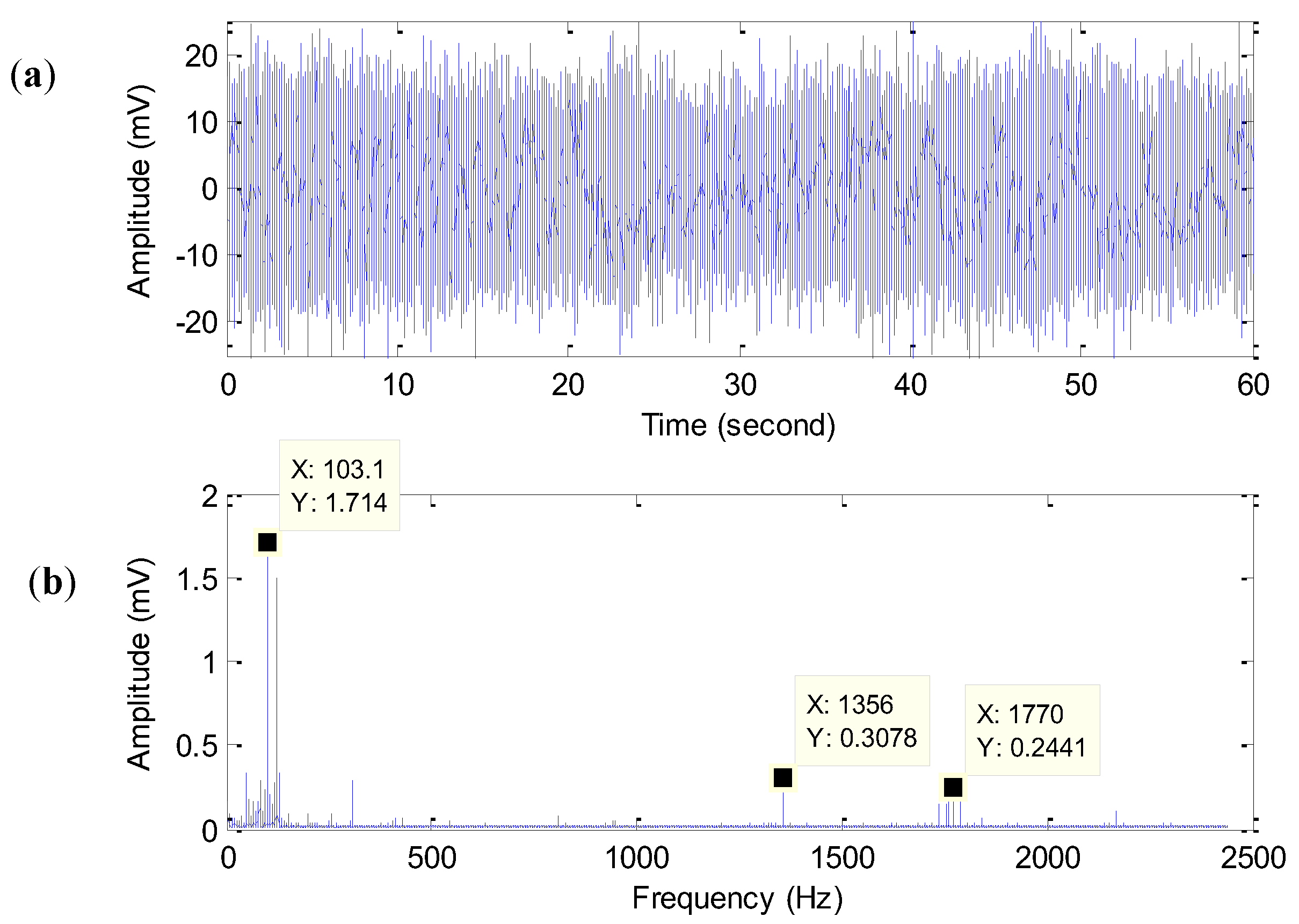
3.2. Vibration Signals

The test rig was designed to run the slew bearing from brand new until final failure. The vibration signal was monitored continuously for 139 days from February to August 2007. Each day, the vibration signal was acquired automatically using task scheduler software that automatically triggers the Pico data acquisition equipment to collect the signal for approximately 3 min. Once the vibration data are saved in the PC, a nine-features extraction executable file is also run automatically using task scheduler software at about 30 min after the digitized vibration signal is stored in the PC. An example plot of the vibration signal from accelerometer #1 (radial) is presented in Figure 3 and the feature extraction result is presented in Section 3.3.

In steel making industries, slew bearings are operated in dusty environments. Typical micro size particles from coal as the energy source in the industry are visually found inside the bearing when the bearing is dismantled from the rig during the maintenance work. In this study, the coal dust is inserted into the slew bearing to accelerate the failure in mid-April (58 days from the beginning). An example of the original vibration signal is presented in Figure 3a. The signal is collected before the final failure on 1 September. It can be seen from Figure 3b that the signal is dominated with unknown high frequency signals. None of these frequencies are associated with bearing fault frequencies. According to the FFT result, some degradation parameters, namely features, are necessary to quantitatively monitor the bearing condition, especially to identify when the impending damage occurs.

3.3. Feature Extraction

Nine time-domain features (i.e., RMS, variance, skewness, kurtosis, shape factor, crest factor, entropy, histogram upper, and histogram lower) are extracted from four sets of vibration data collected in 139 days. The example plot of nine features from accelerometer #1 (radial) is presented in Figure 4. It can be seen from Figure 4 that not all features represent the degradation condition of the slew bearing. Kurtosis, variance, and histogram lower features are more sensitive to the bearing condition than the other six features. Focusing on the RMS, variance, kurtosis, and histogram upper and histogram lower features, they show a sudden peak on day 90. This is due to the fact that coal dust has been inserted into the bearing (on day 58) and the roller and raceway have an incipient defect.

4. Parsimonious Network Based on Fuzzy Inference System (PANFIS)

This section presents the working principle of PANFIS [11]. An overview of the PANFIS learning policy is outlined in Algorithm 1 [11]. PANFIS is a modified version of the fuzzy set method, where the basic theory of the fuzzy modeling for an uncertainty nonlinear system is presented in [51]. The PANFIS algorithm is a type of evolving intelligent system (EIS) which features a fully open structure. It initiates its learning process from scratch and its fuzzy rules can be automatically generated and pruned on demand. PANFIS characterizes a generalized ellipsoidal cluster in a high dimension which arbitrarily rotates in any direction. Furthermore, PANFIS is equipped with a fuzzy set extraction strategy which allows crafting fuzzy set representation to obtain transparent traditional If-Then rules of the Takagi Sugeno Kang (TSK) fuzzy system. A fuzzy set merging scenario is incorporated to merge similar fuzzy sets. The rule consequent is constructed with a first-order linear function adjusted using the extended recursive least square (ERLS) method [13]. An architectural scheme of the PANFIS method is presented in Figure 5 and detailed steps of the PANFIS algorithm are presented in Section 4.1, Section 4.2, Section 4.3, Section 4.4 and Section 4.5.

4.1. Network Architecture of PANFIS

The unique property of PANFIS’s network architecture is observed in the presence of the multivariate Gaussian function. The multivariate Gaussian function possesses a non-diagonal covariance matrix which triggers a non-axis-parallel ellipsoidal cluster [11]. Compared to the traditional Gaussian function with the standard product t-norm operator, such a cluster offers better coverage to an irregular data distribution which does not span the main axes. As a result, it suppresses the fuzzy rule requirement to a lower level than that of the standard Gaussian rule. The multivariate Gaussian rule is, however, less transparent than the standard Gaussian rule since the atomic clause of the If-Then rule (AND-part) is omitted and thus does not have a fuzzy set representation. This calls for a transformation strategy which makes it possible to form accurate representation of a fuzzy set. The rule consequent of PANFIS is constructed under the first order TSK fuzzy rule, which is a linear function in the output space. The multivariate Gaussian function for the rule firing strength is expressed as follows:

$$R_i=\exp (-(X-C_i){\Sigma }_i^{-1}{(X-C_i)}^T)$$

(1)

where $X_n\in {\Re }^{1\times n}$ is the input feature and $C_i\in {\Re }^{1\times u}$ is the center of the multivariate Gaussian function, while ${\Sigma }_i^{-1}\in {\Re }^{u\times u}$ denotes the inverse covariance matrix which steers the orientation and size of the non-axis parallel ellipsoidal cluster. u is the input dimension. $R_i$ stands for the firing strength of the fuzzy rule, which also indicates the degree of confidence of the fuzzy rule. To guarantee the partition of unity [11], the normalization of rule firing strength is performed as follows:

$${\phi }_i=\frac{R_i}{{\displaystyle \sum _{i=1}^C{R}_i}}$$

(2)

where C is the number of fuzzy rules. The output of PANFIS results from the weighted average of the rule firing strength and the rule consequent, as follows:

$$y={\displaystyle \sum _{i=1}^C{\Omega }_i{\phi }_i=\frac{{\displaystyle \sum _{i=1}^C{\Omega }_i{R}_i}}{{\displaystyle \sum _{i=1}^C{R}_i}}}$$

(3)

where ${\Omega }_i=x_e{W}_i$ is the rule consequent of PANFIS, while $x_e\in {\Re }^{1\times (n+1)}$ and $W_i\in {\Re }^{(u+1)\times 1}$ are the extended input vector and the output weight vector of the i-th rule, respectively. The first-order TSK rule consequent is selected here because it offers a higher degree of freedom than the zero-order TSK rule consequent.

4.2. Rule Growing Mechanism of PANFIS

PANFIS uses the concept of datum significance (DS), which estimates the statistical contribution of data streams. A data point offering a high statistical contribution leads to a new rule. This concept is inspired by the neuron growing mechanism of GGAP-RBF [12] and SAFIS [6]. The key difference, however, can be found in the fact that PANFIS extends the statistical contribution concept to the framework of the multivariate Gaussian function. Suppose that a hypothetical rule (C + 1) is created using the newest data point, the DS method can be formulated as follows:

$$D_{C+1}=\left|e_n\right|\frac{{(V_{C+1})}^n}{{\displaystyle \sum _{i=1}^{C+1}{(V_i)}^n}}$$

(4)

where $e_n=\left|T_n-y_n\right|$ denotes the system error. $T_n,y_n$ refer to the target value and the predictive output at the n-th or current training observation, respectively. $V_i$ denotes the volume of the i-th rule, which can be simply calculated as the determinant of the non-diagonal covariance matrix $\det ({\Sigma }_i)$. It is seen from (4) that a datum is considered to significantly contribute to the training process provided that it causes a high system error. On the other hand, the volume of a rule portrays its zone of influence in the input space and a cluster with a small influence zone potentially contributes little during its lifespan. Note that (4) contains the implicit distance information due to the initialization of the covariance matrix. This facet addresses the novelty of the hypothetical rule because the hypothetical rule occupying a remote region possesses a high coverage span. The hypothetical rule is confirmed as a new rule if it induces high statistical contribution $D_{C+1}\ge g_1$, where $g_1$ denotes a conflict threshold. The higher the values of the conflict threshold, the lower the number of fuzzy rules added; while the lower the values of the conflict threshold, the higher the number of fuzzy rules generated during the training process.

If a new fuzzy rule is added, the center of the multivariate Gaussian function is set as the data sample of interest, while the diagonal element of inverse covariance matrix is set according to the ε-completeness principle, as follows:

$$C_{C+1}=X_N$$

(5)

$$diag({\Sigma }_{C+1}{}^{-1})=\frac{\max (\left|C_i-C_{i-1}\right|,\left|C_i-C_{i+1}\right|)}{\sqrt{\ln (\frac{1}{\epsilon })}}$$

(6)

where ε is usually set at 0.6. The ε-completeness principle borrows the seminal work of DFNN and GDFNN in [52] and [53]. It is said that there does not exist any data point with a membership degree less than ε if this setting is implemented and has been mathematically confirmed. It is worth noting that the covariance matrix of the multivariate Gaussian function is vital to the success of PANFIS. Too large values lead to averaging, while too small values lead to overfitting.

Another situation may occur during the training process where a data sample induces minor conflict. That is, the rule growing condition is not satisfied $D_{C+1}<g_1$. This triggers the so-called rule premise adaptation phase since these samples remain important to refine the network structure. The original PANFIS utilizes the evolving self-organizing map (ESOM) to update the winning rule in this situation. The underlying bottleneck of the ESOM for PANFIS rule premise adaptation is seen in the reinversion requirement, which sometimes causes instability if the covariance matrix is not in the full-rank condition. To correct this shortcoming, the direct update scheme of GENEFIS [5], and GEN-SMART-EFS [4] is adopted. The winning rule is fine-tuned if the rule growing condition is violated, as follows:

$$C_{win}=\frac{N_{win}}{N_{win}+1}{C}_{win}+\frac{(X-C_{win})}{N_{win}+1}$$

(7)

$${\Sigma }_{win}^{-1}=\frac{{\Sigma }_{win}^{-1}}{1-\alpha }+\frac{\alpha }{1-\alpha }\frac{({\Sigma }_{win}^{-1}(X-C_{win})){({\Sigma }_{win}^{-1}(X-C_{win}))}^T}{1+\alpha (X-C_{win}){\Sigma }_{win}^{-1}{(X-C_{win})}^T}$$

(8)

$$N_{win}=N_{win}+1$$

(9)

where $\alpha =1/(N_{win}+1)$ and $N_{win}$ represent the support of the winning cluster. The update of the winning rule also increases the population of the i-th cluster. The support of fuzzy rules is involved in the rule premise adaptation scheme in (7), (8) to allow stable adaptation because a cluster will converge when it is occupied by a high number of supports. This, however, calls for the forgetting mechanism in the presence of concept drift to improve the sensitivity of a highly populated cluster in accepting new training stimuli. The direct update formula of (8) is obtained from the rank-1 modification principle [5].

4.3. Rule Pruning Scenario of PANFIS

PANFIS is equipped by a rule base simplification strategy, namely the extended rule significance (ERS) method, which discards inconsequential rules. The inconsequential rules which are less important during their lifespan can be detected and will be pruned in the latter process. In the realm of EIS, the rule pruning strategy is vital to alleviate the risk of overfitting and to improve the interpretability of rule semantics. The rule pruning scenario adopts the same principle of the DS method, which approximates the statistical contribution of fuzzy rules. The ERS method is formalized as follows:

$$ER{S}_i=\left|{\delta }_i\right|\frac{{(V_i)}^n}{{\displaystyle \sum _{i=1}^C{(V_i)}^n}}$$

(10)

where ${\delta }_i={\displaystyle \sum _{j=1}^{n+1}{W}_{i,j}}$ stands for the total output weight of the i-th rule. The salient feature of the ERS method is in the approximation form of statistical contribution during the training process under the assumption of uniform distribution. In addition, (10) also measures the contribution of output weights. The fuzzy rule contribution is deemed poor provided it has a low output weight because it results in a small output which can be negligible to the overall predictive output of PANFIS. A fuzzy rule is pruned once the following condition is fulfilled:

$$ER{S}_i\le g_2$$

(11)

where $g_2$ is the rule pruning threshold. The higher the value of the rule pruning threshold, the higher the number of fuzzy rules that are pruned during the training process, and vice versa. This is because the ERS method and the DS method share a similar working principle, and $g_1,g_2$ are often selected close to each other.

4.4. Fuzzy Set Extraction and Merging Scenario

Although PANFIS operates in the high-dimensional space, it is fitted with the fuzzy set extraction scenario, which derives the fuzzy set representation of the non-axis parallel ellipsoidal cluster. This mechanism allows the classical-interpretable of the If-Then rule. The centre of the multivariate Gaussian function can be simply applied to the fuzzy set level, while the radii of the fuzzy set should be carefully determined because the ellipsoidal cluster rotates in any direction. There exist two strategies to elicit the fuzzy set radii of the multivariate Gaussian function: (1) the first method elicits the eigenvalue and eigenvector of the non-diagonal covariance matrix. The disadvantage of the first approach is its prohibitive computational cost function because of the eigenvalue and eigenvector computation, even though it offers accurate approximation; (2) the second method enumerates the distance from the center to the cutting point of the ellipsoids in the main axes. This method is computationally light, although it is rather inaccurate if the ellipsoidal cluster rotates around 45°. In such a circumstance, this method generates a spread that is too small. The present study only focuses on the second method, which is expressed as follows:

$${\sigma }_i=\frac{r}{\sqrt{{\sum }_{ii}}}$$

(12)

where $r,{\sum }_{ii}$ are the Mahalanobis distance and the diagonal elements of the covariance matrix, respectively. This mechanism is executed once completing the training process to show the fuzzy rules to operators.

PANFIS is equipped with the fuzzy set merging strategy, which aims to coalesce highly overlapping fuzzy sets. Although two fuzzy rules are well-separated in the high-dimensional space, the overlapping in fuzzy sets usually results from the projection to the one-dimensional axis. This situation often results in inconsistency of rule semantics because fuzzy rules with similar fuzzy sets generate different rule conclusions. PANFIS utilizes the kernel-based metric principle for a fuzzy set merging scenario, which compares the center and width of Gaussian fuzzy sets in one joint formula [3]. It is expressed as follows:

$$S_{\ker }(A,B)=e^{-\left|C_A-C_B\right|-\left|{\sigma }_A-{\sigma }_B\right|}$$

(13)

This formula holds the following interesting properties:

$$\begin{array}{l}{S}_{\ker }(A,B)=1\iff \left|C_A-C_B\right|+\left|{\sigma }_A-{\sigma }_B\right|\iff C_A=C_B\wedge {\sigma }_A={\sigma }_B\\ S_{\ker }(A,B)<\epsilon \iff \left|C_A-C_B\right|>\delta \vee \left|{\sigma }_A-{\sigma }_B\right|>\delta \end{array}$$

(14)

Two fuzzy sets are merged if the kernel-based metric returns $S_{\ker }(A,B)>0.8$, as set in [3]. This hyper-parameter controls a tradeoff of the intensity of the fuzzy set merging scenario, where the higher the values, the more frequently the fuzzy set merging scenario is executed, and vice versa. The fuzzy set merging process itself is carried out as follows:

$$\begin{array}{l}{c}_{new}=(\max (U)+\min (U))/2\\ {\sigma }_{new}=(\max (U)-\min (U))/2\end{array}$$

(15)

where $U=\left\{c_A\pm {\sigma }_A,c_B\pm {\sigma }_B\right\}$. This formula is used to perform the exact merging in accordance with their α-cuts. It is expected that merged fuzzy sets deliver the membership degree around 0.6, which ensures the ε-completeness at 0.6. It reflects the inflection points of Gaussian fuzzy set $c\pm \sigma$.

4.5. Adaptation of Rule Consequent

PANFIS utilizes the extended recursive least square (ERLS) method to update the rule consequent of the fuzzy rule. This approach differs from the original RLS method because of the insertion of a constant $\alpha$ to improve asymptotic convergence of the weight vector. This approach is inspired by the work presented in [13], where the system error convergence and the weight vector convergence have been mathematically proven with the help of the Lyaponov stability criterion. The constant $\alpha$ behaves like the binary function, where it is activated when the approximation error $\stackrel{⌢}{e}$ is greater than the system error $e$. It is worth mentioning that the approximation error refers to the system error before the adaptation process of one-step ahead PANFIS prediction, while the system error corresponds to after the tuning process $e_n=\left|T_n-y_n\right|$. In other words, the weight vector remains unchanged if the approximation error is lower than the system error.

$$\alpha =\{\begin{array}{l}1,\left|\stackrel{⌢}{e}\right|\ge \left|e\right|\\ 0,otherwise\end{array}$$

(16)

$$L=Q_i{x}_e{({\Psi }_i{}^{-1}+x_e{}^T{Q}_i{x}_e)}^{-1}$$

(17)

$$Q_i=(I-\alpha L{x}_e{}^T)Q_i$$

(18)

$$W_i=W_i+\alpha L(t-x_e^T{W}_i)$$

(19)

where $Q_i,L$ are the covariance matrix of the i-th rule and the Kalman gain, respectively. For the global learning scenario, the covariance matrix $Q$ is global and embraces the covariance matrix of all fuzzy rules. Since PANFIS is evolving in nature, fuzzy rules can be dynamically added Sequentially, the rule consequent is set as $W_{C+1}=W_{winner}$ if a new rule is introduced. This setting reflects where the winning rule represents the most adjacent region to the new rule. On the other hand, the covariance matrix of a new rule is set as $Q_i=\alpha I$ in the case of local learning, whereas it is assigned in the same way for the global learning case, but the dimension of the covariance matrix might have to be expanded. Note that $\alpha$ must be set as a large positive constant to assure convergence of the predictive model. The ERLS method can also be seen as a variation of the FWRLS method in [3], where the binary function is used to enhance the convergence of the adaptation process.

5. Time-Series Feature Prediction

This section presents our numerical study on the slew bearing prognosis method using the 139 data samples which correspond to 139 daily records of vibration signals. Nine input features, namely RMS, variance, skewness, kurtosis, shape factor, crest factor, entropy, histogram upper, and histogram lower, are calculated. Our simulation was carried out under two modes: direct and time-series mode.

5.1. Direct Mode Prediction

The direct mode prediction aims to study the correlation among input features, where eight features are used as the input attributes to predict the trend of input attributes. For instance, the kurtosis is made the target variable, while the other eight features serve as the input attributes to guide the predictive analytics. A schematic illustration of kurtosis feature prediction based on the PANFIS direct mode method is presented in Figure 6. This simulation aims to illustrate the descriptive power of input attributes to indicate the degradation of the slew bearing. Another goal is to model the characteristic of an input attribute based on its nonlinear relationship with the other eight input features. The 139 data points are partitioned into two groups: training and testing, where 108 samples are reserved for the training samples, while the rest are fed to test the model. In other words, prediction or testing is done for a one-month period. Figure 7 pictorially exhibits the predictive trend of PANFIS in modelling the kurtosis feature under the direct mode prediction. It is shown that the kurtosis feature characterizes a nonlinear, uncertain, and non-stationary nature; however, PANFIS is able to predict accurately. This scenario was carried out for all nine input attributes. PANFIS’s performance is examined based on its generalization power for the testing samples. It is worth noting that under the direct mode, one can observe the generalization power of PANFIS because the model is fixed after 108 days.

The evolving and adaptive characteristic of PANFIS is illustrated in Figure 8, where it shows the fuzzy rule evolution of PANFIS in the kurtosis feature prediction. PANFIS starts its learning process from no existing rules until the fuzzy rules are automatically created and pruned during the process in accordance with the novelty of data streams. PANFIS responds to changing characteristics of the system on a timely basis, where it introduces a new rule at t = 88 when there exists a “spike” in the kurtosis feature.

Table 2. Numerical results using direct partition scenario.

Input Feature	Description	PANFIS	eTS	Simp_eTS	ANFIS
RMS	RMSE (%)	0.03	0.04	0.25	0.32
	Rule	1	5	2	2
	Fuzzy set	8	40	16	16
	Time (s)	0.41	0.12	0.15	N/A
Variance	RMSE (%)	0.04	0.04	0.21	0.11
	Rule	1	5	2	2
	Fuzzy set	8	40	16	16
	Time (s)	0.43	0.13	0.15	N/A
Skewness	RMSE (%)	0.11	0.21	0.25	0.33
	Rule	8	5	2	2
	Fuzzy set	64	40	16	16
	Time (s)	0.61	0.09	0.15	N/A
Kurtosis	RMSE (%)	0.05	0.27	0.43	0.09
	Rule	1	5	2	2
	Fuzzy set	8	40	16	16
	Time (s)	0.49	0.13	1.1	N/A
Shape factor	RMSE (%)	0.006	0.05	0.11	0.33
	Rule	1	5	2	2
	Fuzzy set	8	40	16	16
	Time (s)	0.52	0.19	1.36	N/A
Crest factor	RMSE (%)	0.14	0.23	0.79	8.69
	Rule	5	5	2	2
	Fuzzy set	40	40	16	16
	Time (s)	0.35	0.1	1.29	N/A
Entropy	RMSE (%)	0.14	0.22	0.79	0.15
	Rule	5	5	2	2
	Fuzzy set	39	40	16	16
	Time (s)	0.64	0.13	1.4	N/A
Histogram upper	RMSE (%)	0.08	0.3	0.28	0.1
	Rule	1	5	2	2
	Fuzzy set	8	40	16	16
	Time (s)	0.57	0.15	1.01	N/A
Histogram lower	RMSE (%)	0.05	0.37	0.35	0.54
	Rule	1	5	2	2
	Fuzzy set	8	40	16	16
	Time (s)	0.4	0.15	1.2	N/A

presents the numerical results of consolidated algorithms in direct mode prediction. It is evident from Table 2 that PANFIS outperforms the other three algorithms in terms of predictive quality. Although ANFIS is reported to have a lower RMSE value in a few cases, it experienced 10 epochs of the training process. In addition, it is found that ANFIS suffers from the curse of dimensionality, notably when the grid partitioning method is used. Hence, two numbers of rule is selected as a fixed number in our simulations.

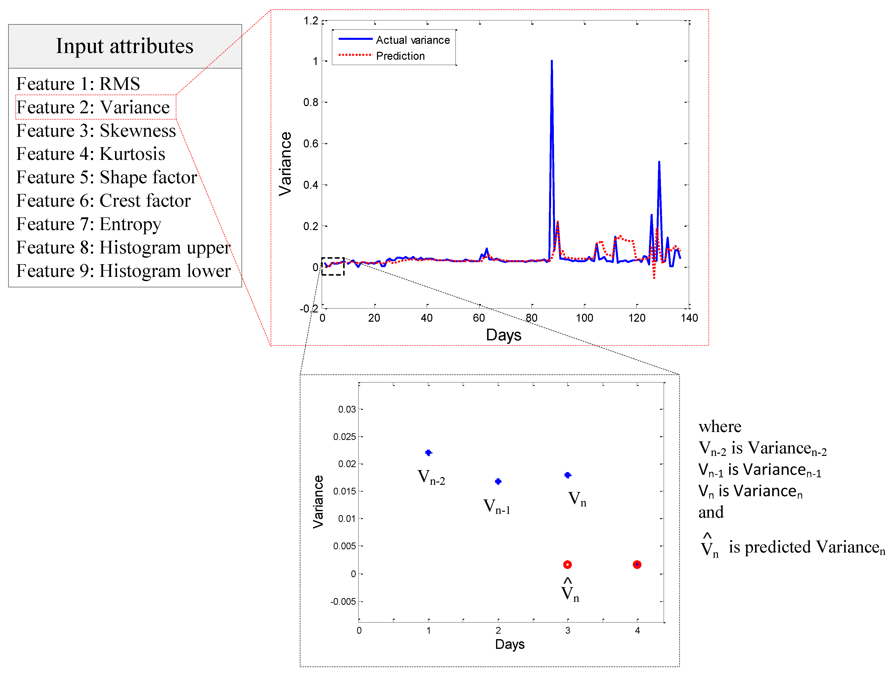
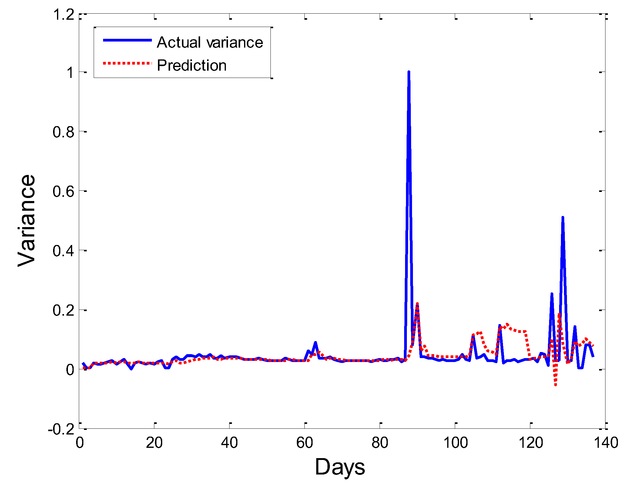
5.2. Time-Series Mode Prediction

The time-series mode aims to deliver one-step-ahead prediction based on the previous two consecutive data samples $y_n=f(y_{n-1},y_{n-2})$. The progression of the slew bearing wear is traced by the predictive model. All samples are fed to the training process and the predictive quality is evaluated by the training error, which pinpoints to what extent the predictive model learns given training representation. A schematic illustration of variance feature prediction based on PANFIS time-series mode is presented in Figure 9.

PANFIS is compared against three prominent algorithms, known as eTS [2], simp_eTS [12], and ANFIS [1]. eTS and simp_eTS are counterparts of PANFIS, which features both structural and parameter learning scenarios in the online manner. This comparison is needed to confirm the learning performance of PANFIS with respect to similar algorithms. ANFIS is a pioneer of the fuzzy neural network (FNN) which is more traditional than PANFIS, eTS, and simp_eTS. It adopts an offline learning scenario where the training process is repeated over multiple epochs. Ten epochs are applied in our study. This comparison aims to demonstrate that although PANFIS works fully in the one-pass learning scenario, it produces a comparable predictive quality.

Table 3. Numerical results using time-series scenario.

Input Feature	Description	PANFIS	eTS	Simp_eTS	ANFIS
RMS	RMSE (%)	0.1	0.11	0.13	0.1
	Rule	2	5	2	2
	Fuzzy set	2-2	5-5	2-2	2-2
	Time (s)	0.73	0.54	1.54	N/A
Variance	RMSE (%)	0.09	0.11	0.14	0.09
	Rule	6	4	2	2
	Fuzzy set	6-5	4-4	2-2	2-2
	Time (s)	1.1	0.17	1.36	N/A
Skewness	RMSE (%)	0.08	0.09	0.09	0.12
	Rule	2	5	4	2
	Fuzzy set	2-2	5-5	4-4	2-2
	Time (s)	0.78	0.12	1.42	N/A
Kurtosis	RMSE (%)	0.13	0.13	0.18	0.11
	Rule	16	6	3	2
	Fuzzy set	16-16	6-6	3-3	2-2
	Time (s)	0.49	0.09	1.72	N/A
Shape factor	RMSE (%)	0.11	0.09	0.09	0.06
	Rule	4	5	2	2
	Fuzzy set	4-3	5-5	2-2	2-2
	Time (s)	0.55	0.17	1.4	N/A
Crest factor	RMSE (%)	0.09	0.14	0.14	0.12
	Rule	3	6	7	2
	Fuzzy set	3-3	6-6	7-7	2-2
	Time (s)	0.49	0.15	2.1	N/A
Entropy	RMSE (%)	0.11	0.14	0.15	0.11
	Rule	6	6	5	2
	Fuzzy set	6-6	6-6	5-5	2-2
	Time (s)	0.51	0.12	1.81	N/A
Histogram upper	RMSE (%)	0.13	0.15	0.16	0.12
	Rule	7	8	6	2
	Fuzzy set	7-7	8-8	6-6	2-2
	Time (s)	0.69	0.19	1.7	N/A
Histogram lower	RMSE (%)	0.14	0.16	0.2	0.14
	Rule	2	8	5	2
	Fuzzy set	2-2	8-8	5-5	2-2
	Time (s)	0.52	0.15	1.5	N/A

presents the numerical results of the consolidated algorithm in time-series mode. The advantage of PANFIS is more obvious in the direct mode prediction (as shown in Table 2) than that in the time-series mode prediction, as displayed in Table 3. However, it still outperforms the other three algorithms in terms of RMSE, rule, and fuzzy set in almost all features prediction.

Figure 10 visualizes PANFIS’s prediction of the variance feature under the time-series mode. It is seen that PANFIS perfectly models the variance attribute using only its previous two time steps. Figure 8 and Figure 11 demonstrate the adaptive trait of PANFIS. It keeps changing on demand, which follows the nonlinear and time-varying properties of the given problem. PANFIS is also capable of crafting a classical-transparent fuzzy rule from a high-dimensional ellipsoidal rule through fuzzy rule transformation (14). An example of PANFIS’s rule is exemplified in variance prediction:

$$\begin{gathered} R_1:\mathbf{If}Variance=\left[\begin{array}{l}Varianc{e}_{n-1}\\ Varianc{e}_{n-2}\end{array}\right]\mathit{is}\mathit{close}\mathit{to}{C}_1=\left[\begin{array}{l}0.290\\ 0.292\end{array}\right],{\sum }_1{}^{-1}=\left[\begin{array}{l}7.4,0.19\\ 0.19,7.4\end{array}\right] \\ \mathbf{Then}y=0.03+0.17\mathrm{var}ianc{e}_{n-1}+0.04\mathrm{var}ianc{e}_{n-2} \end{gathered}$$

(20)

This fuzzy rule is rather vague and is unable to be associated directly with linguistic labels because of the absence of atomic clauses. This issue can be addressed using the fuzzy set transformation strategy (14) and this leads to the traditional expression of the fuzzy rule as follows:

$$\begin{gathered} R_1:\mathbf{If}Varianc{e}_{n-1}\mathit{is}\mathit{close}\mathit{to}{c}_{11}=0.29,{\sigma }_{11}=0.11 \\ \mathbf{and}Skewnes{s}_{n-2}\mathit{is}\mathit{close}\mathit{to}{c}_{12}=0.292,{\sigma }_{12}=0.11 \\ \mathbf{Then}y=0.03+0.17\mathrm{var}ianc{e}_{n-1}+0.04\mathrm{var}ianc{e}_{n-2} \end{gathered}$$

(21)

This rule is more readable than (20) because each fuzzy set corresponds to a specific linguistic label. This fuzzy rule is generated under the time-series mode prediction. Another example of PANFIS prediction for histogram lower feature under the time-series mode is presented in Figure 12 and the fuzzy rule evolution is presented in Figure 13.

6. Conclusions

A number of literature reviews on prognosis methods have been conducted in the last few decades and each review paper has presented its own terminology of prognosis approaches. This paper aims to consolidate all the prognosis approaches to provide a clearer understanding and guidelines in selecting the particular prognosis approach for specific needs. Following the review, a study on the time-series feature prediction has also been presented in this paper. The PANFIS-based method, which is considered as one of the data-driven prognosis approaches, is developed and presented in this paper. PANFIS provides a solution for the adaptive prognostic requirement, where it characterizes a fully open structure and operates in a single-pass learning mode. This trait makes it possible to handle non-stationary characteristics of the system in a sample-wise manner. PANFIS is tested for run-to-failure low speed slew bearing vibration data to predict the time domain vibration features. A comparative study of PANFIS and three other prominent algorithms, known as eTS, simp_eTS, and ANFIS, is also presented. It is shown that PANFIS offers a better prediction performance compared to the other three methods. In order to apply the proposed method for real-time prediction, some future research to simplify the complexity of the algorithm is necessary. A feasibility study to embed the PANFIS method into real-time measurement, for example, using the LabVIEW platform, is also expected to be conducted in the future.

References

1. Wang, W. A two-stage prognosis model in condition based maintenance. Eur. J. Oper. Res. 2007, 182, 1177–1187. [Google Scholar] [CrossRef]
2. Angelov, P.P.; Filev, D.P. An approach to online identification of Takagi-Sugeno fuzzy models. IEEE Trans. Syst. Man Cybern. Part B 2004, 34, 484–498. [Google Scholar] [CrossRef]
3. Kasabov, N.K.; Song, Q. DENFIS: Dynamic evolving neural-fuzzy inference system and its application for time-series prediction. IEEE Trans. Fuzzy Syst. 2002, 10, 144–154. [Google Scholar] [CrossRef]
4. Lughofer, E.; Cernuda, C.; Kindermann, S.; Pratama, M. Generalized smart evolving fuzzy systems. Evol. Syst. 2015, 6, 269–292. [Google Scholar] [CrossRef]
5. Pratama, M.; Anavatti, S.G.; Lughofer, E. GENEFIS: Toward an effective localist network. IEEE Trans. Fuzzy Syst. 2014, 22, 547–562. [Google Scholar] [CrossRef]
6. Rong, H.-J.; Sundararajan, N.; Huang, G.-B.; Saratchandran, P. Sequential adaptive fuzzy inference system (SAFIS) for nonlinear system identification and prediction. Fuzzy Sets Syst. 2006, 157, 1260–1275. [Google Scholar] [CrossRef]
7. Angelov, P.; Filev, D. Simpl_eTS: A simplified method for learning evolving Takagi-Sugeno fuzzy models. In Proceedings of the 14th IEEE International Conference on Fuzzy Systems, Reno, NV, USA, 25 May 2005; pp. 1068–1073. [Google Scholar]
8. Oentaryo, R.J.; Er, M.J.; San, L.; Zhai, L.; Li, X. Bayesian ART-based fuzzy inference system: A new approach to prognosis of machining processes. In Proceedings of the 2011 IEEE Conference on Prognostics and Health Management, Montreal, QC, Canada, 20–23 June 2011; pp. 1–10. [Google Scholar]
9. Pan, Y.; Er, M.J.; Li, X.; Yu, H.; Gouriveau, R. Machine health condition prediction via online dynamic fuzzy neural networks. Eng. Appl. Artif. Intell. 2014, 35, 105–113. [Google Scholar] [CrossRef]
10. Lemos, A.; Caminhas, W.; Gomide, F. Adaptive fault detection and diagnosis using an evolving fuzzy classifier. Inf. Sci. 2013, 220, 64–85. [Google Scholar] [CrossRef]
11. Pratama, M.; Anavatti, S.G.; Angelov, P.P.; Lughofer, E. PANFIS: A novel incremental learning machine. IEEE Trans. Neural Netw. Learn. Syst. 2014, 25, 55–68. [Google Scholar] [CrossRef]
12. Huang, G.-B.; Saratchandran, P.; Sundararajan, N. A generalized growing and pruning RBF (GGAP-RBF) neural network for function approximation. IEEE Trans. Neural Netw. 2005, 16, 57–67. [Google Scholar] [CrossRef] [PubMed]
13. Leng, G.; Prasad, G.; McGinnity, T.M. An on-line algorithm for creating self-organizing fuzzy neural networks. Neural Netw. 2004, 17, 1477–1493. [Google Scholar] [CrossRef] [PubMed]
14. Caesarendra, W.; Wijaya, T.; Tjahjowidodo, T.; Pappachan, B.K.; Wee, A.; Roslan, M.I. Adaptive neuro-fuzzy inference system for deburring stage classification and prediction for indirect quality monitoring. Appl. Soft Comput. 2018, 72, 565–578. [Google Scholar] [CrossRef]
15. Grzegorzewski, P. On Separability of Fuzzy Relations. Int. J. Fuzzy Log. Intell. Syst. 2017, 17, 137–144. [Google Scholar] [CrossRef] [Green Version]
16. Novak, V. Detection of Structural Breaks in Time Series Using Fuzzy Techniques. Int. J. Fuzzy Log. Intell. Syst. 2018, 18, 1–12. [Google Scholar] [CrossRef] [Green Version]
17. Rohan, A.; Rabah, M.; Kim, S.H. An Integrated Fault Detection and Identification System for Permanent Magnet Synchronous Motor in Electric Vehicles. Int. J. Fuzzy Log. Intell. Syst. 2018, 18, 20–28. [Google Scholar] [CrossRef]
18. Lee, J.; Wu, F.; Zhao, W.; Ghaffari, M.; Liao, L.; Siegel, D. Prognostics and health management design for rotary machinery systems—Reviews, methodology and applications. Mech. Syst. Signal Process. 2014, 42, 314–334. [Google Scholar] [CrossRef]
19. Jardine, A.K.S.; Lin, D.; Banjevic, D. A review on machinery diagnostics and prognostics implementing condition-based maintenance. Mech. Syst. Signal Process. 2006, 20, 1483–1510. [Google Scholar] [CrossRef]
20. Kothamasu, R.; Huang, S.H.; VerDuin, W.H. System health monitoring and prognostics—A review of current paradigms and practices. Int. J. Adv. Manuf. Technol. 2006, 28, 1012–1024. [Google Scholar] [CrossRef]
21. Heng, A.; Zhang, S.; Tan, A.C.C.; Mathew, J. Rotating machinery prognostics: State of the art, challenges and opportunities. Mech. Syst. Signal Process. 2009, 23, 724–739. [Google Scholar] [CrossRef]
22. Lei, Y.; Li, N.; Guo, L.; Li, N.; Yan, T.; Lin, J. Machinery health prognostics: A systematic review from data acquisition to RUL prediction. Mech. Syst. Signal Process. 2018, 104, 799–834. [Google Scholar] [CrossRef]
23. Caesarendra, W. Vibration and Acoustic Emission-Based Condition Monitoring and Prognostic Methods for very Low Speed Slew Bearing. Ph.D. Thesis, University of Wollongong, Wollongong, Australia, 15 December 2015. [Google Scholar]
24. Li, Y.; Billington, S.; Zhang, C.; Kurfess, T.; Danyluk, S.; Liang, S. Adaptive prognostics for rolling element bearing condition. Mech. Syst. Signal Process. 1999, 13, 103–113. [Google Scholar] [CrossRef]
25. Li, Y.; Kurfess, T.R.; Liang, S.Y. Stochastic prognostics for rolling element bearings. Mech. Syst. Signal Process. 2000, 14, 747–762. [Google Scholar] [CrossRef]
26. Qiu, J.; Zhang, C.; Seth, B.B.; Liang, S.Y. Damage mechanics approach for bearing lifetime prognostics. Mech. Syst. Signal Process. 2002, 16, 817–829. [Google Scholar] [CrossRef]
27. Lim, C.K.R.; Mba, D. Switching Kalman filter for failure prognostic. Mech. Syst. Signal Process. 2015, 52, 426–435. [Google Scholar] [CrossRef]
28. Caesarendra, W.; Niu, G.; Yang, B.S. Machine condition prognosis based on sequential Monte Carlo method. Expert Syst. Appl. 2010, 37, 2412–2420. [Google Scholar] [CrossRef]
29. Boškoski, P.; Gašperin, M.; Petelin, D.; Juričić, Đ. Bearing fault prognostics using Rényi entropy based features and Gaussian process models. Mech. Syst. Signal Process. 2015, 52, 327–337. [Google Scholar] [CrossRef]
30. Vlok, P.-J.; Wnek, M.; Zygmunt, M. Utilising statistical residual life estimates of bearings to quantify the influence of preventive maintenance actions. Mech. Syst. Signal Process. 2004, 18, 833–847. [Google Scholar] [CrossRef]
31. Sun, Y.; Ma, L.; Mathew, J.; Wang, W.; Zhang, S. Mechanical systems hazard estimation using condition monitoring. Mech. Syst. Signal Process. 2006, 20, 1189–1201. [Google Scholar] [CrossRef]
32. Wang, W. A model to predict the residual life of rolling element bearings given monitored condition information to date. IMA J. Manag. Math. 2002, 13, 3–16. [Google Scholar] [CrossRef]
33. Caesarendra, W.; Widodo, A.; Yang, B.S. Combination of probability approach and support vector machine towards machine health prognostics. Probab. Eng. Mech. 2011, 26, 165–173. [Google Scholar] [CrossRef]
34. Tran, V.T.; Pham, H.T.; Yang, B.S.; Nguyen, T.T. Machine performance degradation assessment and remaining useful life prediction using proportional hazard model and support vector machine. Mech. Syst. Signal Process. 2012, 32, 320–330. [Google Scholar] [CrossRef] [Green Version]
35. Yang, F.; Xiaodiao, H.; Jie, C.; Hua, W.; Rongjing, H. Reliability-based residual life prediction of large-size low-speed slewing bearings. Mech. Mach. Theory 2014, 81, 94–106. [Google Scholar]
36. Zhang, X.; Xu, R.; Kwan, C.; Liang, S.Y.; Xie, Q.; Haynes, L. An integrated approach to bearing fault diagnostics and prognostics. In Proceedings of the 2005 American Control Conference, Portland, OR, USA, 8–10 June 2005; pp. 2750–2755. [Google Scholar]
37. Ocak, H.; Loparo, K.A.; Discenzo, F.M. Online tracking of bearing wear using wavelet packet decomposition and probabilistic modeling: A method for bearing prognostics. J. Sound Vib. 2007, 302, 951–961. [Google Scholar] [CrossRef]
38. Shao, Y.; Nezu, K. Prognosis of remaining bearing life using neural networks. Proc. Inst. Mech. Eng. Part I J. Syst. Control Eng. 2000, 214, 217–230. [Google Scholar] [CrossRef]
39. Gebraeel, N.; Lawley, M.; Liu, R.; Parmeshwaran, V. Residual life predictions from vibration-based degradation signals: A neural network approach. IEEE Trans. Ind. Electron. 2004, 51, 694–700. [Google Scholar] [CrossRef]
40. Jantunen, E. Prognosis of rolling bearing failure based on regression analysis and fuzzy Logic. J. Vib. Eng. Technol. 2006, 5, 97–108. [Google Scholar]
41. Li, D.Z.; Wang, W. An enhanced GA technique for system training and prognostics. Adv. Eng. Softw. 2011, 42, 452–462. [Google Scholar] [CrossRef]
42. Kosasih, B.; Caesarendra, W.; Tieu, K.; Widodo, A.; Moodie, C.A.S. Degradation trend estimation and prognosis of large low speed slewing bearing lifetime. Appl. Mech. Mater. 2014, 493, 343–348. [Google Scholar] [CrossRef]
43. Niu, G.; Yang, B.S. Dempster-Shafer regression for multi-step-ahead time-series prediction towards data-driven machinery prognosis. Mech. Syst. Signal Process. 2009, 23, 740–751. [Google Scholar] [CrossRef]
44. Pham, H.T.; Yang, B.S. Estimation and forecasting of machine health condition using ARMA/GARCH model. Mech. Syst. Signal Process. 2010, 24, 546–558. [Google Scholar] [CrossRef]
45. Caesarendra, W.; Widodo, A.; Yang, B.S. Application of relevance vector machine and logistic regression for machine degradation assessment. Mech. Syst. Signal Process. 2010, 24, 1161–1171. [Google Scholar] [CrossRef]
46. Maio, F.D.; Tsui, K.L.; Zio, E. Combining relevance vector machines and exponential regression for bearing residual life estimation. Mech. Syst. Signal Process. 2012, 31, 405–427. [Google Scholar] [CrossRef]
47. Widodo, A.; Yang, B.S. Machine health prognostics using survival probability and support vector machine. Expert Syst. Appl. 2011, 38, 8430–8437. [Google Scholar] [CrossRef]
48. Widodo, A.; Yang, B.S. Application of relevance vector machine and survival probability to machine degradation assessment. Expert Syst. Appl. 2011, 38, 2592–2599. [Google Scholar] [CrossRef]
49. Ali, J.B.; Chebel-Morello, B.; Saidi, L.; Malinowski, S. Accurate bearing remaining useful life prediction based on Weibull distribution and artificial neural network. Mech. Syst. Signal Process. 2015, 56–57, 150–172. [Google Scholar]
50. Caesarendra, W.; Tjahjowidodo, T. A review of feature extraction methods in vibration-based condition monitoring and its application for degradation trend estimation of low-speed slew bearing. Machines 2017, 5, 21. [Google Scholar] [CrossRef]
51. Jafari, R.; Yu, W. Fuzzy modeling for uncertainty nonlinear systems with fuzzy equations. Math. Probl. Eng. 2017, 2017, 1–10. [Google Scholar] [CrossRef]
52. Wu, S.; Er, M.J. Dynamic fuzzy neural networks-a novel approach to function approximation. IEEE Trans. Syst. Man Cybern. Part B 2000, 30, 358–364. [Google Scholar]
53. Wu, S.; Er, M.J.; Gao, Y. A fast approach for automatic generation of fuzzy rules by generalized dynamic fuzzy neural networks. IEEE Trans. Fuzzy Syst. 2001, 9, 578–594. [Google Scholar]
Figure 1. (a) Slew bearing rig picture; (b) Schematic of laboratory slew bearing rig showing a slew bearing attached in the drive ring and the applied load from the hydraulic.
Applsci 08 02656 g001
Figure 2. A detailed sketch of the location of four accelerometers and two AE sensors on slew bearing.
Applsci 08 02656 g002
Figure 3. Slew bearing vibration signal on 30 August 2007: (a) 1 min duration signal; (b) FFT.
Applsci 08 02656 g003
Figure 4. Time-domain feature extraction results (139 days).
Applsci 08 02656 g004
Figure 5. An architectural scheme of the PANFIS method.
Applsci 08 02656 g005
Figure 6. A schematic diagram of direct mode prediction.
Applsci 08 02656 g006
Figure 7. PANFIS prediction of kurtosis feature.
Applsci 08 02656 g007
Figure 8. Fuzzy rule evolution of kurtosis feature.
Applsci 08 02656 g008
Figure 9. A schematic diagram of time series mode prediction.
Applsci 08 02656 g009
Figure 10. PANFIS prediction of variance feature.
Applsci 08 02656 g010
Figure 11. Fuzzy rule evolution of variance feature.
Applsci 08 02656 g011
Figure 12. PANFIS prediction of histogram lower feature.
Applsci 08 02656 g012
Figure 13. Fuzzy rule evolution of histogram lower feature.
Applsci 08 02656 g013