Development of an Efficient Numerical Method for Wind Turbine Flow, Sound Generation, and Propagation under Multi-Wake Conditions

Abstract

The propagation of aerodynamic noise from multi-wind turbines is studied. An efficient hybrid method is developed to jointly predict the aerodynamic and aeroacoustics performances of wind turbines, such as blade loading, rotor power, rotor aerodynamic noise sources, and propagation of noise. This numerical method combined the simulations of wind turbine flow, noise source and its propagation which is solved for long propagation path and under complex flow environment. The results from computational fluid dynamics (CFD) calculations not only provide wind turbine power and thrust information, but also provide detailed wake flow. The wake flow is computed with a 2D actuator disc (AD) method that is based on the axisymmetric flow assumption. The relative inflow velocity and angle of attack (AOA) of each blade element form input data to the noise source model. The noise source is also the initial condition for the wave equation that solves long distance noise propagation in frequency domain. Simulations were conducted under different atmospheric conditions which showed that wake flow is an important part that has to be included in wind turbine noise propagation.

1. Introduction

The generation and propagation of wind turbine aerodynamic noise exhibit several special characteristics as compared to some other industrial noise problems. Considering the generation of wind turbine aerodynamic noise, the rotor aerodynamic noise level depends on airfoil profiles at cross sections, blade shape (the spanwise distribution of chord, twist, and airfoils), rotor size, rotational speed, yaw angle, tilt angle, pitch setting, the angular position of blades, wind speed profile, inflow turbulence level, density, and viscosity of air. From the perspective of aerodynamic noise propagation (ANPropagation), aerodynamic noise source (ANSource) of large wind turbines is often located at high altitude which leads to more significant problem for ANPropagation over long range. Intrinsically, the study of wind turbine noise is a multi-disciplinary subject which should consider wind farm aerodynamic noise generation (ANGeneration), ANPropagation, and energy production. However, ANGeneration from a single airfoil has a similar basis in the nature of aerodynamics and aeroacoustics as that from a large wind farm. Sophisticated numerical methods are needed to understand the physical mechanisms of flow induced noise. Computational aero-acoustics (CAA) methods were widely applied favored by the high-performance computing technology. However, advanced large eddy simulation (LES)/CAA method still requires heavy computational effort. Consequently, conventional CAA methods are neither efficient to model wind farm noise source, nor to predict long range ANPropagation. In the following paragraphs, feasible aerodynamic and aero-acoustic modeling techniques are briefly reviewed and the numerical methods employed in the current study are introduced.

As a prerequisite for wind turbine noise source and propagation modeling, a proper aerodynamic tool should be considered. There are many methods developed for wind turbine aerodynamic simulations. The classic blade element momentum (BEM) method [1,2] is a commonly used semi-engineering technique that simulates the aerodynamics of a single wind turbine. With a BEM model, one can apply engineering approaches to compute the noise source level of a wind turbine. When the prediction accuracy increases, the model complexity as well as the computational cost also increases. It is known that the CFD based methods predict the rotor aerodynamic forces and the wake flow behind the rotor more accurately. Considering long-distance ANPropagation of wind turbines, CFD methods become time consuming because the wake flow should be simulated in the large range whose size is the same as that of the ANPropagation. In the present study, the velocity field is the input data for the ANPropagation solver. Instead of conventional CFD methods, other sophisticated methods are developed for wind turbine applications, such as the AD/AL/AS (actuator disc /actuator line /actuator surface) methods, these methods have good trade-off between model accuracy and computational efficiency. The actuator disc method [3,4] is applied in this study which has relatively high computational efficiency. The rotor is assumed as a permeable disc. The aerodynamic loadings of the rotor are treated as external volume force terms of the momentum equations of Navier–Stokes (NS) equations. The rotor disc of a horizontal axis wind turbine (HAWT) has an inherent axisymmetric characteristic. In this study, to reduce computational time the 3D-AD method is simplified to 2D-AD. The boundary condition of rotor center is axisymmetric, such that the obtained flowfield with 2D-NS equations will be exactly identical to that of the 3D case. Since the axisymmetric assumption is made, it has to be mentioned that the solution only holds correct for axisymmetric uniform inflow conditions and rotor under no yaw and tilt manipulations.

Dealing with the modeling of ANSource, the CAA methods, based on high fidelity techniques [5,6,7,8,9,10], can model the physical details of flow induced noise mechanisms. Nevertheless, the atmospheric acoustic scientists mainly focus on sound propagation problems with larger scales or sizes [11,12,13]. It is true that the governing equations of most CAA based methods can solve both wind turbine ANGeneration and ANPropagation problems, but the heavy simulation cost often limits the computational domain into small size. It is clear that more efficient methods with less computational effort are needed. To satisfy this requirement, the flow passing wind turbine, the ANSource and the ANPropagation through long path are naturally combined together in this study. The engineering ANSource model for wind turbine [14,15,16] is built into the above mentioned AD flow solver. Such that the relative inflow velocity and AOA of each blade section are obtained from the AD-CFD simulation and then fed into the noise source model of wind turbine.

Afterwards, the relative sound pressure level (RSPL) from wind turbines is simulated over large distances from the turbine positions to the desired receivers. The wind turbine ANSource are the key inputs to the propagation solver [11,12]. The wind turbine wake flow, computed by the AD-CFD method, is considered as the medium of ANPropagation. The complex flow environment is found as an important factor for long-path wind turbine ANPropagation. In the previous study of Lee [17] and Heimann [18], the influences of atmospheric conditions on ANPropagation were investigated. Both studies showed that there is large noise variation under different wind profile and atmospheric stability conditions. More recently, this parabolic equation (PE) method is used by Barlas et al. [19,20] for wind turbine noise applications. It was clearly shown that the wind turbine ANPropagation has different refraction characteristics under various wake conditions. The present work focuses on an integrated method for modeling of flow, ANSource and ANPropagation, and the detailed phenomenon of ANPropagation through multi-wind turbine wakes are studied.

This paper is organized following the sequences: In Section 2, the numerical method for wind turbine flow simulation, ANGeneration and ANPropagation modeling are described; Section 3 provides results of various validation cases first and more results from the integrated flow-noise model afterwards; conclusions are provided in the last section.

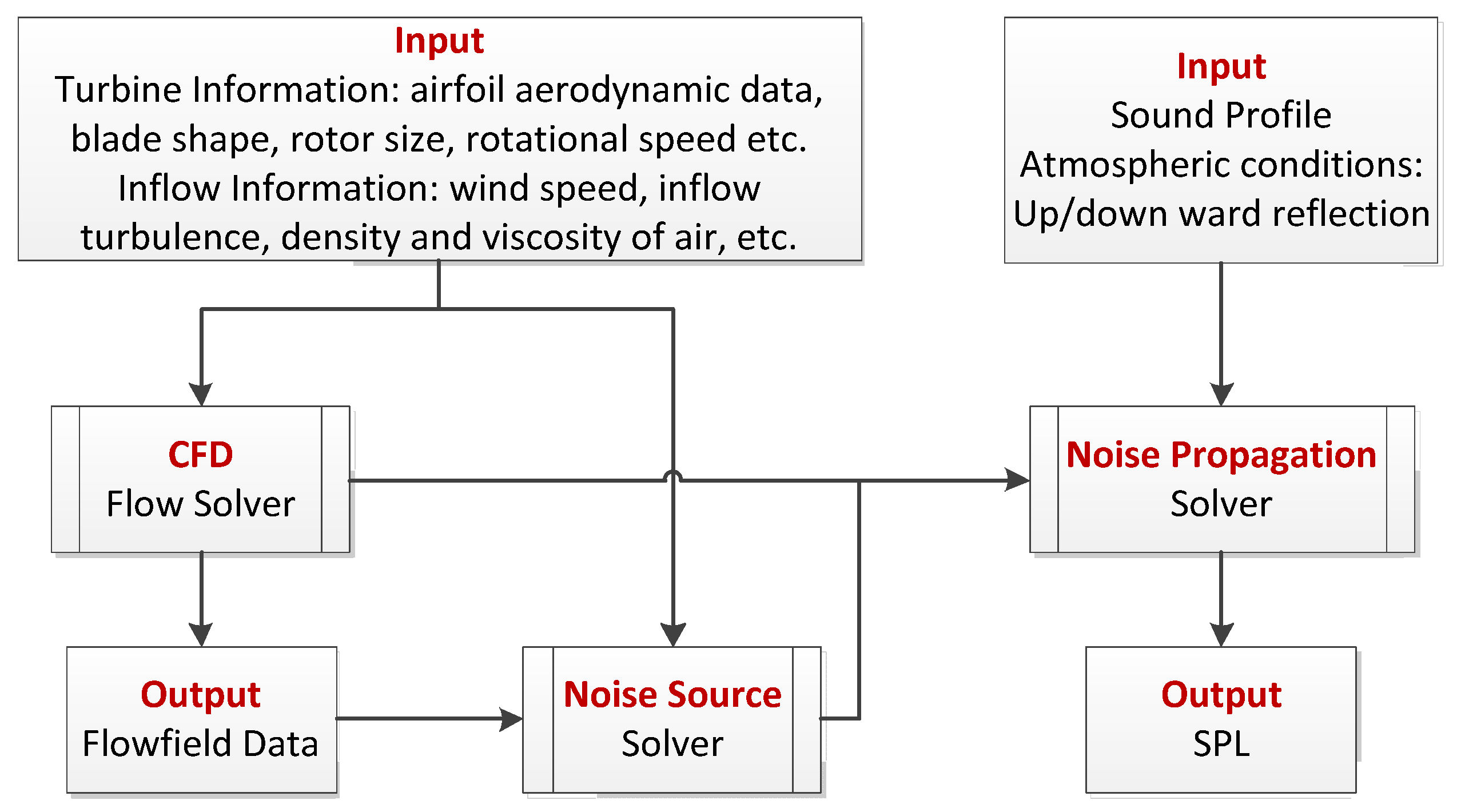
2. Numerical Methods

The related numerical methods applied in the study are described separately in this section: (1) The RANS/AD model for wind turbine flow simulation; (2) The BPM (named after Brooks TF, Pope DS, Marcolini MA [14]) wind turbine ANGeneration model; (3) The wind turbine ANPropagation model. The relations between the solvers are shown in the schematic diagram below in Figure 1. It is seen that the flowfield data are the input to both the wind turbine noise source and propagation models.

2.1. RANS/AD Method

To simulate the flow passes wind turbine rotor, the general equations are modified by adding the aerodynamic loadings of the rotor as external volume force terms in the momentum equations of the NS equations

$$\frac{\partial u_i}{\partial x_i}=0 (i=1 , 2 )$$

(1)

$$\frac{\partial u_i}{\partial t}+u_j\frac{\partial u_i}{\partial x_j}=-\frac{1}{\rho }\frac{\partial P}{\partial x_i}+\frac{\partial }{\partial x_j}(\nu \frac{\partial u_i}{\partial x_j}-\overline{{u^{\prime }}_i{u^{\prime }}_j})+f_{ext}$$

(2)

$$-\rho \overline{{u^{\prime }}_i{u^{\prime }}_j}={\mu }_t\left(\frac{\partial u_i}{\partial x_j}+\frac{\partial u_j}{\partial x_i}\right)-\frac{2}{3}\rho k{\delta }_{ij}$$

(3)

where $x_i$ is the displacement in the inertial coordinate system and $u_i$ is the velocity components. t, $\rho$, and P represent time, air density and pressure respectively. $\nu$ is the kinematic viscosity term, $f_{ext}$ is the added source term. With the assumption based on the axisymmetric property of the HAWT, 2D-RANS/AD method is utilized such that the computational effort can be greatly decreased.

The rotor is assumed as permeable disc such that the mass equation remains unchanged. To avoid numerical instability the volume force in Equation (2) should be smeared along the flow direction using 1D Gaussian function. For the elements which are away from the disc with a normal distance of d, the smeared force f’ is computed by convolution computation

$$f\prime =f_{AD}\otimes {\eta }^{1D}$$

(4)

$${\eta }^{1D}(d)=1/\left(\epsilon \sqrt{\pi }\right)\exp \left[-{(d/\epsilon )}^2\right]$$

(5)

where the free parameter $\epsilon =3\Delta z$ is three times larger than the axial size of reference grid $\Delta z$. What is more, the body forces of rotor can be computed using blade element theory with the aerodynamic data of airfoil and the simulated information of flowfield.

The present 2D-AD method solves the ideal axisymmetric flowfield. The axial and tangential induced velocities are naturally combined with the NS equations, such that the inflow angle and the relative inflow velocity are determined from

$$\varphi ={\tan }^{-1}\left(\frac{V_0-W_z}{\mathsf{\Omega }r+W_{\theta }}\right), V_{rel}^2={\left(V_0-W_z\right)}^2+{\left(\mathsf{\Omega }r+W_{\theta }\right)}^2$$

(6)

The local AOA is easily computed by $\alpha =\varphi -\gamma$, where $\gamma$ is the real twist angle (added by pitch) at local blade element. The lift and drag forces per unit span are computed using Equation (7) with the aerodynamic data of airfoil.

$$L=\frac{1}{2}\rho V_{rel}^{2}cB{C}_l, D=\frac{1}{2}\rho V_{rel}^{2}cB{C}_d$$

(7)

The blade forces are updated after each iteration using newly computed velocity field, then the external volume force terms of the NS equations apply renewed blade forces in the next iteration.

2.2. BPM Model for Noise Source or Generation

The original BPM noise model was developed by Brooks et al. [14] which is able to predict airfoil self-noise. The model was based on scaling the wind tunnel experimental data using the NACA 0012 airfoil with chord lengths varies from 2.5 cm to 61 cm. Here, the BPM model was integrated with the BEM method [15] in order to deal with the complicated flow for wind turbine. The required boundary layer thickness data in the BPM model is obtained from the Xfoil computation so that this data varies with the airfoils rather than fixed with NACA 0012. A general expression of the BPM model is shown in Equation (8)

$$\mathrm{SPL}=10lo{g}_{10}\left(\frac{\delta M^{n}lD}{r^2}\right)+G_1\left(St\right)+G_2\left(Re\right)+G_3\left(\delta \right)+C$$

(8)

In the equation, it is shown that rotor aerodynamic noise is mainly a function of parameter $\delta$ which represents boundary layer thickness. The boundary layer thickness depends on airfoil shape, Reynolds number, AOA, turbulence level etc. l is the spanwise length of an airfoil segment. G₁, G₂, and G₃ are related to the Strouhal number St, Mach number M, Reynolds number Re and boundary layer thickness parameter $\delta$. Detailed descriptions of noise mechanisms can be found in references [14,15]. ANSource level of rotor generally depends on the blade shape and operational conditions, such as rotational speed, wind speed, yaw, tilt, etc. Instead of combining the engineering BEM model, the BPM noise model is directly integrated into the NS equations with the AD model. The BPM model is a passive subroutine that can be activated anytime with the inflow velocity and AOA provided from AD simulations. The trailing edge boundary layer thickness is interpolated from the existing database prepared with Xfoil through a wide range of Reynolds numbers and AOAs. To take clean and rough blade surface conditions into account, the boundary layer thickness database is created under different surface roughness cases, such that wind turbine noise under free transition and fully turbulent flows can be modelled. A fully-turbulent boundary layer thickness database is utilized to calculate the noise of rotor whose blade surface is rough, and free transition database is applied for a rotor with a clean surface.

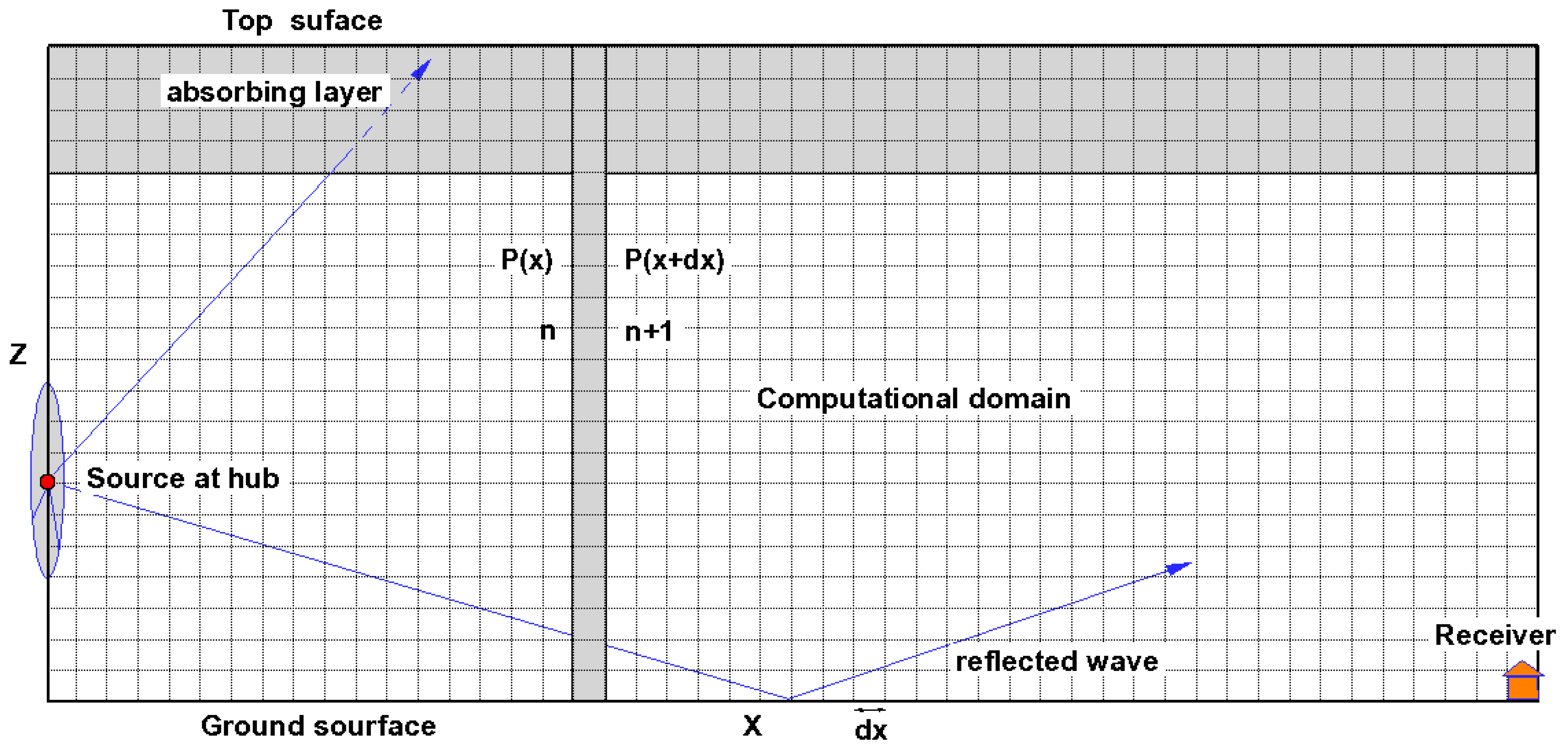
2.3. Noise Propagation Method

Sound speed in an ambient flow is written as $c_{eff}=c+v_x$ where c is the constant sound speed at a given air temperature, $v_x$ is the wind speed component through the propagation path. The wind speed components may come from field measurements, empirical expressions or numerical simulations. For an incompressible wind flow, the air density is assumed as a constant, the wave equation in a moving atmosphere reads [12]

$$\left[{\nabla }^2+k^2\left(1+ϵ\right)-\frac{2i}{\omega }\frac{\partial v_i}{\partial x_j}\frac{{\partial }^2}{\partial x_i\partial x_j}+\frac{2ik}{c_0}\mathit{v}\cdot \nabla \right]P^{\prime }\left(r\right)=0$$

(9)

where $k=\omega /c_0$, $\omega$ is the radian frequency of sound wave, $c_0$ is the reference sound speed, $P^{\prime }\left(r\right)$ denotes the monochromatic field of sound pressure and $\epsilon ={(c_0/c)}^2-1$. If the effect from ambient flow is neglected, this equation can be further reduced to Helmholtz equation. The ANSource of a wind turbine is placed on the left boundary of the computational domain depicted in Figure 2. A classical approach to represent a monopole ANSource is to distribute the source along the vertical direction which is also called starting field. In this study, the rotor noise source is located at the hub height as sketched at the left side of the boundary. Based on the initial source strength, the equation or the sound pressure amplitude is computed along the x-direction, such that solution is renewed from P(x) to P(x + Δx). The boundary condition applied on the ground surface is calculated from the impedance of the ground. The empirical impedance model for absorbing materials developed by Delany and Bazely [21] is used in this study,

$$Z=1+0.0511{\left(\frac{\sigma }{f}\right)}^{0.75}+i 0.0768{\left(\frac{\sigma }{f}\right)}^{0.73}$$

(10)

where Z is the normalized acoustic impedance, $\sigma$ represents the flow resistivity and f is the frequency. The similar approach can be applied on the top surface. A constant of the normalized acoustic impedance Z = 1 is implemented on the top grid, such that the vertical waves through the top surface is vanished without any reflection. However, to sufficiently eliminate wave reflections, an absorbing layer is defined on top of the grid. As shown in the figure, the grey region sketched on top of the domain is the absorbing layer. In the study, the width of such an absorbing layer is defined as 50$\lambda$. This implies that for lower frequency sound propagation, a larger absorbing layer is needed. The sound pressure along the vertical line is updated from step n to n + 1 until the receiver position is reached. The solution procedure starts with the separation of the forward and backward propagation waves. Here, only the forward wave propagates from source towards receiver is considered (in the positive x-axis), which is in the downwind direction. Detailed mathematical manipulations of the equation are found in [12,13].

According to the methodologies described in Section 2.1 and Section 2.2, the noise spectrum of a given wind turbine is the logarithmic sum of sound pressure level (SPL) from all the blade elements such that

$$L_p\left(f\right)=10lo{g}_{10}\left({\displaystyle \sum }_i^n{10}^{0.1SP{L}_{total}^i}\right)$$

(11)

where n is the number of the blade elements and $SP{L}_{total}^i$ is the SPL of the ith blade element, which accounts for all the noise mechanisms. The SPL of wind turbine ANSource $L_p\left(f\right)$ is the initial condition for calculating long-path ANPropagation. The sound power level $L_w\left(f\right)$, which is a representation of wind turbine total noise strength, it does not change with propagation range. The SPL at the receiver is

$$L_p\left(f\right)=L_w\left(f\right)-10lo{g}_{10}4\pi D^2-\alpha D+\Delta L$$

(12)

where the first term on the right side is the sound power level, the second term $-10{\log }_{10}4\pi D^2$ is the geometric attenuation term that corresponds to the sound intensity loss when the sound wave sphere is expanding. The third term shows the attenuation due to air absorption, which is proportional to the absorption coefficient $\alpha$ and the propagation length D. $\Delta L$ is the relative SPL differences caused by factors such as ground reflection/absorption (flat/irregular terrain), atmospheric refraction, wind and turbulence and sound barriers, etc. It does not include the effects of geometric attenuation and air absorption. The $\Delta L$ varies along the propagation path with these factors, which is beneficial to clearly manifest the effects of propagation. Most of the discussions and results in Section 3 are dealing with this relative pressure level which is abbreviated as RSPL. The values of $\alpha$ depend on sound frequency, air temperature, pressure and humidity. In the following studies, unless specified separately, a relative humidity of 70% and temperature of 10 °C are assumed.

The wave equation is solved based on each frequency. The ANSource and wake information of given wind turbines from BPM/AD computations are combined into the ANPropagation solver. For each frequency, the corresponding ANSource, known as the starting field, is individually applied as the initial condition to the computational domain. Detailed descriptions about starting field formulation can be found in publication from Salomons [11]. The horizontal size of the simulation range is determined by the location of the receiver. However, the size of the vertical domain is flexible such that the height of domain can vary with the simulated frequency. The maximum vertical size of the grid should be less than $\Delta x=\Delta z=\lambda /8$ so that a sound wave can be resolved with at least eight grid points. As a result, the domain height is inversely proportional to frequencies for a fixed number of vertical grids. Besides, a larger CFD domain should be used in the simulation such that the flow field can fully cover the noise propagation domain.

3. Results and Discussions

A few validations about ANPropagation cases are shown first. Under various flow conditions, the flow passing wind turbine rotor, ANGeneration and ANPropagation problems are discussed in detail. The RSPL $\Delta L$ over a long distance is computed for each frequency. After the validations, the wind turbine ANPropagation across multi-wakes is shown. In all the cases, the temperature at the ground level is 15 °C, such that the equivalent sound speed is 340 m/s.

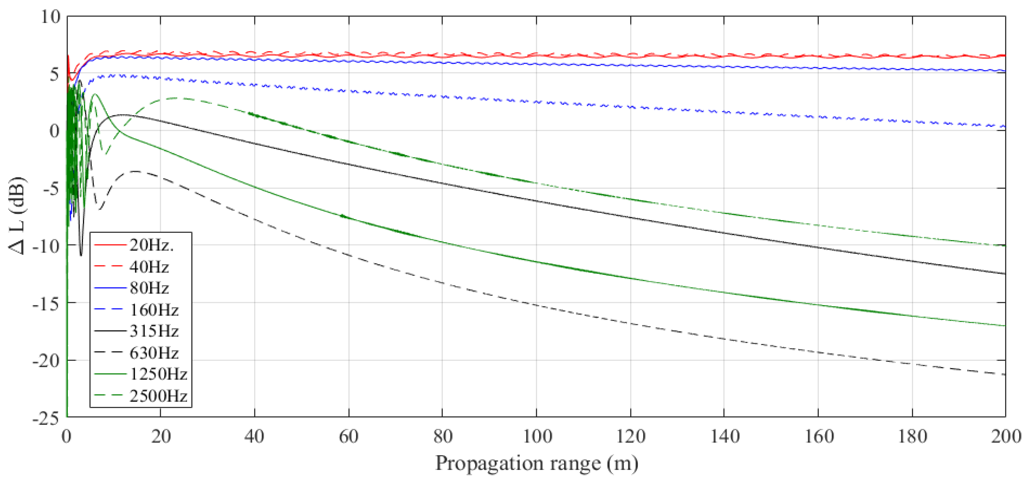
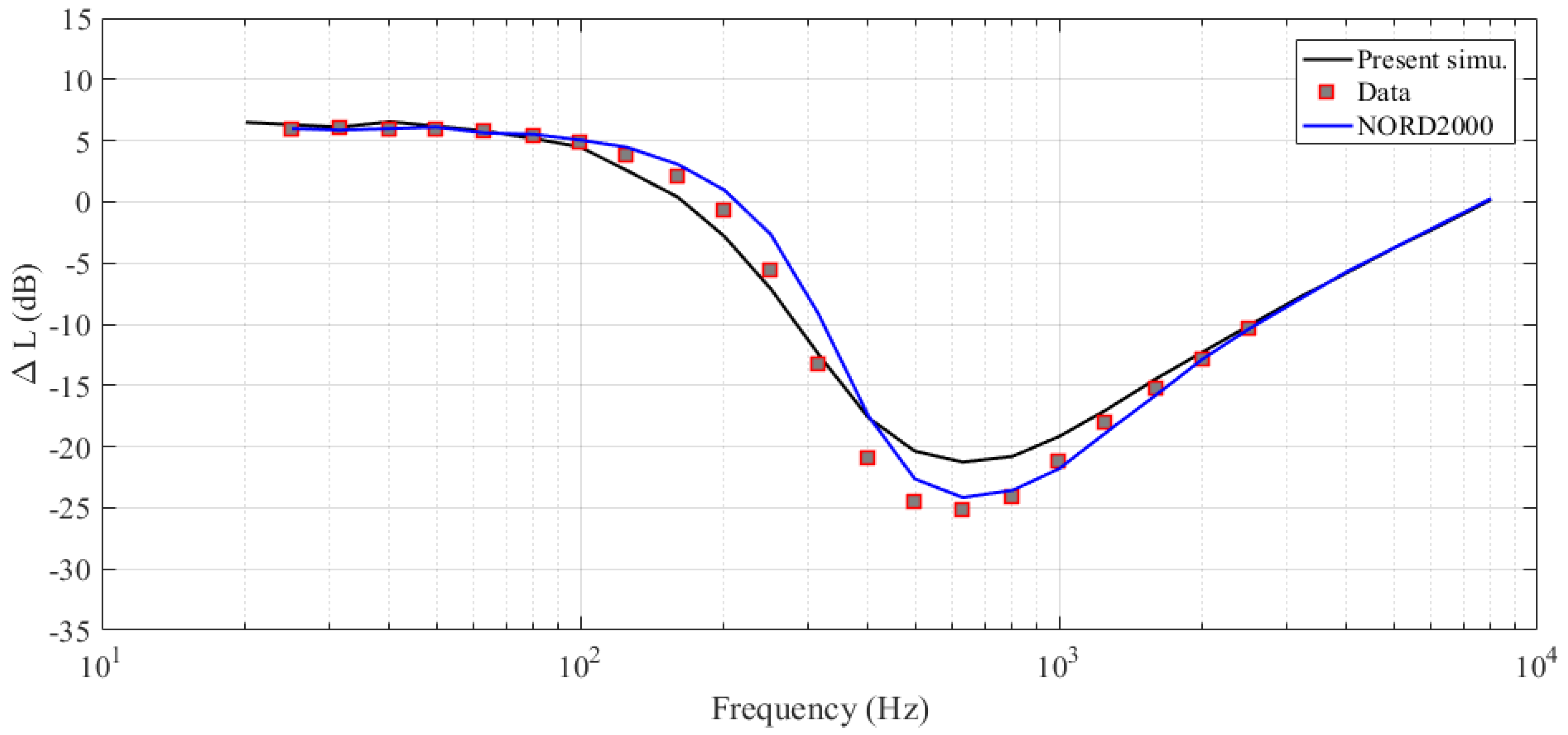
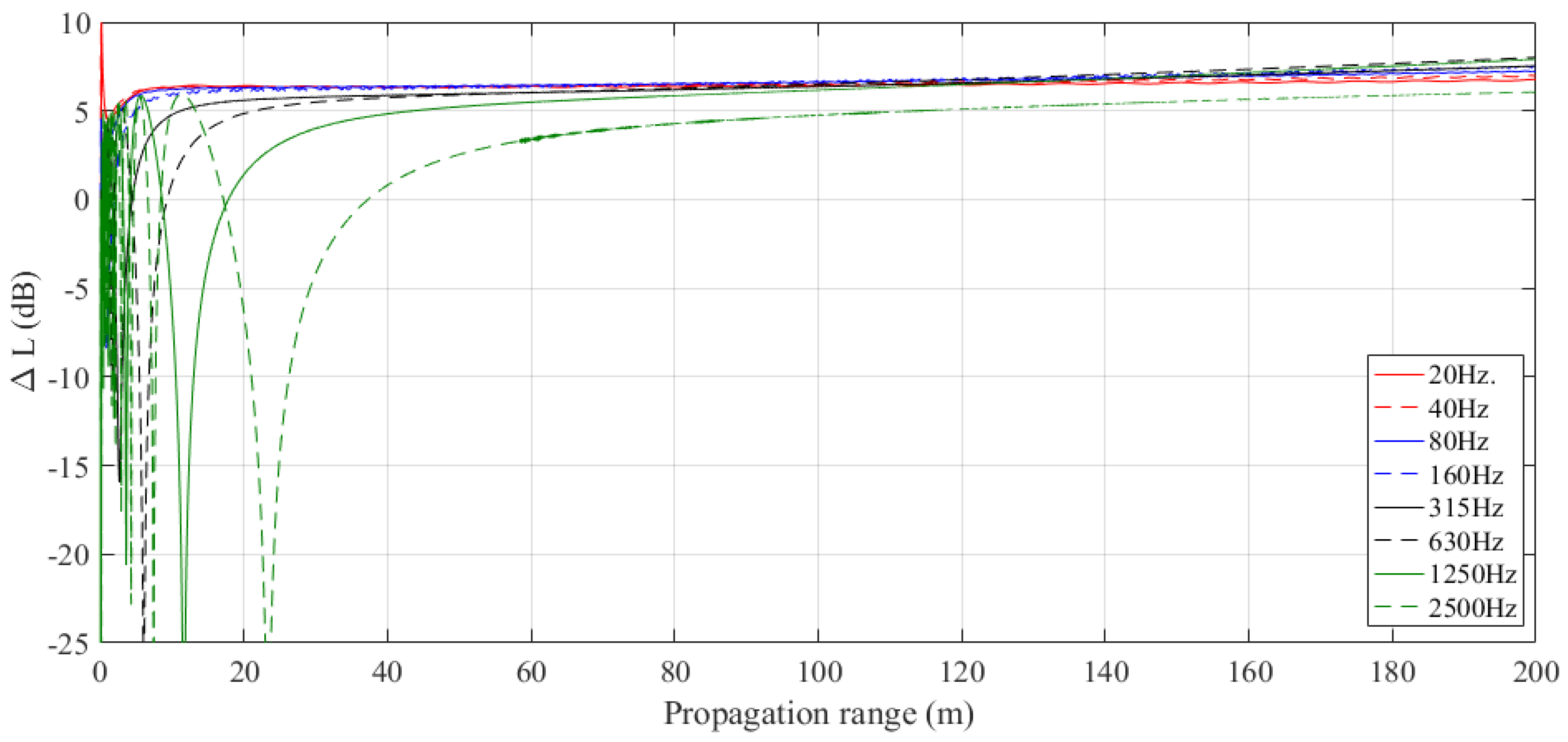
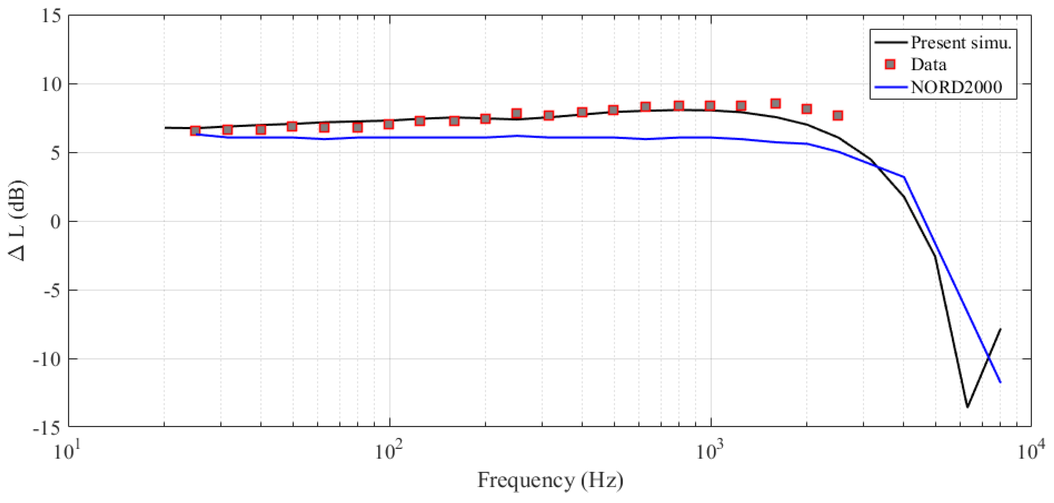
3.1. Validation of Long-Range Sound Propagations without Ambient Flow

This validation case considers the idealized long-range sound propagation without any moving medium or temperature gradient effects. The terrain contains a flat and acoustically soft surface with a total length of 200 m. The flow resistivity of a grassland are usually in range from 100 $\mathrm{kPa}\cdot \mathrm{s}\cdot {\mathrm{m}}^{-2}$ to 300 $\mathrm{kPa}\cdot \mathrm{s}\cdot {\mathrm{m}}^{-2}$. The absorbing ground surfaces in the current simulation has a flow resistivity of 250 $\mathrm{kPa}\cdot \mathrm{s}\cdot {\mathrm{m}}^{-2}$. The ANSource locates at x = 0 m, z = 0.5 m and the receiver at x = 200 m, z = 1.5 m. The current results are compared with the data presented in reference [22] where either measured data or data obtained from other models are available. The sound transmission losses over 200 m are shown in Figure 3 where the selected frequencies in the 1/3-octave band are gathered. At very low frequencies, i.e., f = 20 Hz and f = 40 Hz, the RSPL $\Delta L$ is increased with the propagation distance. At higher frequencies, $\Delta L$ gradually decreases along the propagation distance. The $\Delta L$ values at 200 m are compared in Figure 4 which shows that there is a large propagation loss between 400 Hz and 1000 Hz. The present simulation agrees with the reference data and the simulation obtained from the Nord2000 commercial model [23].

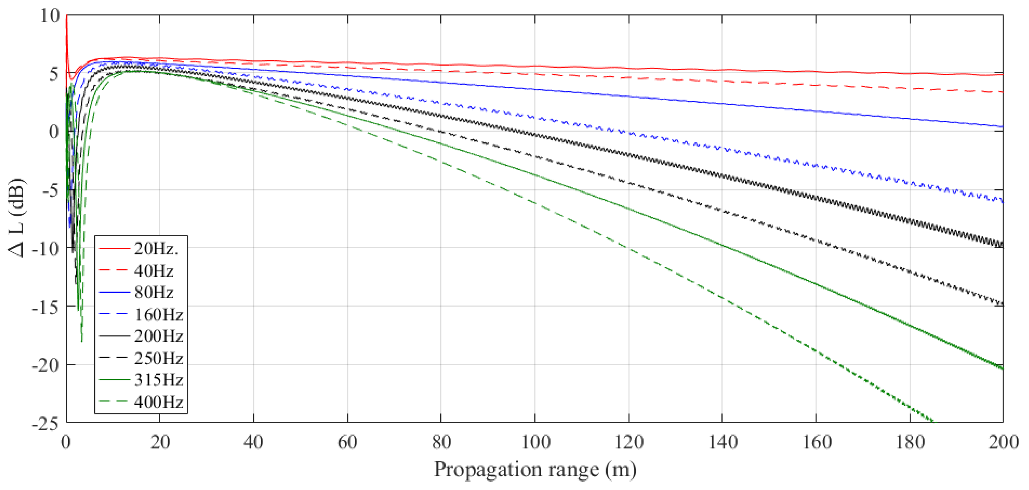
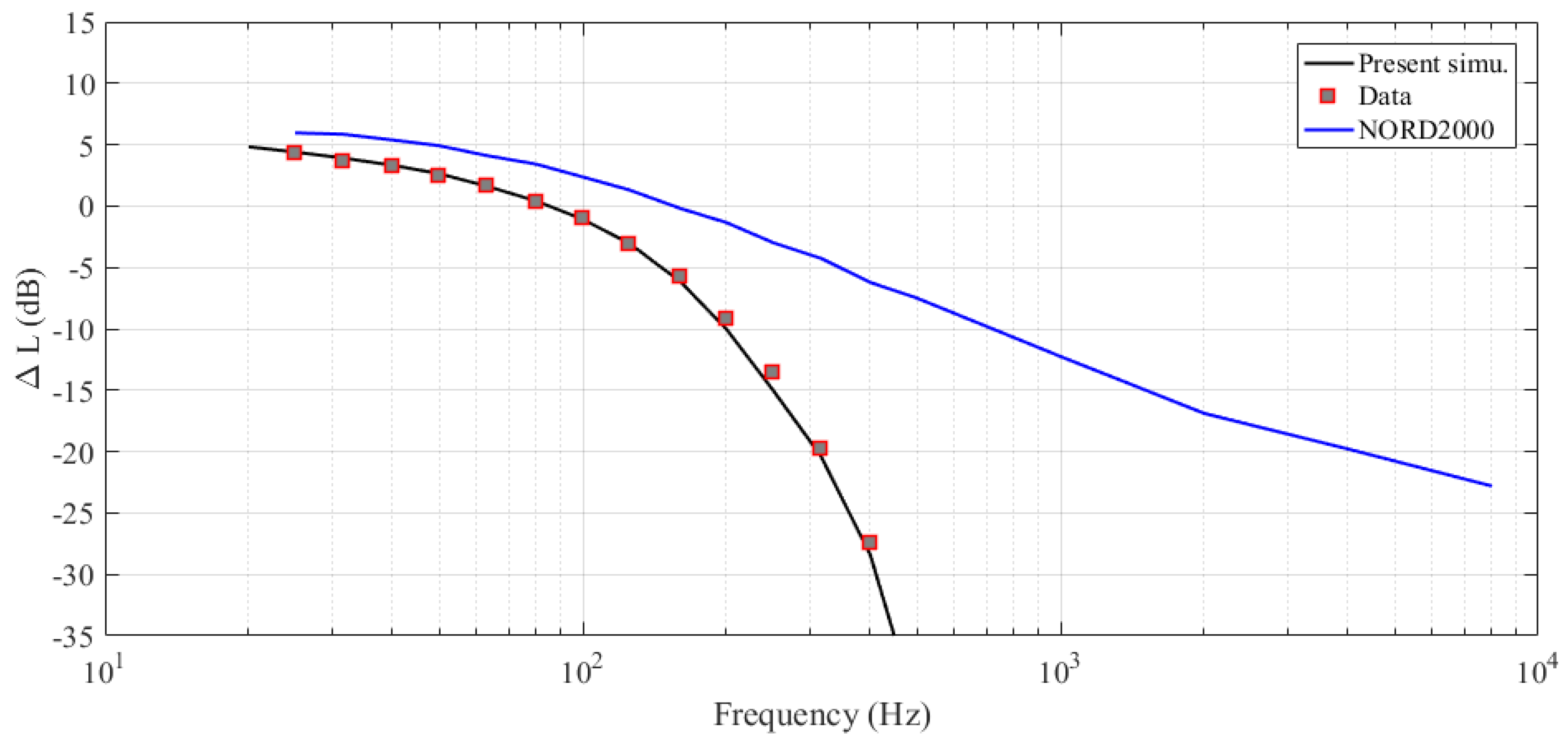
3.2. Validation of Long-Range Sound Propagations with a Positive Temperature Gradient

In this case, the terrain distance, source, and receiver locations remain the same, but the ground is an acoustically hard surface, meaning that the flow resistivity is close to infinity. The temperature gradient was measured as 0.0846 K/m. If a linear temperature variation is assumed, the temperature and sound speed profiles are easily computed using the following relations

$$T=\frac{\partial T}{\partial z}\cdot z+T_0$$

(13)

$$c=c_0\cdot \sqrt{T/T_0}$$

(14)

Such a temperature gradient leads to a downward sound propagation. As a result, the RSPL along the propagation direction will probably increase. In Figure 5, it is seen that there is a general increase of $\Delta L$ along the propagation path except near the source locations (x < 40 m). The $\Delta L$ values are gathered at x = 200 m distance and are depicted in Figure 6. It is found that the $\Delta L$ values are positive between 20 Hz and 5 kHz. The current prediction fits well with the reference data.

3.3. Validation of Long-Range Sound Propagations with Upward Refraction under Wind Condition

Similar as shown in the previous test case, the ground acoustic impedance is also infinity. However, an upward refraction case is considered which is caused by a moving atmosphere. The wind speed recorded at 10 m height above the ground is −4.165 m/s, and the surface roughness length is 0.1 m. In a moving medium, the sound speed can be computed using the equation below

$$c_{eff}\left(\mathrm{z}\right)=c_0+b\ln \left(\frac{z}{z_0}+1\right)$$

(15)

where $c_{eff}$ is the profile of effective sound speed along the vertical direction, $c_0$ = 340 m/s is the sound speed and $z_0$ = 0.1 m is the roughness height. Knowing the wind speed at 10 m height and the roughness length, it is easy to show that $b\approx -1$. Such a sound speed profile represents a slightly upward atmospheric refraction. In Figure 7, except at very low frequencies, the RSPL decays very fast along the propagation path. Figure 8 shows a very good agreement with the reference data which indicates the capability of the current method to handle noise propagations through moving media.

3.4. Coupled Flow and Noise Simulations for a Wind Turbine Array

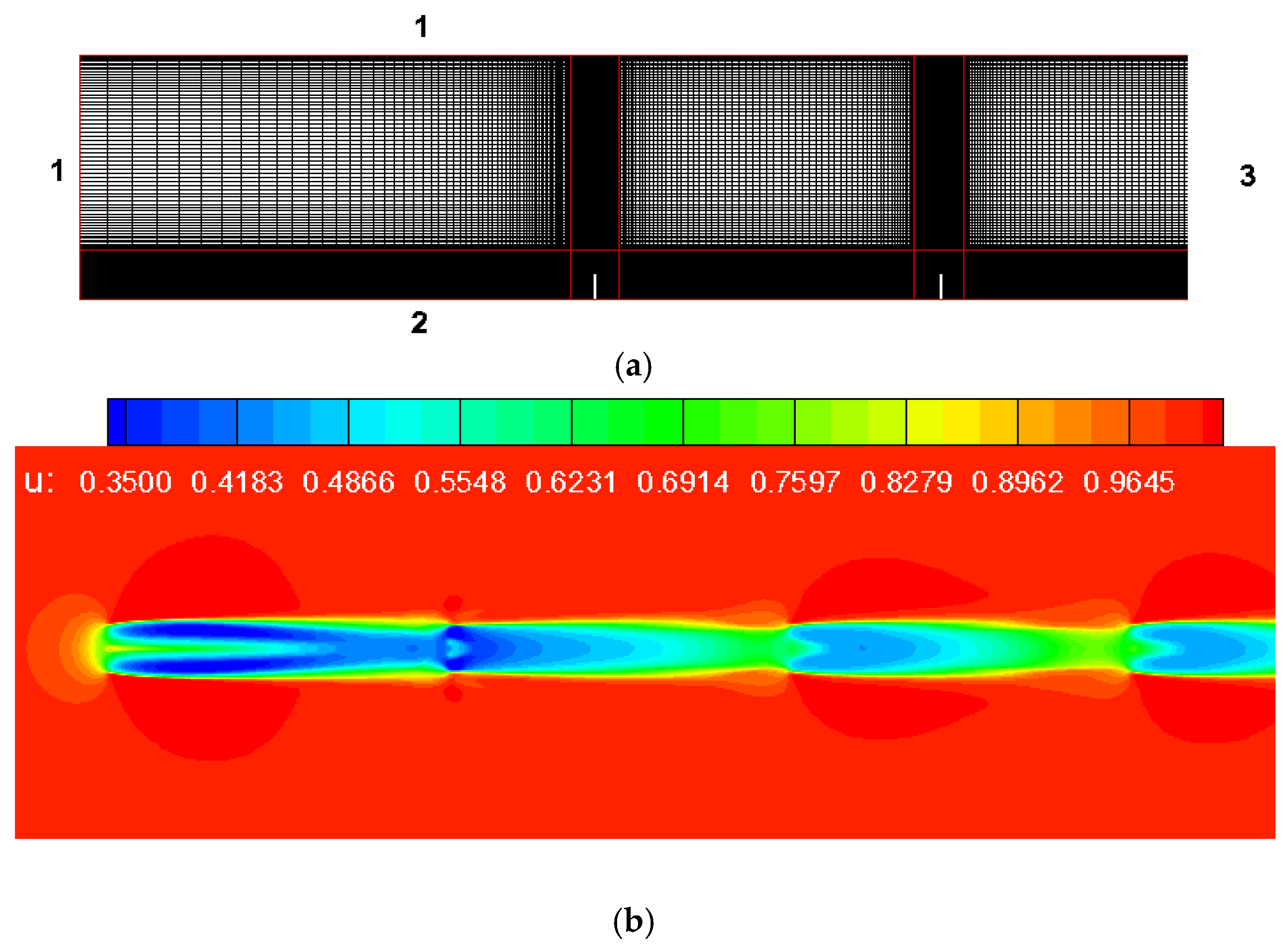
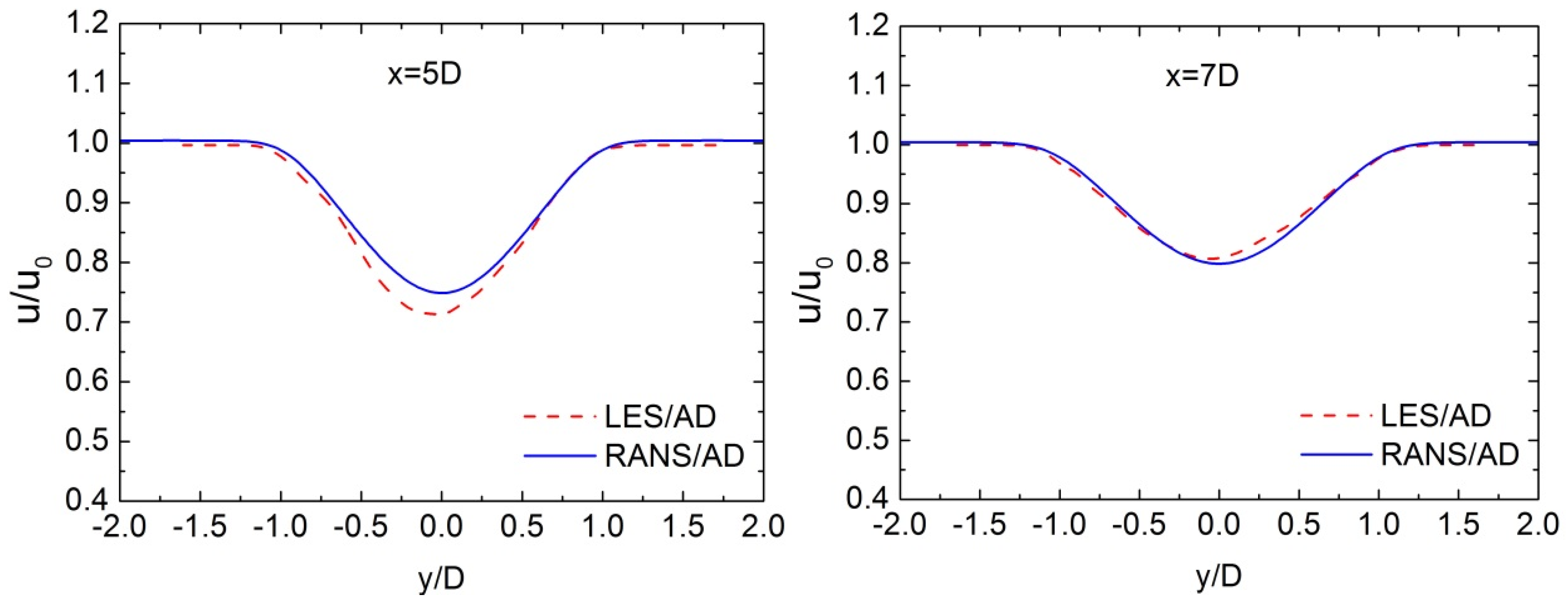
3.4.1. Wake Modeling of a Wind Turbine Cluster

Wind turbine flow are simulated for a Vestas wind turbine called NM80. The AOA and the relative velocity at all blade elements from RANS/AD simulations are inputted to the BPM model. The AD solver is much more efficient because it represents the rotor by volume force term rather than the dense body-fitted-mesh around blade surface. The flow computations are carried out with the in-house developed flow solver [24,25,26] which is an incompressible flow solver.

The grid for AD simulation and a typical flowfield with multi-wake structures are depicted in Figure 9. In Figure 9a, two wind turbines, depicted with thick white lines, are used for demonstration. The inflow boundary is applied on the left and top domain edge (numbered as 1 in Figure 9), the axisymmetric boundary on bottom edge (numbered as 2) and outflow boundary on the right edge (numbered as 3). The computational domain consists of the several blocks whose number is the same as that of wind turbines to be investigated. Each block contains grid points of 64 × 64. Using this approach, multi-wake flowfield can be efficiently modelled. A typical horizontal velocity contour plot is shown in Figure 9b.

To show the model accuracy, in Figure 10, some results from the current simulations using RANS turbulence model are compared with the LES results under same flow conditions [27,28]. On the modeling of wind turbine wake, many studies can be found [29,30,31]. In the present study, it is not of our primary interest to go into more details on this topic. Some more details of the AD modeling approach and cross comparisons can be found from our previous works [32,33,34].

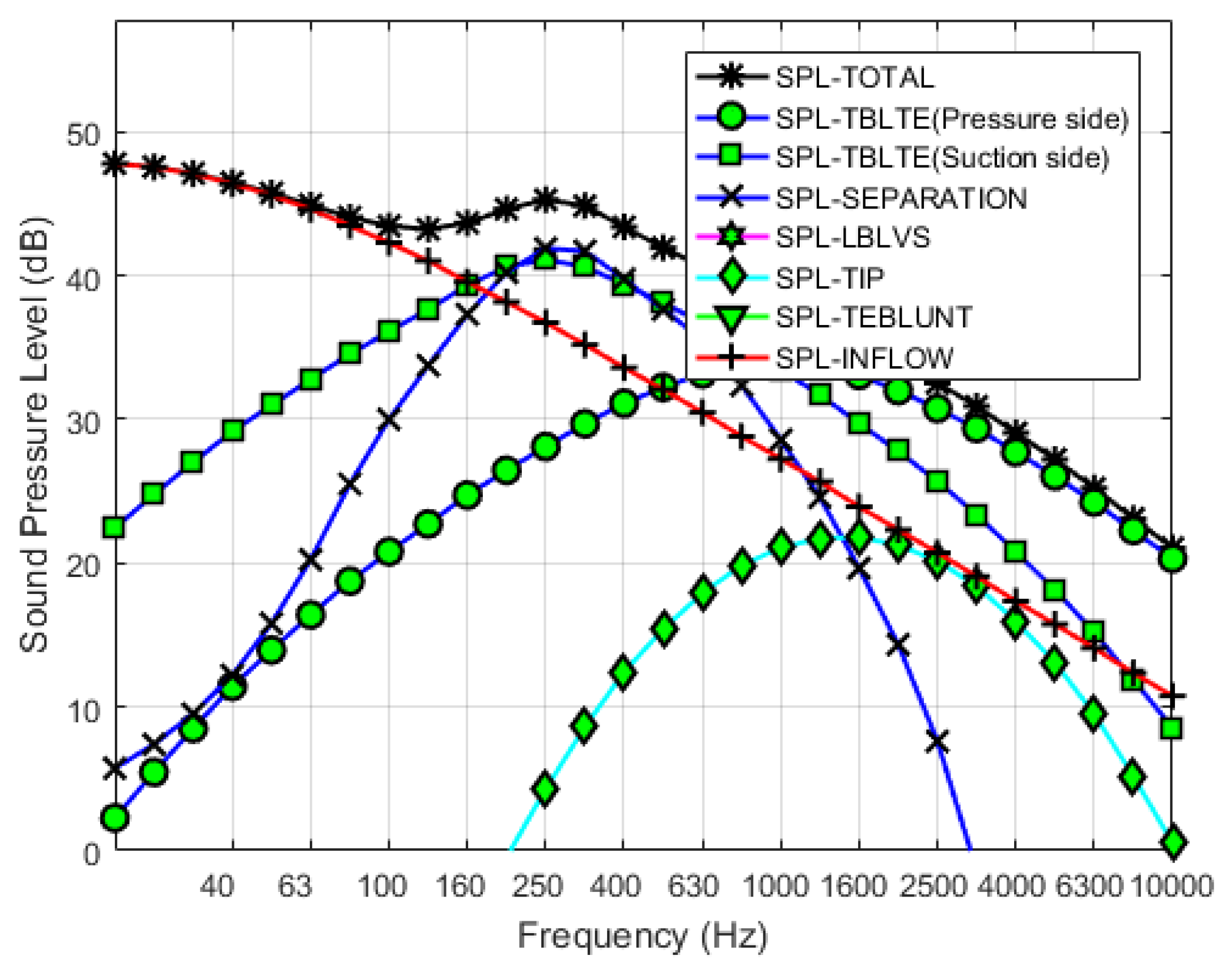
3.4.2. Modeling of the Wind Turbine ANSource

As is shown in the above AD simulation, every wind turbine has different inflow conditions because some wind turbines are in the wake of another, which leads to different ANSources. The simulation were conducted for a free-stream wind velocity of 8 m/s. For a receiver at 120 m far away, the detailed noise spectra solely from the first upstream wind turbine are shown in Figure 11. The noise spectra for other downstream wind turbines will be shown in the later sections. As shown in the figure, the total SPL spectrum is name as SPL-TOTAL which is logarithmically summed from several noise mechanisms. These noise mechanisms include: noise from blade tip (SPL-TIP); from trailing edge bluntness (SPL-TEBLUNT); from the shedding of laminar boundary layer vortex (SPL-LBLVS); from flow separation (SPL-SEPARATION); from turbulent boundary layer trailing edge (SPL-TBLTE); from turbulent inflow (SPL-INFLOW) [14,15,16]. Later, the total noise spectrum will be applied into the noise propagation computations.

3.4.3. Sound Profiles Inside wind Turbine Wakes

Although the flow and the noise source are modelled without wind and temperature gradients, in reality the effective sound speed profile will be affected by wind and temperature profiles. It was shown that the combinations of wind speed and temperature gradient forms different types of sound speed profiles [35]. Three idealized initial sound profiles are considered in the following sound propagation simulations. In Figure 12a, a uniform sound speed at temperature of 15 °C is assumed at the left boundary. The wind turbines are separated with a normalized distance of seven rotor diameters. For example, the second wind turbine is located at x = 560 m and the third wind turbine is located at x = 1120 m. Inside the computational domain, the sound speed is superimposed with the wind turbine wake field. Similarly, Figure 12b,c represent downward and upward sound speed contours. These sound profiles merge with the wind turbine multi-wakes and show distinct characteristics. The sound profiles have significant effects on wind turbine noise propagation as shown in the next subsection.

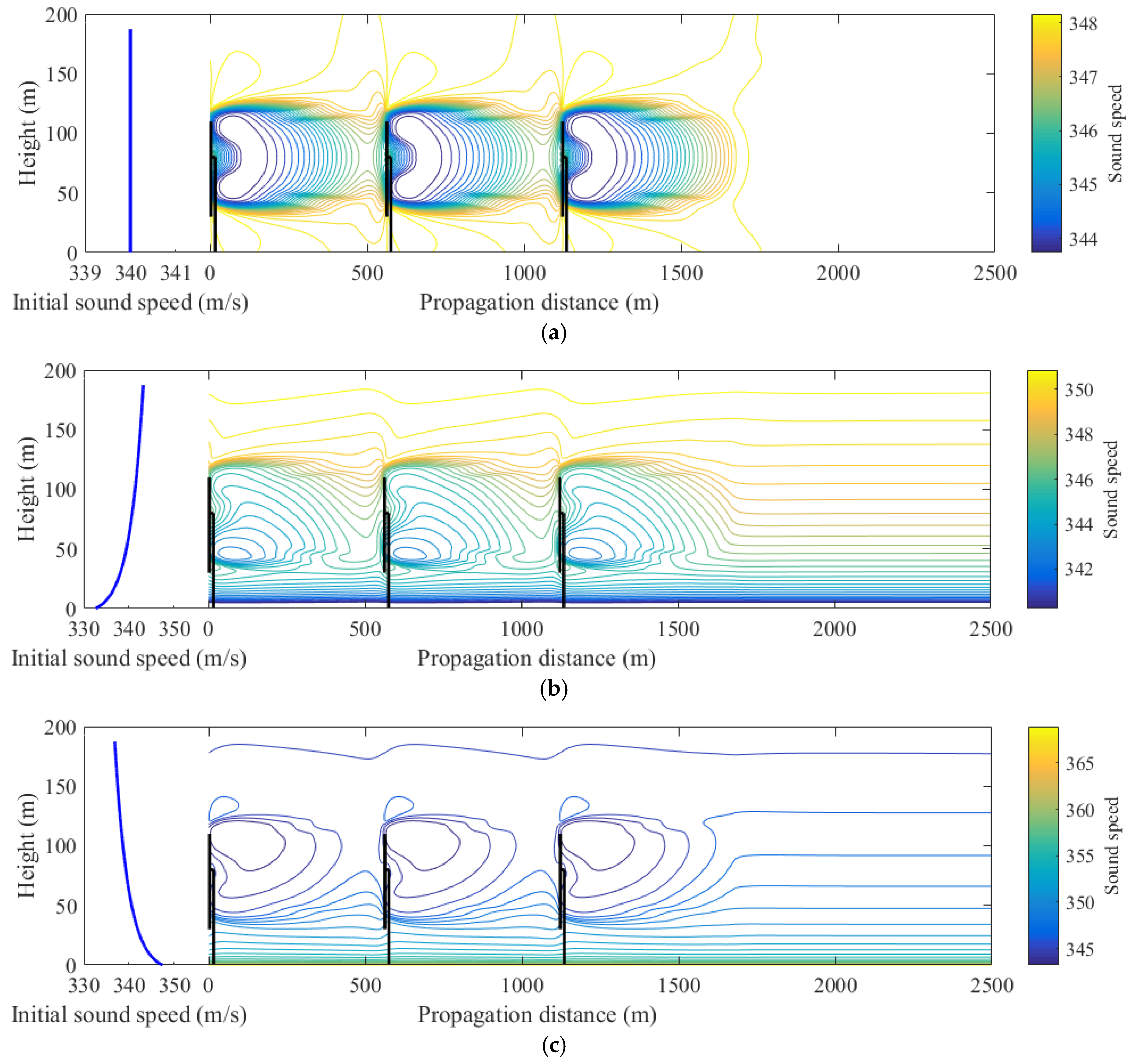
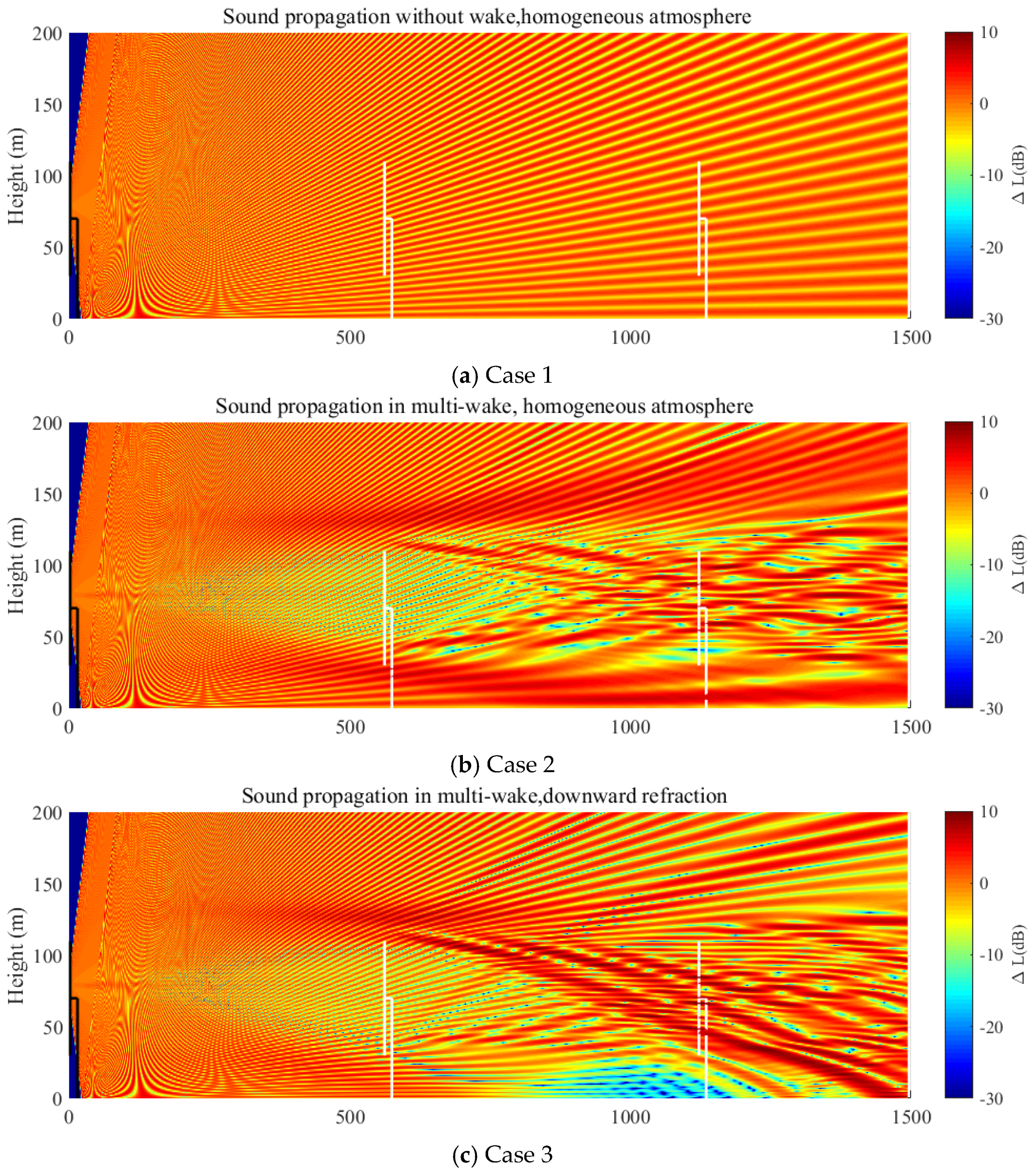
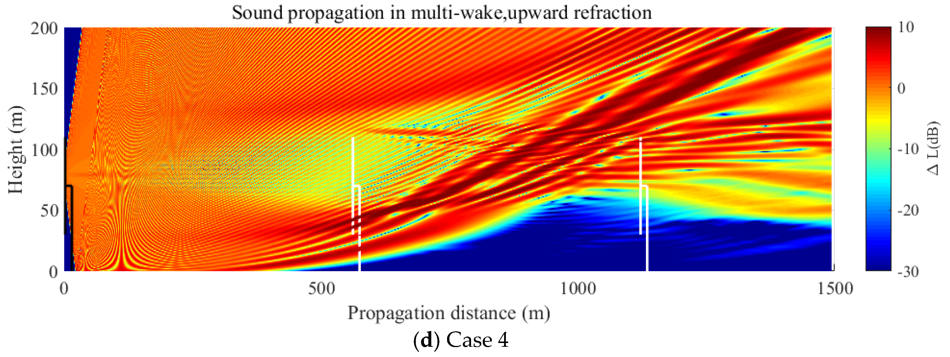
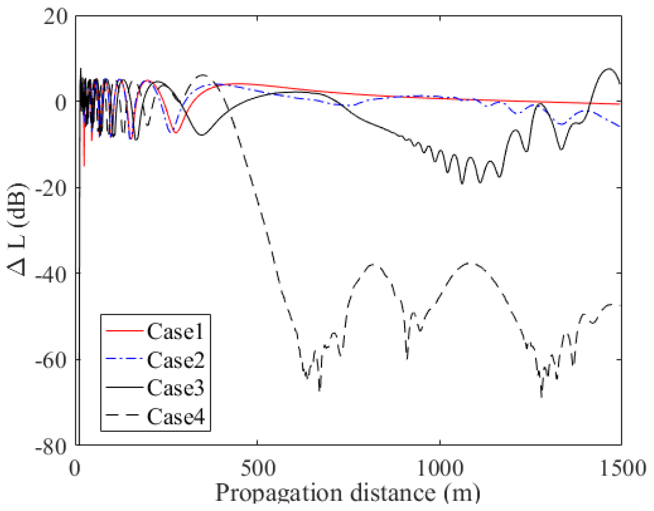
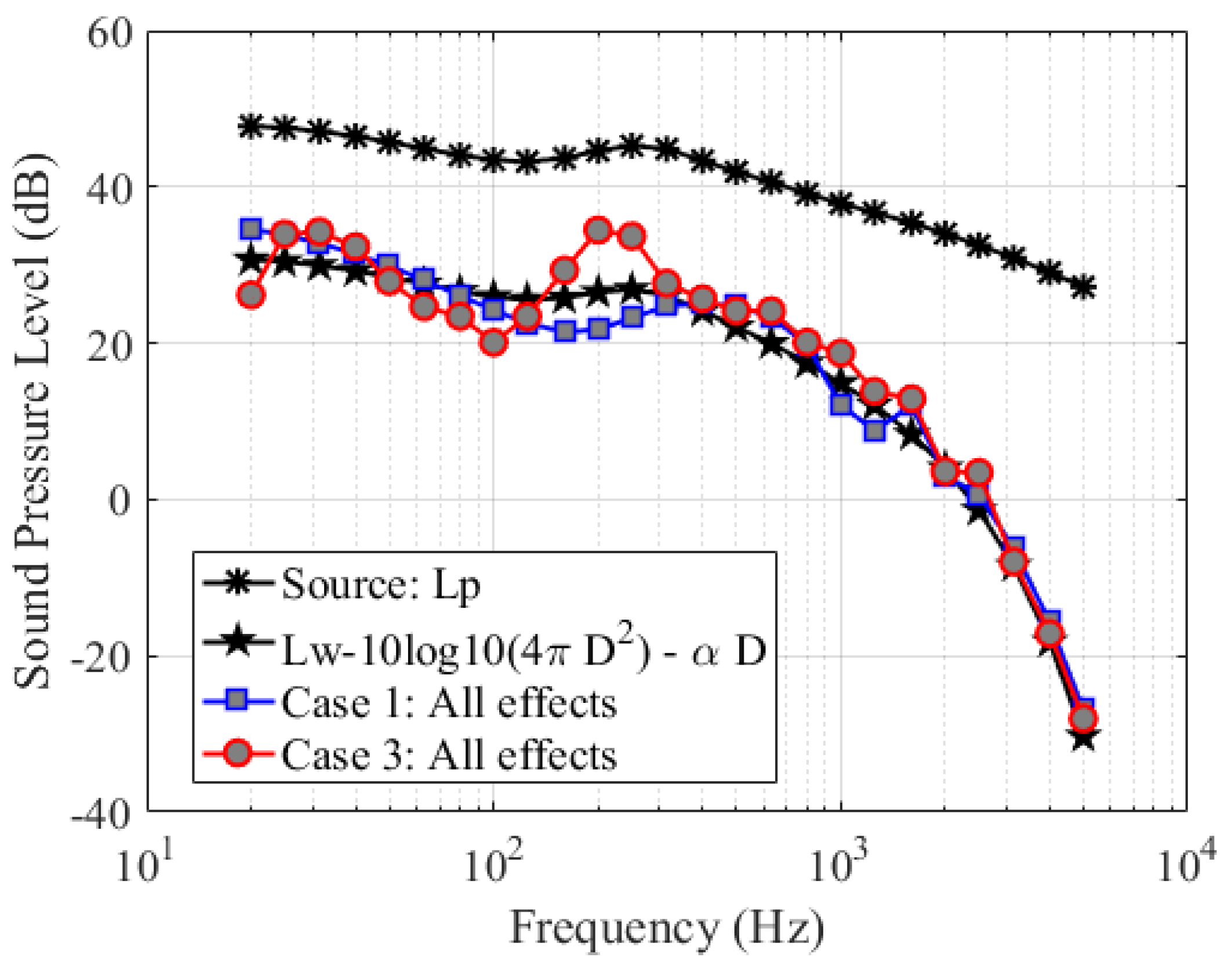
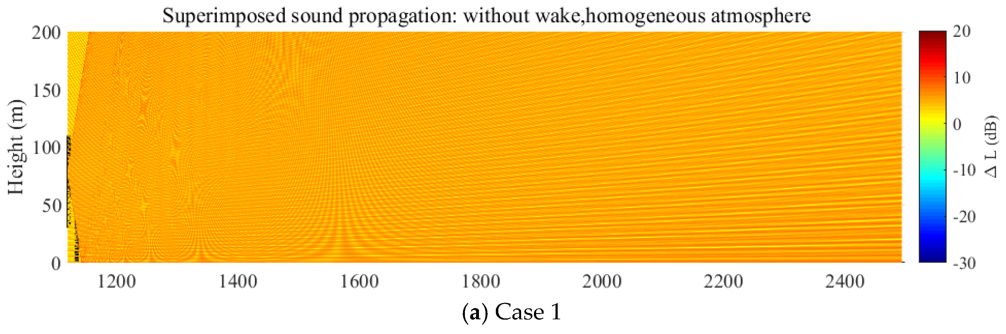
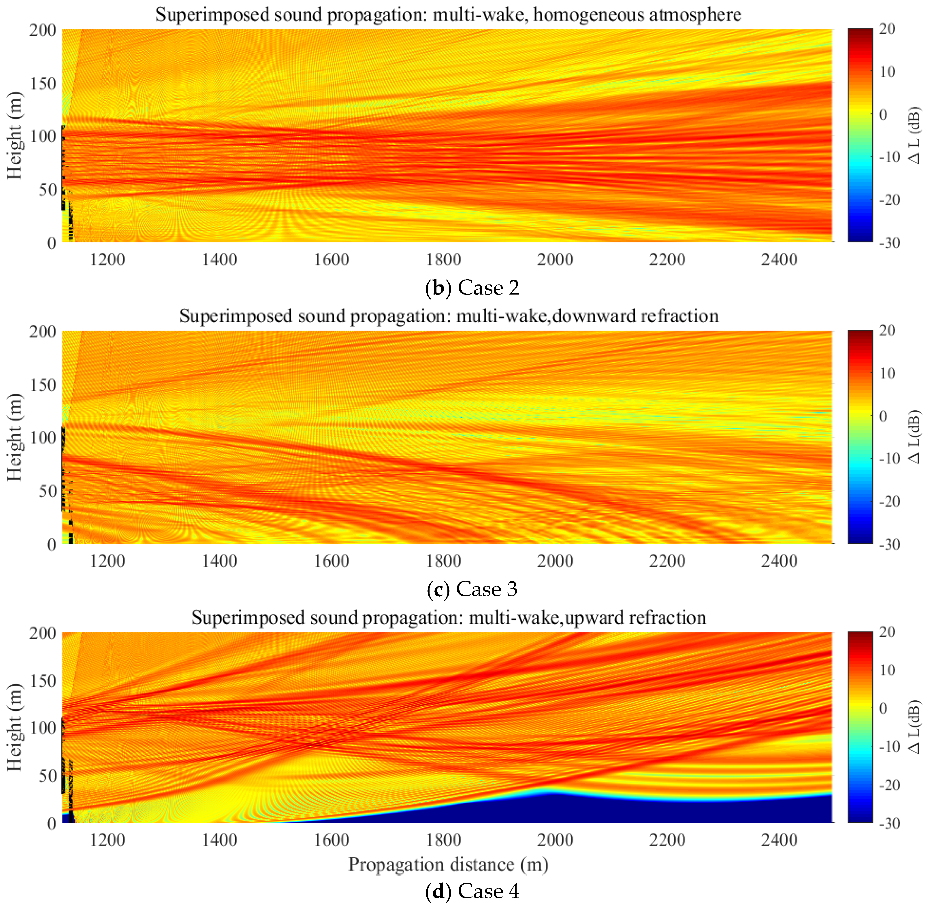
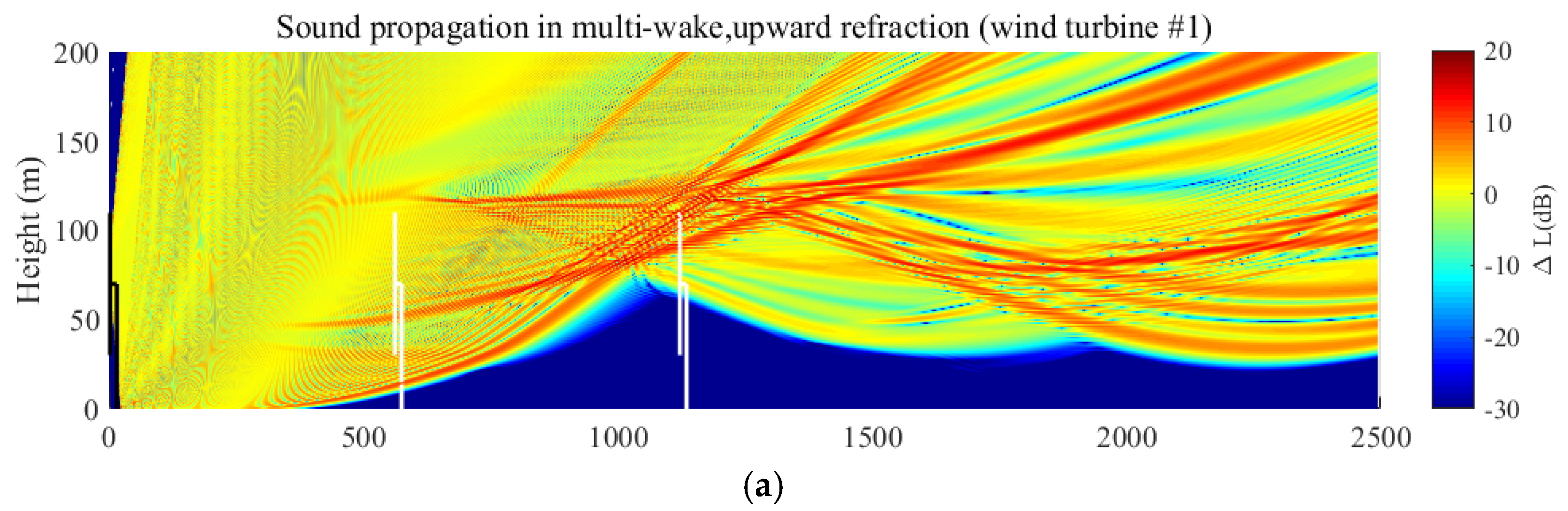
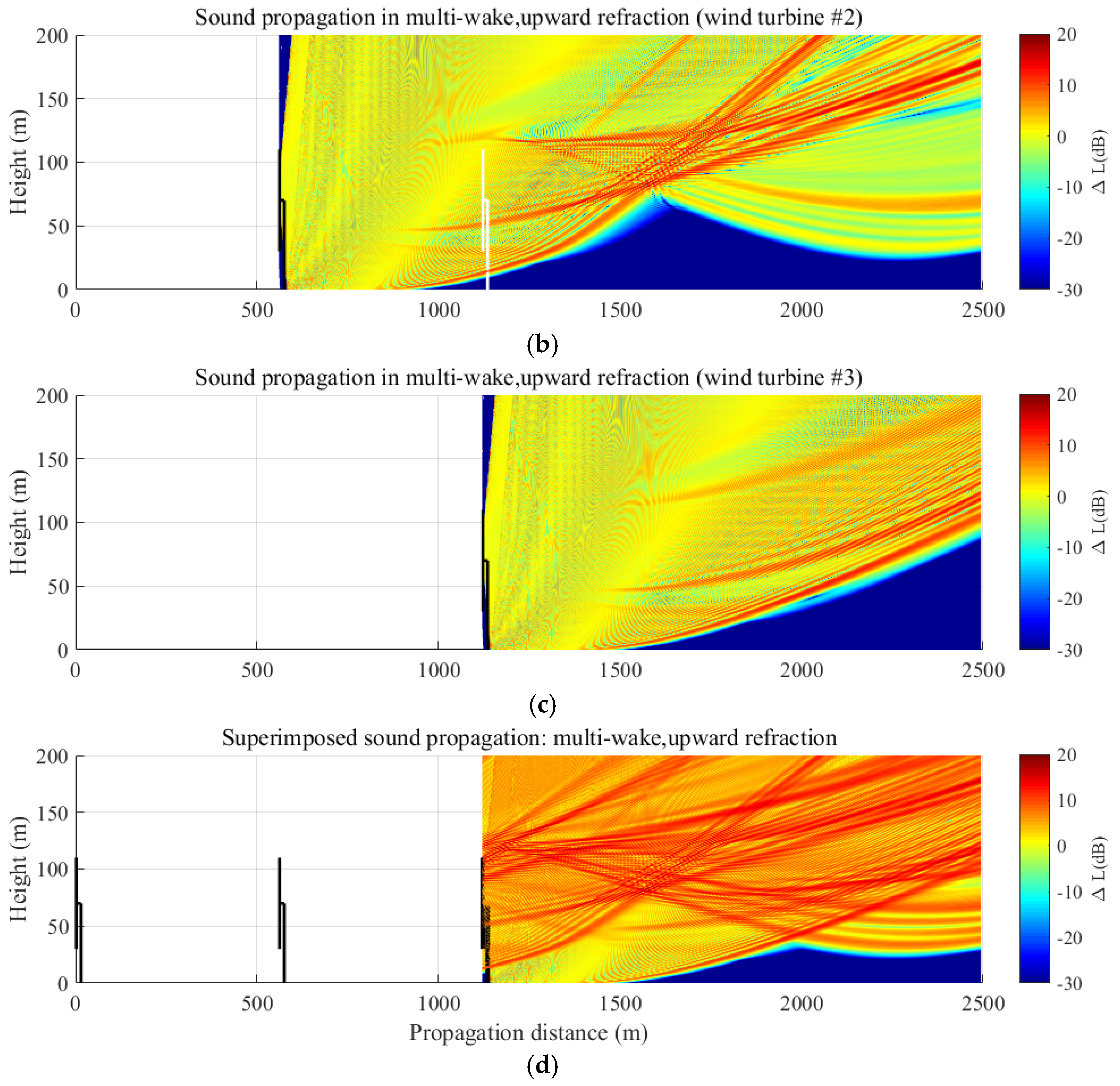
3.4.4. Wind Turbine ANPropagation across Multi-Wake

As shown in Figure 13, the RSPL or ∆L is simulated along 1500 m propagation distance, at f = 300 Hz and with the noise spectrum in Figure 11. The first wind turbine locates at x = 0 m, the second at 560 m and the third at 1120 m. The distance between each wind turbine are relative large. The wind turbine ANSource are placed at a height of 70 m. The ANSources from the second and third wind turbines, depicted as white lines, are not considered so as to focus on the propagation phenomenon through the wakes. In Figure 13, RSPL results are shown under several conditions: (1) Case 1, ANPropagation under homogeneous atmospheric condition, no wake effect; (2) Case 2, ANPropagation under homogeneous atmospheric condition, considering multi-wakes; (3) Case 3, ANPropagation under atmospheric condition of down-ward refraction, considering multi-wakes; (4) Case 4, ANPropagation under atmospheric condition of upward refraction, considering multi-wakes. It is shown that the wind turbine ANPropagation is clearly affected by the complicated flow environment. For the case without any wake effect shown in Figure 13a, the ANPropagation is mainly influenced by the reflection and absorption of ground. As is shown in Figure 13b, the contours of RSPL is more complicated than that of Figure 13a which distinctly shows the influences of wake. For atmospheric condition of downward refracting depicted in Figure 13c, the ‘noise pollution’ band also shows a downward reflecting behavior. Additionally, a low-noise zone, shown in blue, can be found near x = 1000 m. In Figure 13d, a much quieter situation is observed under an upward refraction condition. In such a case, the quiet zone is located between wind turbine #2 and #3. It should be emphasized that uniform inflow boundary condition is applied in the flowfield simulations of Figure 13c,d. However, the un-uniform or down/up-ward atmospheric conditions, which means atmospheric altitude-dependent variation of the sound speed, are used in the ANPropagation computations.

Manifesting the noise received by humans, the RSPL or ∆L at h = 2 m is extracted from Figure 13 and shown in Figure 14.The sound attenuation ∆L of Case 1 starts to vary linearly with the propagation distance at around x = 400 m, because the reflection effect becomes weaker after that. In contrast, the ∆L of Case 2, 3, and 4 vary obviously even after a long distance. In Cases 2 and 3, ∆L fluctuates over distance due to the wake effect and the strong downward refraction respectively. Whereas in Case 4, a more significant RSPL loss is shown which is caused by the upward refraction. It should be mentioned that the ∆L values might be quite different when the observer height changes. From this comparison, it can be concluded that ANPropagation can be greatly influenced by the environmental conditions. What is more, the change of SPL in the near downstream is much smaller than that at far downstream (x > 400 m), which shows the significance of long distance wind turbine noise predictions under complex atmospheric conditions. The near field (x < 400 m) simulations and measurements only belong to ANSource study which is not identical to the long-path ANPropagation.

Result shown in Figure 14 represents the ∆L solely due to propagation which is computed at a fixed frequency of f = 300 Hz. Repeating the calculation for many frequencies and extracting the data at a receiver 1500 m away and 2 m height, a full spectrum of ∆L will be obtained. Using Equation (12) and considering all the effects (including ∆L), the SPL at receiver’s location under Case 1 and Case 3 is gathered and shown in Figure 15. Besides, the spectrum of ANSource and at receiver’s location (without ∆L) are also depicted in Figure 15. In this work, the ANSource is considered in an 1/3-octave band from 20 Hz to 5000 Hz. Since a minimal eight grid points are needed to resolve a sound wave, the grid number for high-frequency simulations increases sharply if the same domain size is adopted. For instance, there is a 100-fold increase in the grid number for frequency of 3000 Hz compared with that of 300 Hz. To reduce the computational effort, frequencies above 5000 Hz are not considered here. Another reason is that the noise reduction due to air absorption, $-\alpha D$ in Equation (12), is much larger than the other factors at large frequency (f > 5000 Hz). The SPL at the source location is shown with black line with asterisk and labeled as ‘Source: Lp’ in Figure 15. The black lines with stars represent the SPL at receiver (2 m height at x = 1500 m) without considering the propagation loss ∆L in Equation (12). The blue line (Case 1) and red line (Case 3) consider all the factors, including geometric attenuation, air absorption and ∆L, in the long-path ANPropagation simulations. The big deviation between the two black lines demonstrates that the geometrical attenuation ($10{\log }_{10}4\pi D^2$) contributes most to the ANPropagation loss. The even larger reduction of noise, when f > 1000 Hz, means that air absorption has a larger effect at high frequencies. The differences between blue/red lines and the black line with stars implies the value of ∆L. The value of blue and red lines are larger than that of black line with stars, which means positive ∆L near low frequency (f = 30 Hz). However, Case 1 and Case 3 show opposite ∆L around f = 200 Hz which implies the influences of wake and downward refraction.

Similar as the previous simulations, the following study focuses on the noise propagation area between 1120 m and 2500 m, and a higher frequency f = 1000 Hz is selected. In this region, the three individual wind turbine noise sources propagate and superimpose on each other. In Figure 16a, the results cover the entire domain behind the last wind turbine. The solution differs from Figure 13a in the sense that it is the RSPL from all the three wind turbines. In Figure 16b, the uniform sound profile at the inlet boundary is affected by the multi-wake (see Figure 12a), such that the resulted RSPL is enhanced around wake center. With the prescribed sound profile of Figure 12b, the RSPL is refracted downwards, as shown in Figure 16c. Similarly, using the sound profile given in Figure 12c, the resultant sound propagation is refracted upwards, see Figure 16d.

Figure 17 better illustrates the superposition of the sound pressure propagates from each wind turbine, which is a decomposition of Figure 16d. In the first figure, noise is generated from wind turbine #1 and propagates through the wake flow. The other two wind turbines are depicted with white lines, which imply that they are currently excluded for noise propagation. In the next simulation, shown in Figure 17b, ANPropagation from wind turbine #2 is individually considered, which excluded noise propagation from wind turbine #1 and #3. Similarly, wind turbine #3 is then considered for ANPropagation, which does not take account of the two upstream wind turbine noise propagations. The total RSPL is the summation of sound pressure following the logarithmic sumation rule, which is shown in Figure 17d.

Figure 18 shows the RSPL or ∆L extracted from a line at 2 m high. The overall sound pressure variation for different cases is smaller as compared to the previous results shown in Figure 14. This is due to the mixing of three individually simulated propagation field. Among all the test cases, Case 3 can be regarded as the worst-case scenario. For example, around the distance of x = 1800 m, there is an obvious increase of SPL due the strong downward refraction at this region, which is also observed in Figure 16c at x = 1800 m.

Similar to the procedures previously mentioned for Figure 15, Figure 19a–c show the noise spectra from wind turbines #1, 2, and 3, respectively. The difference is that the three wind turbines are individually considered for its noise generation and propagation at the given frequencies (20 Hz–5000 Hz). Due to the presence of velocity deficit in the wake, the inflow conditions of the two downstream wind turbines are slightly different, and thus the ANSources of the three wind turbines are slightly different from each wind turbine. In each figure, the original ANSource is shown on top of the other noise spectra. Similar to the situations in Figure 15, geometrical attenuation plays an primary role in the large noise reduction for ANPropagation at f < 1000 Hz, and the noise absorption by air has a strong effect at f > 1000 Hz. As expected, Case 3 shows more distinct characteristics for the frequencies. In Figure 19, the receiver is fixed at x = 2500 m, z = 2 m, therefore the sound pressure is largely attenuated for wind turbine #1 due to the longest propagation distance. A similar behavior is seen for wind turbines #2 and #3, where the noise level is the highest for wind turbine #3 due to the shortest relative distance from source to receiver. Figure 19a–c also show that at different relative propagation distances 2500 m (#1), 1940 m (#2) and 1380 m (#3), the distribution of SPL maintains some similarity. The differences of these sound spectra come from the combined effect of wake flow and the propagation distance. Finally, the total noise received from the three wind turbines can be got through logarithmically adding the sound spectra from individual wind turbines. In Figure 19d, the sources Lp1, Lp2, and Lp3 represent the ANSource level of the three wind turbines. The major difference is seen at the middle frequency range, which is due to the different input velocity data obtained from flow simulation. Case 1 and Case 3 all show that the most significant influence comes from wind turbine #3, which is not a surprise. To highlight more detailed difference in the noise spectra, a few typical values are compared in

Table 1. Comparisons of SPL at some selected frequencies

	Case 3 (Figure 19c)	Case 3 (Figure 19d)	${\mathit{L}}_{\mathit{w}}-10{\mathbf{log}}_{10}4\mathit{\pi }{\mathit{D}}^2-\mathit{\alpha }\mathit{D}$ (Figure 19d)
20 (Hz)	34.64 dB	37.92 dB	33.89 dB
100 (Hz)	12.61 dB	15.05 dB	28.53 dB
250 (Hz)	26.25 dB	28.33 dB	27.57 dB
1000 (Hz)	17.10 dB	17.99 dB	18.00 dB

. At f = 20 Hz, the summated SPL from three turbines (Case 3) is 37.92 dB which is 3 dB higher than that from wind turbine #3 (Case 3). This difference becomes smaller when frequency increases. This implies that the low frequency noise generated from the far upstream wind turbines still plays an important role. On the other hand, if a simple sound propagation algorithm is applied, such as shown in the last column of Table 1, a large error is observed in a frequency range below 1000 Hz. It indicates that the high frequency noise will be heavily attenuated over long propagation distance except in special cases such as sound propagation over water (hard surface), stronger downward refraction under special climate conditions.

Finally, it is interesting to predict the noise spectra at different receivers. The receiver height is again fixed at z = 2 m, and the horizontal distances measured from wind turbine #1 are: x = [1620, 1820, 2020, 2220, 2420] m. The noise spectra are shown in Figure 20 and marked with different colors. The general trend is that the noise level decreases as observer distance increases. However, it does not always hold true at some distances and frequencies. For example, at x = 1820 m (22.75D), except at low frequencies, increase of noise level is observed as compared to the x = 1620 m case. The simulations show that the low frequency noise might be the major wind turbine noise source in the farfield. Since the spectra are obtained in farfield, the overall SPLs are quite low. According to the wind turbine noise regulations in many countries (such as 45 dB), the calculated noise evidently fulfill the limit. From the results, it is seen that SPLs over 1000 Hz is below 20 dB. For future studies, it is indicated that more focus should be paid on long-path ANPropagation at low frequencies.

4. Conclusions

Combing the flowfield aerodynamic simulation and the aeroacoustics computation of multi-wind turbines is the focus of this paper. To achieve this objective, ANSource modeling, flow simulation and ANPropagation are individually described and then integrated. The numerical computations are carried out using the in-house developed tool EllipSys. The ANSource modeling and ANPropagation modeling are implemented in the platform of EllipSys. The steady CFD simulations are performed to obtain the flowfield with a relatively efficient 2D-AD solver. The ANSource of wind turbine is calculated using the flowfield information from CFD computations. Then the ANPropagation is simulated which needs the data from both CFD simulations and ANSource computations. Results from different case studies show that a long-path ANPropagation are greatly influenced by different flow conditions, atmosphere conditions and wake condition. An overall trend is that the ANSource from wind turbines is broadband, but the received noise level at long travelling distances from multi-wind turbines is complicated. The noise spectra show that the low frequency noise from a wind turbine cluster might be an important issue to be further investigated. It has been shown in the results that at a distance over 1 km (about 12 rotor diameter), the high frequency components are largely attenuated, say at f > 1000 Hz. In a large wind farm with superimposition of noise sources from multi-wind turbines, the computational load will be heavy if high frequency noise is simulated. The ray theory, as compared in Section 3.1, Section 3.2 and Section 3.3, is a high-frequency approach therefore the low frequency solutions are not very accurate if strong refraction and diffraction are represented. The present numerical approach has same accuracy over all frequency range. However, to solve high frequency ANPropagation, higher grid density is required, thus increasing computational time. Fortunately, results presented in Figure 18 and Figure 19 indicate that it is the low frequency noise components that contribute to the long range wind turbine ANPropagation. The receiver distances shown in Figure 19 ranges from 20 to 30 rotor diameters. It is clear that at such a large distance, attenuation of low frequency noise is still not significant.

References

1. Glauert, H. Airplane Propellers. Aerodynamic Theory; Springer: Berlin/Heidelberg, Germany, 1935; pp. 169–360. [Google Scholar]
2. Sun, Z.Y.; Chen, J.; Shen, W.Z.; Zhu, W.J. Improved blade element momentum theory for wind turbine aerodynamic computations. Renew. Energy 2016, 96, 824–831. [Google Scholar] [CrossRef]
3. Sørensen, J.N.; Shen, W.Z. Numerical Modeling of Wind Turbine Wakes. J. Fluids Eng. 2002, 124, 393. [Google Scholar] [CrossRef]
4. Sørensen, J.N.; Shen, W.Z.; Munduate, X. Analysis of wake states by a full-field actuator disc model. Wind Energy 1998, 1, 73–88. [Google Scholar] [CrossRef]
5. Lighthill, M.J. On Sound Generated Aerodynamically. I. General Theory. Proc. R. Soc. Lond. 1952, 211, 564–587. [Google Scholar] [CrossRef]
6. Curle, N. The Influence of Solid Boundaries upon Aerodynamic Sound. Proc. R. Soc. Lond. 1955, 231, 505–514. [Google Scholar] [CrossRef]
7. Williams, J.E.; Hall, L.H. Aerodynamic sound generation by turbulent flow in the vicinity of a scattering half plane. J. Fluid Mech. 2006, 40, 657–670. [Google Scholar] [CrossRef]
8. Hardin, J.C.; Pope, D.S. An acoustic/viscous splitting technique for computational aeroacoustics. Theor. Comput. Fluid Dyn. 1994, 6, 323–340. [Google Scholar] [CrossRef]
9. Zhu, W.J.; Shen, W.Z.; Sørensen, J.N. High-order numerical simulations of flow-induced noise. Int. J. Numer. Methods Fluids 2011, 66, 17–37. [Google Scholar] [CrossRef]
10. Zhu, W.J.; Shen, W.Z.; Barlas, E.; Bertagnolio, F.; Sørensen, J.N. Wind turbine noise generation and propagation modeling at DTU Wind Energy: A review. Renew. Sustain. Energy Rev. 2018, 88, 133–150. [Google Scholar] [CrossRef]
11. Salomons, E.M. Computational Atmospheric Acoustics; Springer Science & Business Media: Dordrecht, The Netherlands, 2001; ISBN 978-1-4020-0390-5. [Google Scholar]
12. Ostashev, V.E.; Wilson, D.K. Acoustics in Moving Inhomogeneous Media. J. Acoust. Soc. Am. 1999, 105, 2067. [Google Scholar] [CrossRef]
13. Blancbenon, P.; Dallois, L.; Juvé, D. Long Range Sound Propagation in a Turbulent Atmosphere Within the Parabolic Approximation. Acta Acust. United Acust. 2001, 87, 659–669. [Google Scholar] [CrossRef]
14. Brooks, T.F.; Pope, D.S.; Marcolini, M.A. Airfoil Self-Noise and Prediction; National Aeronautics and Space Administration: Washington, DC, USA, 1989.
15. Zhu, W.J.; Heilskov, N.; Shen, W.Z.; Sørensen, J.N. Modeling of Aerodynamically Generated Noise From Wind Turbines. J. Sol. Energy Eng. 2005, 127, 517–528. [Google Scholar] [CrossRef]
16. Lau, A.S.H.; Kim, J.W.; Hurault, J.; Vronsky, T. A study on the prediction of aerofoil trailing-edge noise for wind-turbine applications. Wind Energy 2017, 20, 233–252. [Google Scholar] [CrossRef]
17. Lee, S.; Lee, D.; Honhoff, S. Prediction of far-field wind turbine noise propagation with parabolic equation. J. Acoust. Soc. Am. 2016, 140, 767–778. [Google Scholar] [CrossRef] [PubMed] [Green Version]
18. Heimann, D.; Käsler, Y.; Gross, G. The wake of a wind turbine and its influence on sound propagation. Meteorol. Z. 2011, 20, 449–460. [Google Scholar] [CrossRef]
19. Barlas, E.; Zhu, W.J.; Shen, W.Z.; Kelly, M.; Andersen, S.J. Effects of wind turbine wake on atmospheric sound propagation. Appl. Acoust. 2017, 122, 51–61. [Google Scholar] [CrossRef]
20. Barlas, E.; Zhu, W.J.; Shen, W.Z.; Dag, K.O.; Moriarty, P. Consistent modelling of wind turbine noise propagation from source to receiver. J. Acoust. Soc. Am. 2017, 142, 3297. [Google Scholar] [CrossRef]
21. Delany, M.E.; Bazley, E.N. Acoustical properties of fibrous absorbent materials. J. Acoust. Soc. Am. 2005, 48, 105–116. [Google Scholar] [CrossRef]
22. Jónsson, G.B.; Jacobsen, F. A Comparison of Two Engineering Models for Outdoor Sound Propagation: Harmonoise and Nord2000. Acta Acust. United Acust. 2008, 94, 282–289. [Google Scholar] [CrossRef]
23. Plovsing, B.; Kragh, J. Nord2000-Comprehensive Outdoor Sound Propagation Model. Part 2: Propagation in an Atmosphere with Refraction; Delta Acoustics & Vibration Report; DELTA: Copenhagen, Denmark, 2006. [Google Scholar]
24. Mikkelsen, R. Actuator Disc Methods Applied to Wind Turbines. Ph.D. Thesis, Technical University of Denmark, Copenhagen, Denmark, 2003. [Google Scholar]
25. Michelsen, J.A. Basis3D-A Platform for Development of Multiblock PDE Solvers; Technical Report; University of Denmark: Copenhagen, Denmark, 1992. [Google Scholar]
26. Sørensen, N. General Purpose Flow Solver Applied over Hills; Technical Report; Risø National Laboratory: Roskilde, Denmark, 1995. [Google Scholar]
27. Tian, L.L.; Zhu, W.J.; Shen, W.Z.; Zhao, N.; Shen, Z.W. Development and validation of a new two-dimensional wake model for wind turbine wakes. J. Wind Eng. Ind. Aerodyn. 2015, 137, 90–99. [Google Scholar] [CrossRef] [Green Version]
28. Wu, Y.T.; Porté-Agel, F. Modeling turbine wakes and power losses within a wind farm using LES: An application to the Horns Rev offshore wind farm. Renew. Energy 2015, 75, 945–955. [Google Scholar] [CrossRef]
29. Sarmast, S.; Segalini, A.; Mikkelsen, R.F.; Ivanell, S. Comparison of the near-wake between actuator-line simulations and a simplified vortex model of a horizontal-axis wind turbine. Wind Energy 2016, 19, 471–481. [Google Scholar] [CrossRef]
30. Troldborg, N.; Sørensen, J.N.; Mikkelsen, R. Numerical simulations of wake characteristics of a wind turbine in uniform inflow. Wind Energy 2010, 13, 86–99. [Google Scholar] [CrossRef]
31. Troldborg, N.; Zahle, F.; Réthoré, P.E.; Sørensen, N.N. Comparison of wind turbine wake properties in non-sheared inflow predicted by different computational fluid dynamics rotor models. Wind Energy 2015, 18, 1239–1250. [Google Scholar] [CrossRef]
32. Tian, L.L.; Zhu, W.J.; Shen, W.Z.; Sørensen, J.N.; Zhao, N. Investigation of modified AD/RANS models for wind turbine wake predictions in large wind farm. J. Phys. 2014. [Google Scholar] [CrossRef]
33. Tian, L.L.; Zhu, W.J.; Shen, W.Z.; Song, Y.L.; Zhao, N. Prediction of multi-wake problems using an improved Jensen wake model. Renew. Energy 2017, 102, 457–469. [Google Scholar] [CrossRef]
34. Zhu, W.J.; Shen, W.Z.; Sørensen, J.N.; Yang, H. Verification of a novel innovative blade root design for wind turbines using a hybrid numerical method. Energy 2017, 141, 1661–1670. [Google Scholar] [CrossRef]
35. Wilson, D.K.; Pettit, C.L.; Ostashev, V.E. Sound propagation in the atmospheric boundary layer. Acoust. Today 2015, 11, 44–53. [Google Scholar] [CrossRef]
Figure 1. Schematic diagram of relations between the developed solvers.
Applsci 09 00100 g001
Figure 2. Demonstration of grids in the plane of propagation utilized in the simulations.
Applsci 09 00100 g002
Figure 3. Sound transmission loss over 200 m at various frequencies (soft ground).
Applsci 09 00100 g003
Figure 4. Comparisons of the RSPL in 1/3-octave bands.
Applsci 09 00100 g004
Figure 5. Sound transmission loss over 200 m at various frequencies (rigid ground and downward refraction).
Applsci 09 00100 g005
Figure 6. Comparisons of the RSPL in 1/3-octave bands at a distance of 200 m.
Applsci 09 00100 g006
Figure 7. Sound transmission loss over 200 m at various frequencies (rigid ground and upward refraction).
Applsci 09 00100 g007
Figure 8. Comparisons of the RSPL in 1/3-octave bands.
Applsci 09 00100 g008
Figure 9. (a) Mesh topology; (b) stream-wise flow with multi-wakes.
Applsci 09 00100 g009
Figure 10. Comparisons of the normalized wake velocity from LES and RANS simulations, for down-stream locations of 5D and 7D after a single wind turbine.
Applsci 09 00100 g010
Figure 11. Aerodynamic noise source spectra of a single wind turbine.
Applsci 09 00100 g011
Figure 12. Initial sound speed profiles at upstream and effective sound speed contours in the wake flow. (a) Uniform initial sound profile transmitted into wake; (b) upward refraction sound profile transmitted into wake; (c) downward refraction sound profile transmitted into wake.
Applsci 09 00100 g012
Figure 13. ANPropagation from the first ANSource: (a) Case 1, homogeneous atmospheric condition, no wake effect; (b) Case 2, homogeneous atmospheric condition with multi-wakes; (c) Case 3, downward refraction and multi-wakes; (d) Case 4, upward refraction and multi-wakes.
Applsci 09 00100 g013aApplsci 09 00100 g013b
Figure 14. The RSPL at 2 m height extracted from four cases of Figure 13.
Applsci 09 00100 g014
Figure 15. SPL of wind turbine #1 (Source: Lp) received at 1500 m distance (2 m height): with geometric attenuation and air absorption, Case 1 and Case 3 with all propagation effects.
Applsci 09 00100 g015
Figure 16. ANPropagation from all ANSources: (a) Case 1, homogeneous atmospheric condition, no wake effect; (b) Case 2, homogeneous atmospheric condition with multi-wakes; (c) Case 3, downward refraction and multi-wakes; (d) Case 4, upward refraction and multi-wakes.
Applsci 09 00100 g016aApplsci 09 00100 g016b
Figure 17. RSPL simulated at f = 1000 Hz and b = −3: (a) ANPropagation by wind turbine #1 downstream of the wakes of wind turbines # 1, 2, 3; (b) ANPropagation by wind turbine #2 downstream of the wakes of wind turbines #2, 3; (c) ANPropagation by wind turbine #3 downstream of the wakes of wind turbine #3; (d) superimposed RSPL from all wind turbines #1, 2, 3.
Applsci 09 00100 g017aApplsci 09 00100 g017b
Figure 18. The RSPL at 2 m height extracted from four cases of Figure 16.
Applsci 09 00100 g018
Figure 19. Receiver is fixed at x = 2500 m away from wind turbine #1, and the receiver height is 2 m. (a) SPL from wind turbine #1 (Source: Lp) to the receiver; (b) SPL from wind turbine #2 (Source: Lp) to the receiver; (c) SPL from wind turbine #3 (Source: Lp) to the receiver; (d) Total SPL from wind turbines #1, 2, 3 (Source: Lp1, Lp2, Lp3).
Applsci 09 00100 g019
Figure 20. Total SPL from wind turbines #1, 2, 3 received at various distance.
Applsci 09 00100 g020