Condition Prediction of Existing Concrete Bridges as a Combination of Visual Inspection and Analytical Models of Deterioration

Abstract

In most state-of-the-art Bridge Management Systems, structural condition is predicted by a homogeneous Markov chain model that uses condition ratings assigned during visual inspections. Although generally accepted, such an approach exhibits certain shortcomings, one of which is not considering the nature of actual physical phenomena that cause deterioration. To overcome this shortcoming, this article presents a framework that combines both information on condition ratings through the semi-Markov process and knowledge of bridge properties using analytical deterioration models. In this manner, and contrary to current practice, not only are the results of visual inspection taken into account, but also information such as environmental loading, as well as material and structural properties. The presented framework was implemented in the case study bridge, in which the deterioration caused by carbonation-induced corrosion was studied. Along with the implementation in the case study, the article contained a detailed overview of the subject of carbonation-induced corrosion and emphasized issues that require additional research in order to develop the framework into a comprehensive and fully applicable tool for condition prediction. Accounting for its adaptability to other material types and deterioration processes and its consideration of the historic deterioration path, the framework presents a suitable alternative to frameworks presently implemented for condition prediction.

1. Introduction

Bridges are vital elements of roadway and railway transportation infrastructure and they require timely decision-making to schedule Maintenance, Repair and Rehabilitation (MR&R) activities. To support the decision-making process, an increasing number of computer-aided Bridge Management Systems (BMSs) have been developed over the past two decades [1]. The main goal of the BMS is to establish an optimal operation strategy as a compromise between technical and social factors, such as maximization of network performance, minimization of life-cycle costs, and minimization of the probability of failure [2]. To establish such a strategy, it is essential to comprehend the long-term performance of a bridge, taking into account possible deterioration [3,4].

For the prediction of the long-term performance of a bridge, most BMS software today uses statistical models based on condition ratings of bridge components or of an overall bridge, where the homogeneous Markov chain model is the most frequent [5]. In cases where condition prediction is purely based on condition ratings, the knowledge of how materials and elements are affected by the surrounding environment is not being fully employed [6]. Hence, implementing analytical deterioration models in BMSs, such as, e.g., the one describing the carbonation-induced corrosion, presents a suitable complement to current state. Moreover, significant research in the area of durability and benchmarking of material properties has recently been carried out, thus improving the accuracy of analytical deterioration models and their suitability for implementation in bridge management. The mentioned enhancements primarily refer to effort performed by the International Federation for Structural Concrete (fib) [7,8,9,10].

The main aim of the article is to provide a framework that would utilize the information on the material, structural and environmental properties of bridges while still using the outcomes of visual inspection. This primarily refers to the Principal Inspection, in contrast to other possible visual inspection types such as the Routine Inspection, Special Inspection, etc. To do so, the information collected during visual inspection should be related to features such as surface characteristics, visible deformation, cracks, spalling, corrosion, etc. Furthermore, the results of the inspection need to be expressed in terms of a qualitative grading of structural condition for possible degradation (e.g., none, minor, moderate, severe, etc.), accompanied by quantitative grading in the form of condition rating. Condition ratings are usually assigned to different scales by different organizations, and as such, they define the condition state (CS) of the structure or its elements.

Along with its focus on the framework, the article includes an overview on the semi-Markov process as an alternative to the homogeneous Markov chain. There are several assumptions taken in order to simplify the use of the homogeneous Markov chain, which can be found described in [11,12]. Some of these assumptions restrict use and decrease the accuracy, and can be seen as shortcomings of the model. Therefore, in the last few decades, dozens of different condition prediction models have been developed in order to serve as an enhancement and alternative to the simple homogeneous Markov chain. One path led to using Bayesian optimization techniques [13,14,15,16] and artificial intelligence techniques such as Artificial Neural Network (ANN) [17,18,19], fuzzy logic [20,21], genetic algorithm [22,23,24], and so on. However, mostly, the enhancements have been focused on using the Markov property in different types of models, such as the hidden Markov chain [25,26], partially observable Markov process [26,27,28,29], etc. Still, some of the shortcomings of the homogeneous Markov chain, such as stationarity of transition probabilities, non-consideration of past deterioration path, and non-consideration of actual structural and material properties, have remained only marginally addressed. With the aim of overcoming the stated issues, the framework utilizes the semi-Markov process, the properties of which are described in detail in the following chapter.

Alongside the statistical model dealing with condition ratings from visual inspection, the second element of the framework is the use of analytical deterioration models. Analytical deterioration models try to describe natural laws of physical, mechanical and chemical processes that control deterioration [30]. The most common deterioration phenomena affecting reinforced concrete are chloride- and carbonation-induced corrosion, alkali-aggregate reaction, freeze-thaw, etc. Several research works have indicated that of these deterioration phenomena, the chloride-induced corrosion is the most frequent in concrete bridges [31,32,33]. However, since the chosen case study bridge was predominantly affected by carbonation-induced corrosion, the models for carbonation and corrosion propagation were studied. This does not exclude the use of the framework in cases where other deterioration phenomena are predominant, or its use for bridges made of other materials.

2. Semi-Markov Process

The semi-Markov process falls into the group of continuous-time finite-space Markov processes. Hitherto, several authors have proposed the semi-Markov process for the prediction of future condition based on condition ratings. Ng and Moses [34] outlined a procedure to model bridge deterioration based on the semi-Markov process, which was implemented on the National Bridge Inventory (NBI) database consisting of information on bridges in the United States. Kleiner [35] presented the application of the semi-Markov process in optimizing decisions regarding the renewal of large infrastructure assets, such as water transmission pipes and trunk sewers. Mašović et al. [36] implemented the semi-Markov process with the Weibull distribution of sojourn times on the Serbian bridge database. Wu et al. [37] presented the life-cycle optimization model using the semi-Markov process also based on the Weibull distribution. Zambon et al. [5] compared several stochastic models including the semi-Markov process, implementing them in bridge decks in Portugal.

In the semi-Markov process, a structure is considered to be in a particular condition state (CS) for a random length of time distributed depending on the state. This length is called sojourn time (sometimes also holding or waiting time). The state of the process at any time t can be denoted by an n-dimensional vector p(t):

$$p\left(t\right)=\left[p_1\left(t\right),p_2\left(t\right)\dots p_n\left(t\right)\right],$$

(1)

$${\sum }_{i=1}^n{P}_i\left(t\right)=1$$

(2)

where:

• p_i(t) is the probability that the process is in the condition state i at the time t, and
• n is the number of possible condition states.

The probability that the process will in the subsequent period k assume one of the condition states i is expressed through the probability vector p(t + k):

$$p\left(t+k\right)=p\left(t\right)·P^{t,t+1}·P^{t+1,t+2}\dots P^{t+k-1,t+k},$$

(3)

where:

• P^t,t+1 is the time-dependent probability matrix (i.e., transition matrix), and
• k is the subsequent period being observed.

Each transition matrix P^t,t+1 is populated with single (time) step transition probabilities p_ij^t,t+1, which are defined as shown in Equation (4):

$$p_{ij}^{t,t+1}=\mathrm{Pr}\left[X\left(t+1\right)=j|X\left(t\right)=i\right].$$

(4)

It is often assumed that an infrastructure asset can deteriorate only one state at a time, supposing no maintenance/repair/replacement occurred [35]. Under this assumption, the probability matrix P^t,t+1 takes its simplified form:

$$P^{t,t+1}=\left[\begin{array}{ccccc}{p}_{11}^{t,t+1}& p_{12}^{t,t+1}& 0& \dots & 0\\ 0& p_{22}^{t,t+1}& p_{23}^{t,t+1}& \dots & 0\\ \dots & \dots & \dots & \dots & \dots \\ 0& \dots & \dots & p_{n-1,n-1}^{t,t+1}& p_{n-1,n}^{t,t+1}\\ 0& 0& \dots & 0& 1\end{array}\right],$$

(5)

where:

• p_ii^t,t+1 is the probability that the process will stay in the same state, and
• p_i,i+1^t,t+1 is the probability that the process will progress to next subsequent state.

To determine the single step transition probabilities, sums of sojourn times need to be known. Random variables denoting the length of sojourn times in states 1, 2,…, n − 1 can be expressed as T₁, T₂,…, T_n−1, respectively. Furthermore, a random variable denoting the sum of these times in states i, i + 1,…, k − 1 can be expressed as T_i→k, and it denotes the time the process will need to go from state i to k. If it is assumed that the process in state 1 represents a new structure (i.e., a structure without damages), the single step transition probabilities can be calculated as shown in Equation (6):

$$p_{i,i+1}^{t,t+1}=Pr\left[X\left(t+1\right)=i+1 | X\left(t\right)=i\right]=\frac{f_{1\to i}\left(t\right)}{S_{1\to i}\left(t\right)-S_{1\to \left(i-1\right)}\left(t\right)},$$

(6)

where:

• f_1→i(t) is the probability density function (PDF) of the sum of sojourn times from state 1 to i, and
• S_1→i(t) is the survival function (SF) of the sum of sojourn times from state 1 to i.

The denominator on the right hand side of Equation (6) expresses the simultaneous condition that T_1→i < t and T_1→(i−1) < t, which is equivalent to the condition X(t) = i. Furthermore, the PDF in the numerator refers to T_1→i, which is the random variable denoting the sum of all sojourn times from the state 1 to i. Thus, in order to solve Equation (6), the PDFs and SFs of the sum of sojourn times T_1→i need to be known. Since sojourn times T_i are random variables, their sums T_1→i are usually solved numerically using some of the sampling methods.

Since different phases of the carbonation-induced corrosion process are in literature described by the lognormal distribution, this distribution is used to describe the sum of sojourn times. The PDF and SF of sojourn times expressed in lognormal distribution are:

$$f_i\left(x\right)=\frac{1}{x\sigma \sqrt{2\pi }}{e}^{-\frac{{\left(lnx-\mu \right)}^2}{2{\sigma }^2}},\mathrm{and}$$

(7)

$$S_i\left(x\right)=\frac{1}{2}-\frac{1}{2}erf\left[\frac{lnx-\mu }{\sqrt{2\sigma }}\right],$$

(8)

where µ and σ are location and scale parameters for the normally distributed logarithm ln(X), respectively. These parameters can be related to mean m and standard deviation s of non-logarithmized sample as:

$$\mu =\ln (\frac{m}{\sqrt{1+\frac{v}{m^2}}}),\mathrm{and}$$

(9)

$$\sigma =\sqrt{\ln (1+\frac{v}{m^2})}.$$

(10)

3. Carbonation-Induced Corrosion

Even though concrete performs satisfactorily during the envisaged service life and it is considered a durable material, still, it ages and deteriorates. The European Standard EN 206-1 [38] divides the environmental conditions that cause deterioration in exposure classes, offering descriptions and several informative examples for each class. For environmental conditions causing carbonation, designations from XC1 to XC4 are used, as presented in

Table 1. Description of exposure classes for the corrosion induced by carbonation according to EN 206-1 [38], with informative examples given for bridges.

Exposure Class	Description of Environment	Informative Example of Where This Exposure Class May in Concrete Bridges Occur
XC1	Dry or permanently wet	Parts of the bridges permanently submerged in water.
XC2	Wet, rarely dry	Parts of the bridges subject to long-term water contact; Many bridge foundations.
XC3	Moderate humidity	Bridge elements sheltered from rain.
XC4	Cyclic wet and dry	Bridge surfaces subject to water contact, not within exposure class XC2.

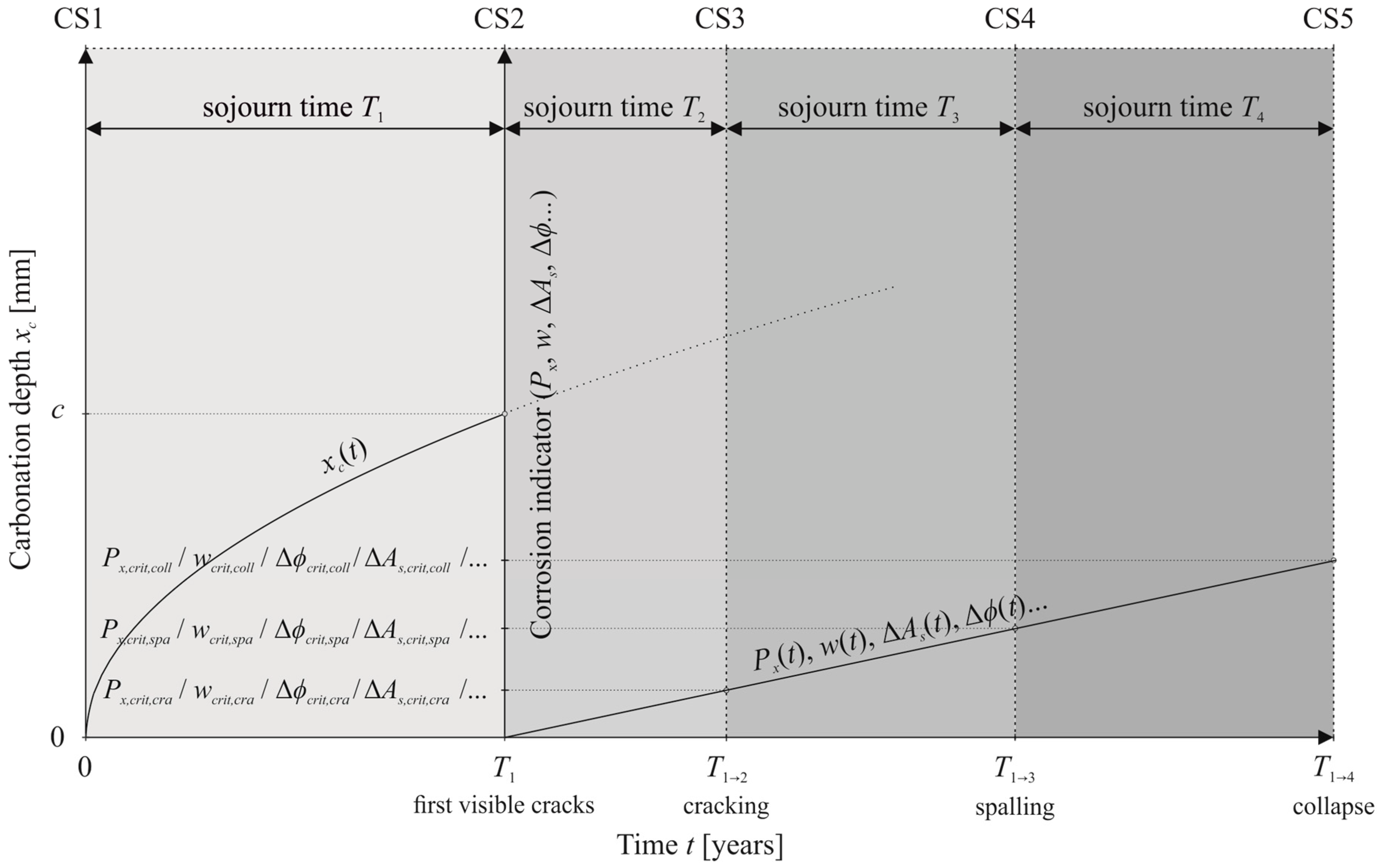
. The process of reinforcement corrosion can be roughly divided into two phases, which are called the initiation phase and the propagation phase [39]. Fib Bulletin 34 [7] defines the initiation as a phase that ends with the limit state of reinforcement depassivation being reached. The propagation phase is divided into limit states of crack formation, spalling of concrete cover, and collapse through bond failure or reduction of cross-section. In the following sections, analytical models describing these limit states are included.

3.1. Initiation Phase

The initiation phase of the process of carbonation-induced corrosion is marked by carbonation penetration, and it finishes roughly with the depassivation of reinforcement. Comprehensive descriptions of numerous analytical models of concrete carbonation and their development can be found in [40]. The analytical model that defines the limit state of carbonation-induced depassivation presented and applied in this article is supported by the fib [7,8,9]. The model was initially developed in the research projects DuraCrete [41] and DARTS [42]. In later development of the model, von Greve-Dierfeld and Gehlen [43] excluded the inverse carbonation resistance parameter R_NAC⁻¹ and introduced an additional parameter—carbonation rate k_NAC. The limit state equation of carbonation-induced depassivation, where the carbonation depth is compared with concrete cover, is given by Equation (11):

$$g\left(t\right)=c-x_c\left(t\right),$$

(11)

where:

• c is the concrete cover (mm), and
• x_c(t) is the carbonation depth at time t (mm).

Furthermore, carbonation depth can be expressed as:

$$x_c\left(t\right)=k_{NAC}·\sqrt{k_e·k_c·k_a}·\sqrt{t}·W\left(t\right),$$

(12)

where:

• k_NAC is the carbonation rate for standard test conditions (mm/years^0.5),
• k_e is the function describing the environmental effect of relative humidity,
• k_c is the function describing the effect of curing/execution,
• k_a is the function describing the effect of CO₂ concentration in the ambient air,
• t is time (year), i.e., the age of structure, and
• W(t) is the function describing the effect of wetting events.

The carbonation rate k_NAC in Equation (12) represents the resistance of the concrete mixture to carbonation, where the rate of the particular mixture is derived under constant (standard) test conditions. Tested values of carbonation rates of different concrete mixtures under standard test conditions can be found in [43,44,45]. The mean values of such tested carbonation rates are expressed as dependent on cement types, as shown in

Table 2. Mean values m of carbonation rate k_NAC (mm/years^0.5) for different combination of cement types and w/c ratios [46].

Cement Type	w/c Ratio
	0.40	0.45	0.50	0.55	0.60	0.65	0.70	0.75	0.80
CEM I	1	2	3	4	5	6	7	8	9
CEM II/A	1	2	3	4	5	6	7	8	9
CEM II/B	2	3	4	5	6	7	8	9	10
CEM III/A	2	3	4	5	6	7	8	9	10
CEM III/B	3	4	5	6	7	8	9	10	11

.

The shaded elements in Table 2 were obtained through linear extrapolation of measured values. Furthermore, von Greve-Dierfeld and Gehlen [43,44,45] consider that carbonation rate is normally distributed with the unique standard deviation s, which is unrelated to concrete mixture and is equal to 1.1 mm/years^0.5.

The environmental coefficient k_e introduces the effect of relative humidity on carbonation, and is described as:

$$k_e={\left(\frac{1-{\left(\frac{R{H}_a}{100}\right)}^{f_e}}{1-{\left(\frac{R{H}_l}{100}\right)}^{f_e}}\right)}^{g_e},$$

(13)

where:

• RH_a is the relative humidity of ambient air (%),
• RH_l is the reference (laboratory) humidity (%),
• f_e is the exponent (-), and
• g_e is the exponent (-).

As an input for the relative humidity RH_a, data from the nearest weather station may be used. Since relative humidity varies in a range from 0 to 100%, restricted distributions with an upper limit may be used to describe RH_a, such as beta or Weibull (max) distribution. The reference humidity RH_l has to be chosen in accordance with the test conditions to determine the carbonation resistance of the concrete. Since the carbonation rates presented in Table 2 were tested under standard test conditions, which imply relative humidity of 65 ± 5%, the reference humidity RH_l should be chosen within the range 60–70%. The parameters g_e and f_e have to be determined by means of a curve-fitting procedure with the actual test data. According to project DARTS [42], the best results are gained with f_e being equal to 5 and g_e being equal to 2.5.

Curing of newly built structures is performed to prevent the drying of fresh concrete, and as such, it affects the hydration, and subsequently the carbonation, of the concrete. This has a prevailing effect on carbonation, and it can be taken into account through the curing/execution coefficient k_c, expressed in Equation (14):

$$k_c={\left(\frac{t_c}{7}\right)}^{b_c},$$

(14)

where:

• t_c is the curing time (days), and
• b_c is the exponent (-).

The curing time t_c is considered a constant, the value of which should be derived from execution documents or valid standards at the time of construction. The value of the variable b_c was quantified in DARTS [42] as being normally distributed with a mean value m = −0.567 and standard deviation s = 0.024.

Coefficient k_a, shown in Equation (15), describes the relation of the ambient air CO₂ content C_a and the laboratory content C_l used for standard test purposes:

$$k_a=\frac{c_a}{c_l},$$

(15)

where:

• C_a is the CO₂ concentration of ambient air (kg/m³) or (vol. %), and
• C_l is the CO₂ concentration during concrete testing in laboratory (kg/m³) or (vol. %).

The ambient air CO₂ concentration depends on parameters such as traffic volume, CO₂ emission of local industry, atmospheric stability, wind speed, etc. [47]. Von Greve-Dierfeld and Gehlen [44] included assumed maximum and minimum CO₂ concentrations obtained from literature review, and divided these values between rural and urban locations, as shown in

Table 3. Assumed maximum and minimum CO₂ concentrations based on a literature review [44].

Exposure Class	Distribution	Location	Mean Value	Standard Deviation
XC1/XC2	Normal	indoor/e.g., foundation	0.036 ≤ µ ≤ 0.043	0.0010 ≤ σ ≤ 0.0080
XC3/XC4	Normal	rural	0.036 ≤ µ ≤ 0.042	0010 ≤ σ ≤ 0.0055
		urban	0.038 ≤ µ ≤ 0.043	0.0015 ≤ σ ≤ 0.0080

.

In wetting periods, concrete surface absorbs water and thus inhibits carbonation. To take into account the meso-climatic conditions due to wetting events, the time-dependent function was introduced [42], called the environmental or wetting function W(t):

$$W\left(t\right)={\left(\frac{t_0}{t}\right)}^{\frac{{\left(p_{dr}·ToW\right)}^{b_w}}{2}},$$

(16)

where:

• t₀ is the reference time (year),
• p_dr is the probability of driving rain (-),
• ToW is the time of wetness (-), i.e., days with daily rainfall ≥ 2.5 mm, and
• b_w is the regression exponent (-).

Parameters ToW and p_dr are introduced in order to take into account the wetness of concrete surfaces that are not horizontal. Time of wetness ToW represents a percentage of rainy days per year, where a rainy day is considered to be a day with a minimum amount of precipitation water of 2.5 mm. Probability of driving rain p_dr represents an average distribution of the wind direction during rain events, and it depends on the strength and direction of wind, the orientation of the structural element, etc. In addition, the weather function contains two model parameters, b_w and t₀, which were quantified in [42] based on the analysis of the performed tests. The regression exponent b_w is considered normally distributed with a mean value m = 0.446 and a standard deviation s = 0.163. The reference time, t₀, at which the analysis was performed is equal to 28 days, or can be expressed in years as 0.0767 years.

To use the model of carbonation-induced depassivation for determining sojourn times of the semi-Markov process, the model has to express the duration in which the element remains un-depassivated (i.e., the initiation duration t_ini). By converting Equation (12), the time of initiation can be expressed as shown in Equation (17):

$$t_{ini}={\left(\frac{k_{NAC}^2·k_e·k_c·k_a}{c^2}·t_0^w\right)}^{\frac{1}{\mathrm{w}-1}},$$

(17)

where:

$$w={\left(p_{dr}·ToW\right)}^{b_w}.$$

(18)

3.2. Propagation Phase

During the propagation phase, the process of reinforcement corrosion takes place, the rate of which is governed by the availability of water and oxygen on the steel surface [40]. The consequences of reinforcement corrosion are the cracking of the cover, loss of steel concrete bond, decrease of steel cross-section, and loss of steel ductility [48]. In fib Bulletin 34 [7], these consequences are contained in the limit states of crack formation, spalling of the concrete cover, and collapse. These limit states are divided into serviceability limit states (SLS), which include the events of crack formation and spalling, and the ultimate limit state (ULS), which includes the event of collapse in different modes. To differentiate among collapse modes, different robustness classes (ROC) are described in [7]. These classes are given in connection with a rough estimate on the percentage of cross-section loss ΔA_s that causes particular collapse modes, as presented in

Table 4. Robustness classes (ROC) in relation to cross-section loss [7].

Robustness Class (ROC)	Characteristics	Loss of Cross-Section ΔAs (%)
ROC 3	bending reinforcement outside of anchorage and laps	25
ROC 2	shear reinforcement, anchorage zones with confinement	15
ROC 1	anchorage zones without confinement	5

. In other words, sufficient reliability regarding the ULS could be achieved by adding the needed extra reinforcement (sacrificial cross-section) in the amount presented in Table 4. However, it should be noted that these values are a rough estimate and need to be confirmed by further research.

Propagation of corrosion can be observed through several performance indicators, including the corrosion depth P_x, rate of corrosion v_corr, loss of cross-section area ΔA_s, loss of bar diameter Δφ, concrete crack width w, and so on. The simplified model for determining the corrosion depth P_x(t) can be expressed as in Equation (19):

$$P_x\left(t\right)=t·v_{corr},$$

(19)

where:

• t is the time of propagation (year), and
• v_corr is the corrosion rate (mm/year).

The value of bar diameter φ(t) as function of time and corrosion depth can be calculated according to Equation (20):

$$\varphi \left(t\right)={\varphi }_0-\alpha ·P_x\left(t\right),$$

(20)

where:

• φ₀ is the initial bar diameter (mm), and
• α is the factor accounting the type of corrosion (pitting or homogeneous) (-).

Corrosion types can be divided into homogeneous (uniform) corrosion and pitting (localized) corrosion, which result from carbonation-induced depassivation and chloride-induced depassivation, respectively. For homogeneous corrosion, it is assumed that the factor accounting for the type of corrosion α ranges between 0 and 2. On the contrary, for chloride-induced corrosion, it can be as high as 10 [49]. Furthermore, the loss of bar diameter expressed in percentages Δφ(t) is given by Equation (21):

$$\mathsf{\Delta }\varphi \left(t\right)=100·\frac{{\varphi }_0-\varphi \left(t\right)}{{\varphi }_0}.$$

(21)

According to [41], the concrete crack width w(t) can be expressed in connection to corrosion depth P_x(t), as shown in Equation (22):

$$w\left(t\right)=w_0+\beta ·\left(P_x\left(t\right)·P_0\right),$$

(22)

where:

• w₀ is the crack width when it is visible (≈0.05) (mm),
• β is the parameter that controls the propagation (-), and
• P₀ is the loss of reinforcement bar diameter when crack width is visible (mm).

It should be noted that the correlation between concrete quality, corrosion rates and microenvironment has not yet been quantified in detail. This implies that reliable findings are lacking, which would connect critical values of performance indicators (P_x(t), w(t), ΔA_s(t), Δφ(t),…) at which the states of cracking, spalling and collapse are triggered. Hence, it is hard to accurately express the duration of different propagation periods. To overcome this problem, a questionnaire was organized by fib’s Task Group 5.6, in which experts all over the world gave their opinion on expected penetration depths and propagation periods in carbonation environment. The estimations were given within the exposure class XC4, for a reference temperature of T_ref = 293 K, assuming that depassivation had already occurred. Collected data were statistically elaborated and presented in [7], where the propagation periods were described by lognormal distribution, as shown in

Table 5. Duration of propagation periods t_prop linked to the events of cracking and spalling according to data presented in [7].

Event	Duration of Propagation Periods	Mean Value m	Standard Deviation s	Location Parameter µ	Scale Parameter σ
cracking	tprop,cra [year]	4.5	1.5	1.45	0.32
spalling	tprop,spa [year]	9.0	2.5	2.16	0.27

.

In cases where the average yearly temperature T_real of the object being investigated differs from 293 K, the values in Table 5 need to be adapted using the formula for the temperature dependence of reaction rates (Arrhenius equation) [50], as presented in Equation (23):

$$t_{prop}(T_{real})=\frac{t_{prop}(T_{ref})}{e^{b·(\frac{1}{T_{ref}}-\frac{1}{T_{real}})}},$$

(23)

where:

• t_prop(T_real) is the duration of propagation period based on real temperature T_real (year),
• t_prop(T_ref) is the duration of propagation period based on reference temperature T_ref (year),
• b is the regression parameter (b = 4900 K),
• T_ref is the reference temperature (T_ref = 293 K), and
• T_real is the average yearly ambient temperature of the object considered (K).

Furthermore, in addition to the duration of propagation periods, critical corrosion depths P_crit causing the events of cracking and spalling can also be extracted from [7], as presended in

Table 6. Critical corrosion depths P_crit linked to the events of cracking and spalling, according to data presented in [7].

Critical Corrosion Depth Pcrit	Mean m	Standard Deviation s	Location Parameter µ	Scale Parameter σ
Pcrit,cra [µm]	171.0	57.00	5.09	0.32
Pcrit,spa [µm]	342.0	95.00	5.80	0.27

.

4. Relationship between the Semi-Markov Process and the Carbonation-Induced Corrosion

To date, several researchers have discussed the possibility of enhancing statistical models based on condition ratings by using analytical deterioration models describing different phenomena. These enhancements were based on establishing a relationship between condition states (CS) and the performance indicators expressed by analytical models. Although condition states are usually assigned to different scales by different organizations, it can be noted that for the corrosion process, the condition scale with condition states from CS1 to CS5 is mostly used. CS1 denotes the first condition state, where the structure is considered to be without any damage, and CS5 denotes the worst condition, i.e., a structure with high chances of collapse. In the following text, examples of the relationship between statistical and analytical models are presented, accompanied by a description of the relationship proposed in the article.

Roelfstra [51] and Roelfstra et al. [52] performed simulations for different values of model parameters for the process of chloride-induced corrosion. The results were connected with condition states (CSs) defined in the Swiss bridge management system “KUBA-MS”, and the transition matrices in the Markov chain model were calibrated to fit simulation results. They connected the condition states with the chloride concentration C(c,t), bar diameter loss Δφ(t), and percentage of cross-section loss ΔA_s(t), as presented in

Table 7. Relationship between condition states and performance indicators of carbonation induced corrosion given in literature.

	According to Roelfstra et al. [52]	According to Lethanh et al. [55]
CS1	C(c,t) < 0.2 wt.%/c	C(c,t) < 0.24 wt.%/c
CS2	C(c,t) > 0.2 wt.%/c; Δφ(t) < 50 µm	0.24 wt.%/c < C(c,t) < 0.48 wt.%/c
CS3	50 µm > Δφ(t); ΔAs(t) < 10%	C(c,t) > 0.48 wt.%/c; w(t) < 0.25 mm
CS4	10% < ΔAs(t) < 25%	0.25 mm < w(t) < 0.5 mm
CS5	ΔAs(t) > 25%	w(t) > 0.5 mm

. Furthermore, Hallberg and Racutanu [6] presented a service-life performance analysis model based on the Markov chain model and different concrete degradation models. Puz and Radic [53] presented a homogeneous Markov processes model based on the exponential distribution, utilizing chloride-induced corrosion models to determine sojourn times. They established the relationship between states of the exponential Markov process and chloride-induced corrosion by dividing deterioration into four stages (protected, vulnerable, attacked, and damaged). For these stages, sojourn times were determined depending on the chloride concentration C(c,t) and cross-section reduction ΔA_s(t). Mizutani et al. [54] and Lethanh et al. [55] proposed to estimate the transition probabilities in the Markov chain from a chloride-ingress model, which they refer to as the mechanistic-empirical model. In their work, they established the relationship by dividing the process of chloride ingress into two phases, depending on chloride content C(c,t), and the process of corrosion into three phases, depending on crack width w(t), as presented in Table 7.

In the framework presented in this article, the choice of which exact performance indicator of corrosion propagation (P_x(t), ΔA_s(t), Δφ(t), w(t)...) should be used to denote the beginning and the end of certain condition state is left open. In the article, only the simplest analytical models of corrosion propagation are presented, which do not account for more complicated processes, such as the influence of traffic load on corrosion acceleration. For example, in cases where infrastructure operators possess a great amount of data on traffic load and proper analytical models that would connect this data to corrosion acceleration, they can easily implement it within the framework presented in this article. Taking the stated into account, the relationship between the semi-Markov process and carbonation-induced corrosion can be established as presented in Figure 1.

In the upper part of Figure 1, condition states (CSs) obtained during visual inspections are assigned, thereby defining the limits of sojourn times T_i. Additionally, in the lower part of Figure 1, periods of carbonation-induced corrosion are depicted together with points in time that denote the sums of sojourn times T_1→k. As can be seen, depassivation of reinforcement defines the end of the first sojourn time T₁, and it is considered to be equivalent in time to the occurrence of first visible cracks (w₀ ≈ 0.05 mm). This is done since depassivation itself cannot be detected during a visual inspection, and the occurrence of the first visible cracks can be expected relatively shortly after depassivation. The second sojourn time T₂ is the time from the occurrence of the first visible cracks until the state of severe cracking, meaning that the sum of sojourn times T_1→2 = T₁ + T₂ denotes the whole time from construction until the state of cracking. The state of cracking has been defined as a point in time at which a chosen indicator of corrosion propagation (P_x(t), ΔA_s(t), Δφ(t), w(t)…) reaches its defined critical value (P_x,crit,cra, ΔA_s,crit,cra, Δφ_crit,cra, w_crit,cra…). Following the same analogy, the sum of sojourn times T_1→3 denotes the time until spalling, and T_1→4 denotes the time until collapse.

5. Case Study

5.1. Austrian Federal Railway (ÖBB)

As of January 2016, the Austrian Federal Railway (ÖBB) had an infrastructure network of 9,108 bridges in total. Bridge stock of the ÖBB in 2016 is presented in

Table 8. Bridge stock of the ÖBB in 2016, arranged according to their general function.

Bridge Type	Railway	Culvert	Road	Pedestrian	Other	Total
Bridge Number	5 406	2 781	643	68	210	9 108

, arranged according to general function.

Concrete and reinforced concrete bridges of the ÖBB network were erected in high frequency from 1945 onwards. As an outcome, today the ÖBB bridge stock is predominantly composed of reinforced concrete, as shown in

Table 9. Bridge distribution by material in the ÖBB bridge stock in 2016 [46].

Material	Reinforced concrete	Stone and brick	Steel
Percentage of Bridges	70%	17%	13%

.

Periodical visual inspection in ÖBB is carried out every two to three years, depending on the age of the structure. In the course of assessment, the inspector assesses the damage found and determines the measures to be implemented [56]. Moreover, a condition rating is assigned and documented in a report, based on a grading system with classes (states) 1 to 5, as presented in

Table 10. Condition rating system used by the ÖBB, with assigned condition, restriction, and action for each class [5].

Class	Condition State (CS)	Condition and Restrictions	Action
Class 1	CS1	Very good condition, no restrictions	No actions
Class 2	CS2	Good state of preservation, no restrictions	No actions
Class 3	CS3	Poor state of preservation, no restrictions	Subjected to repair
Class 4	CS4	Very poor state of preservation, no restrictions	Subjected to repair—sometimes also renewal
Class 5	CS5	Very poor state of preservation, immediate restrictions	Subjected to renewal

. Since it consists of five condition states, the condition state grading system coincides with the established relationship between the phases of the carbonation-induced corrosion and sojourn times of the semi-Markov process, as presented in Figure 1.

5.2. Weikendorf Bridge

The framework presented in the previous chapters is implemented in a case study of the Weikendorf railway bride, which belongs to the Austrian Federal Railway (ÖBB). The bridge is a single-span plate girder bridge made of reinforced concrete, and was built in 1967 on the route Gänserndorf–Marchegg in the state of Lower Austria. In 2014, the bridge was repaired, as can be seen in Figure 2.

From screening design documents, it can be seen that the bridge was erected using concrete classes B160, B225, and B400, according to the norm ÖNORM B 3302 [57]. The cross-section of the bridge is depicted in Figure 3, where a concrete class is associated with each element, as given in design documents.

In

Table 11. Prescribed w/c ratios in connection to concrete classes and cement strength classes [58].

Element	Label	Concrete Class ÖNORM B 3302 [57]	w/c Ratio Range [58]	Concrete Class ÖNORM B 4710-1 [59]
Wings	W	B160	0.74–1.03	C12/15
Abutments	A	B160	0.74–1.03	C12/15
Edge beams	EB	B225	0.61–0.88	C16/20
Girder	G	B400	0.32–0.64	C30/37

, for the concrete classes envisaged in the design documents, the prescribed w/c ranges are presented according to [58]. Additionally, currently used concrete classes are assigned according the standard ÖNORM B 4710-1 [59].

From the elements of the bridge presented in Table 11, only the wings are exposed to rain, and hence can be considered in the class XC4. Due to the fact that durations of propagation periods t_prop, presented in Table 5, were given only for exposure class XC4, only the wings of the bridge could be analyzed.

5.3. Visual Inspection

The condition states (ratings) introduced in Table 9 are assigned based on the results of visual inspections, which are commonly carried out by teams of trained technicians. During visual inspection, they try to detect defects and damage, and, depending on their extent, assign the aforementioned condition state. Furthermore, visual inspection comprises the use of only simple tools such as hammers to remove cracked parts of concrete, rebound hammers to detect areas with lower compressive strength, etc. During the inspections, the following is therefore recorded: (i) the identified defects and damages, such as cracks, concrete spalling, steel corrosion, etc., (ii) the required immediate intervention measures, (iii) the reparability of the observed defects and damage, and (iv) the comparison of the existing condition of the structure with the previously recorded one. Accordingly, in 2005, the Weikendorf Bridge was assigned the condition state CS3, due to several damage zones with spalled parts of concrete, primarily in the abutments and wings. The same condition state was assigned in subsequent inspections, until 2014, when the bridge was repaired. Before 2005, inspection records contained only a description of the condition, without a condition state being assigned. Following the inspection in 2013, it was decided that additional testing should be performed, such as determining compressive strength, measuring reinforcement properties, measuring carbonation depth, etc. From the performed tests, it was found that the abutments exhibited high levels of chloride and carbonation, and the wings exhibited high levels of carbonation.

Taking into account the condition state grading system of five states, the state of the process at time t = 38 years (in 2005) can be denoted by an n-dimensional vector p(38). Thus, Equation (1) takes the form:

$$p\left(38\right)=\left[p_1\left(38\right)p_2\left(38\right)p_3\left(38\right)p_4\left(38\right)p_5\left(38\right)\right].$$

(24)

Furthermore, if the fact that the structure is graded to be in CS3 at the age of 38 years is taken with certainty, the probability vector denoting the state of the process becomes:

$$p\left(38\right)=\left(0 0 1 0 0\right).$$

(25)

However, such representation implies that no uncertainty is connected with the result of visual inspection. This is presumed, since a condition rating is usually assigned as a deterministic value, making it hard to allocate a level of uncertainty to such a condition state. If, for example, an indication were to exist that the visual inspection was performed with ±15% of accuracy, the probability vector denoting the state in Equation (25) could be formed as p(38) = (0 0 0.15 0.70 0.15).

5.4. Carbonation Measurements

Carbonation depth was tested by applying the phenolphthalein indicator solution in the abutments, wings, edge beam and deck. The sketch of measuring the carbonation depth in the abutments and wings can be seen in Figure 4.

The results of the measurements are presented in

Table 12. Results of measuring carbonation depth x_c(46) in the Weikendorf bridge, for wings (W), abutments (A), edge beam (EB) and girder (G).

Point	Height (m)	Exposure Class	Measured Value (mm)
W1	1.50	XC4	15
W2	1.50	XC4	23
W3	1.50	XC4	16
W4	1.50	XC4	43
A1	0.20	XC3	38
A2	1.30	XC3	49
A3	2.35	XC3	52
A4	3.40	XC3	20
A5	3.40	XC3	18
A6	2.35	XC3	25
A7	1.30	XC3	46
A8	0.20	XC3	37
EB1	>4.00	XC4	1
G1	>4.00	XC3	1

. An associated exposure class was assigned to each measurement location.

In addition to measuring carbonation depth, properties of reinforcement (such as concrete cover, raster and diameter) were determined using a concrete scanner for non-destructive structural inspection. According to the performed tests and the design documents, the properties of reinforcement in the bridge wings can be obtained as given in

Table 13. Properties of reinforcement in bridge wings, grasped from design documents and performed tests.

Values	Horizontal Reinforcement	Vertical Reinforcement
concrete cover [mm]	circa 30	circa 40
raster [cm]	15	20
diameter [φ]	14	12

.

These properties are relevant in order to determine the duration of both the initiation and propagation phases. The representation of the measured carbonation depths, as well as the reinforcement properties, can be seen in Figure 5.

5.5. Carbonation Propagation

To determine the duration of the initiation phase t_ini, first the parameters in Equation (17) have to be determined. Some of these parameters are constants, and others can be obtained from design documents, performed inspections, meteorological data, literature survey, etc. Moreover, results of measured carbonation depth can serve for the crosschecking of such determined parameters. Alternatively, when substantial information related to the measured carbonation depth is known, a Bayesian updating procedure can be used to directly update the initially assumed carbonation depth.

Time of wetness ToW was determined based on historical measurements obtained from the weather stations in Gänserndorf, located 1.45 km from the bridge [59]. Precipitation data were available for each day from 1971 to 2014. From the data, the average number of rainy days for each year was calculated, and expressed as a percentage. Rainy days were divided into days with more than 2.5 mm of rainfall and those with more than 0 mm of rainfall, as presented in Figure 6.

Furthermore, the mean value of precipitation > 2.5 mm for all average yearly values in the period 1971–2014 was calculated and depicted. This value is equal to 0.145, and it was used as the ToW of the Weikendorf Bridge. On the other hand, relative humidity RH_a of the ambient air could not be determined as precisely as the time of wetness, since the closest weather station available is located 20 km from the bridge. For this reason, all available weather stations in the state of Lower Austria were analyzed based on the measurements of the Central Institute for Meteorology and Geodynamics [60], as depicted in Figure 7. Data were available in the form of average humidity for the whole period 1981–2010, measured at 7:00 a.m. and 2:00 p.m. When different stations are analyzed, considering an average value between 7:00 AM and 2:00 PM, the data exhibit a mean value of 72.37% and a standard deviation of 2.23%.

As stated in the previous chapters, the probability of driving rain p_dr represents an average distribution of the wind direction during rain events, and it depends on the strength and direction of the wind, the orientation of the structural element, etc. From the available meteorological data, it was not possible to compare exact precipitation and wind directions. However, being mostly sheltered by the embankment, the wings are considered to have a low probability of driving rain. Hence, a probability of driving rain of p_dr = 0.1 was used for the analysis.

No concrete cover c was found to be assigned in the design documents, while the tested concrete cover in the test report was only assigned approximately, as shown in Table 13. In fib Bulletin 34 [7], it is stated that that the observed standard deviations of concrete cover obtained from field measurements range from 2 mm ≤ s ≤ 15 mm. Moreover, deviation in concrete cover can be associated with level of quality control, e.g., the coefficient of variation can be assumed to be 15% in structures with high quality control, 20% in structures with medium, and 30% in those with low quality control. Since the wings of the Weikendorf bridge are considered to be constructed with medium quality control, the concrete cover was assumed to be normally distributed with the mean value of 30 mm, coefficient of variation of 20%, and standard deviation of 6 mm.

Carbonation rate k_NAC was determined based on Table 2, considering that according to the design documents, the concrete class B160 was used in the wings. A w/c ratio of 0.75 and the cement type CEM I were assumed, in the belief that this cement type was most common at the time of construction. Such presumed parameters resulted in normally distributed carbonation rate k_NAC with a mean value of 8.0 and a standard deviation of 1.1.

It is not known which exact cement strength class was used, nor what the ambient temperature was during construction. However, since the resistivity of the concrete was proven to be low by the performed test, a short curing time is assumed, i.e., t_c of 2 days.

The value of carbonation concentration of ambient air C_a was taken to be the maximum proposed for rural areas, thus being normally distributed with the mean value of 0.042% and a standard deviation of 0.005.

The overall parameters for the carbonation-induced depassivation model gathered for the wings of the Weikendorf Bridge are presented in

Table 14. Parameters of carbonation-induced depassivation for the wings of the Weikendorf Bridge.

Parameter		Unit	Distribution Type	Mean Value m	Standard Deviation s
Relative humidity—laboratory	RHl	%	Constant	65	-
Exponent	fe	-	Constant	5	-
Exponent	ge	-	Constant	2.5	-
Regression exponent	bw	-	Lognormal	0.446	0.163
Exponent	bc	-	Normal	−0.567	0.024
Reference time	t0	years	Constant	0.0767	-
CO2 concentration—laboratory	Cl	vol.%	Constant	0.04	-
Concrete cover	c	mm	Normal	30	6
Relative humidity of ambient air	RHa	%	Normal	72.4	2.2
Time of wetness	ToW	%	Constant	0.145	-
Probability of driving rain	pdr	%	Constant	0.10	-
Carbonation rate	kNAC	mm/years0.5	Normal	8	1.1
Curing time	tc	days	Constant	2	-
CO2 concentration of ambient air	Ca	vol.%	Normal	0.042	0.005

.

Carbonation depth at the age 46 years x_c(46) calculated using the parameters in Table 14 resulted in a mean value of 40.80 mm and a standard deviation of 13.87 mm. Such calculated results closely match the highest measured value of carbonation in point W4, as presented in Table 12. Moreover, from the parameters shown in Table 14, using Equation (17), it is possible to calculate the duration of time of initiation t_ini. For the probabilistic analysis of time of initiation t_ini, as well as for other probabilistic analysis in the article, the probabilistic engine FReET (Feasible Reliability Engineering Tool) was used [61]. The determined statistical parameters of the duration of time of initiation t_ini are presented in

Table 15. Duration of time of initiation t_ini of the process of carbonation-induced corrosion for the wings of the Weikendorf Bridge.

Phase (state)	Mean m	Standard Deviation s	Location Parameter µ	Scale Parameter σ
tini [year]	11.08	9.84	2.11	0.76

as lognormally distributed. As shown in Figure 1, the time of initiation t_ini represents the sojourn time of condition state one T₁ of the semi-Markov process.

5.6. Corrosion Propagation

Historical measurements of temperature from the Central Institute for Meteorology and Geodynamics in Austria served for determining the ambient temperature of the Weikendorf Bridge [60]. The data consisted of the mean temperature of the period 1961–1990 for weather stations in Lower Austria. Available data were analyzed, where data from the Gänsendorf weather station in the near vicinity of the bridge also exist. Hence, for the parameter T_real in Equation (23), the mean value of 282.4 K for the Gänsendorf station was taken into account, with the standard deviation obtained by analysis of different stations. When different stations were analyzed, as presented in Figure 8, a standard deviation of 1.2 K was obtained.

Using Equation (23), the duration until events of cracking and spalling t_prop for the Weikendorf Bridge can be recalculated. The results of the recalculation are presented in

Table 16. Values of duration of propagation t_prop until the occurrence of events of cracking and spalling for the wings of the Weikendorf Bridge.

Event	tprop	Mean Value m	Standard Deviation s	Location Parameter µ	Scale Parameter σ
cracking	tprop,cra	8.46	2.89	2.08	0.33
spalling	tprop,spa	16.91	4.87	2.79	0.28

as lognormally distributed.

Taking into account the values presented in Table 6 and Table 16, and using Equation (19), it is possible to determine the approximate corrosion rate v_corr in the wings as an average between corrosion rates causing cracking and spalling. The mean value of approximate corrosion rate v_corr in wings was determined to be equal to 22.2 µm/year, with a standard deviation of 10.0 µm/year.

Since the wings are elements that exhibit lower consequences once the failure has occurred, the robustness class ROC 3 (presented in Table 4) was chosen to represent the appropriate failure mode for the wings. This means that the loss of cross-section ΔA_s of 25% is deemed to cause collapse. Due to the fact that horizontal reinforcement has a smaller concrete cover c (i.e., approximately 30 cm), it is expected that it will be the first to be affected by corrosion. The diameter of the horizontal reinforcement is 14 mm. P_crit,coll was obtained assuming homogeneous corrosion with α = 2 and employing Equation (20), as shown in

Table 17. Critical corrosion depth P_crit,coll for ROC3, derived for bridge wings.

Robustness Class (ROC)	Loss of Cross-Section ΔAs (%)	Critical Corrosion Depth	Value (µm)
ROC 3	25	Pcrit,coll	937.82

.

Taking into account critical corrosion depth P_crit,coll and corrosion rate v_corr, the duration of propagation until the event of collapse t_prop,coll can be calculated. To do so, Equation (19) and the reinforcement properties given in Table 13 need to be used. The calculated values for duration until the event of collapse are shown in

Table 18. Duration of propagation until the event of collapse t_prop,coll.

Robustness Class (ROC)	Phase	Mean Value m	Standard Deviation s	Location Parameter µ	Scale Parameter σ
ROC 3	tprop,coll	50.82	22.89	3.84	0.43

.

5.7. Condition Prediction

Once the input parameters are determined, it is possible to perform the analysis using the semi-Markov process model. To do so, the sums of the sojourn times $T_{1\to i}$. have to be numerically determined. These sums for the wings of the Weikendorf Bridge are presented in

Table 19. Sums of sojourn times $T_{1\to i}$. of the process of carbonation-induced corrosion in the wings of the Weikendorf Bridge.

${\mathit{T}}_{1\to \mathit{i}}$	Σ t	Mean Value m	Stdard Deviation s	Location Parameter µ	Scale Parameter σ
$T_{1\to 2}$	tini + tprop,cra	19.54	125	2.85	0.49
$T_{1\to 3}$	tini + tprop,spa	27.99	197	3.26	0.38
$T_{1\to 4}$	tini + tprop,coll	61.90	24.91	4.05	0.39

.

The PDFs and SFs (in Equations (7)–(11)) of the sojourn time sums $T_{1\to i}$ were used to calculate single-time step transition probabilities p_ij^t,t+1. For instance, the probability of transition from the state 3 to 4 in the period between the 38th and 39th year is given in Equation (26):

$$p_{3,4}^{38,39}=\frac{f_{1\to 3}\left(38\right)}{S_{1\to 3}\left(38\right)-S_{1\to 2}\left(38\right)}=0.1470.$$

(26)

Once all the single-time step probabilities are known, it is possible to populate the transition matrices P^t,t+1, as shown for the probability matrix P^38,39 in Equation (27):

$$P^{38,39}=\left[\begin{array}{ccccc}{p}_{1,1}^{38,39}& p_{1,2}^{38,39}& 0& 0& 0\\ 0& p_{2,2}^{38,39}& p_{2,3}^{38,39}& 0& 0\\ 0& 0& p_{3,3}^{38,39}& p_{3,4}^{38,39}& 0\\ 0& 0& 0& p_{4,4}^{38,39}& p_{4,5}^{38,39}\\ 0& 0& 0& 0& 1\end{array}\right]=\left[\begin{array}{ccccc}0.918& 0.081& 0& 0& 0\\ 0& 0.674& 0.326& 0& 0\\ 0& 0& 0.853& 0.147& 0\\ 0& 0& 0& 0.981& 0.019\\ 0& 0& 0& 0& 1\end{array}\right].$$

(27)

The probability that the process will assume one of the states i in the subsequent time period k can be calculated using Equation (3). For instance, when predicting the condition of the wings at the age t = 38 years for the subsequent period k of 20 years, the n-dimensional vector expressed in Equation (3) takes the form:

$$p\left(58\right)=p\left(38\right)·P^{38,39}·P^{39,40}\dots P^{57,58}=\left[0 0 0.034 0.626 0.340\right].$$

(28)

The obtained values in Equation (28) show that the probabilities that the wings will be in each one of five possible condition states in the year 2025 are equal to p₁(58) = p₂(58) = 0%, p₃(58) = 3.4%, p₄(58) = 62.6%, and p₅(58) = 34.0%.

After all the transition matrices P^t,t+1 are known, it is possible to analyze the condition of the wings for all subsequent periods k, as depicted in Figure 9a.

The shaded part of Figure 9a presents the elapsed time, i.e., the time before the inspection in 2005 when the CS3 was first assigned. If the same structure is regarded as newly built, then the state condition vector takes the form p(0) = (1 0 0 0 0). Applying such a state condition vector, the conditions for the subsequent periods k were obtained, as depicted in Figure 9b. One can easily notice that if the structure is observed as new, the most probable condition state at the time t = 38 years is CS4, in contrast to CS3, which was assigned based on visual inspection at the age of 38 years.

6. Discussion of Results

Several assumptions were made in the process of implementing the framework in the Weikendorf Bridge. Along with a discussion of the obtained results, this chapter provides clarification for some of these assumptions, as well as a study of their effect on the obtained results. One of the stated assumptions is that the highest measured carbonation depth should trigger corrosion first, which does not have to be the case. Due to this assumption, the parameters in Table 14 were chosen so that they match the highest measured value in point W4, thus influencing the subsequently determined t_ini. However, when the mean of the measured values presented in Table 12 is observed, the duration of the initiation phase t_ini becomes significantly longer than the one obtained in Table 15. Hence, in order to understand the influence of duration of initiation phase, the range of mean values of t_ini = 20, 30...100 years, with the coefficient of variation c_v = 0.5, was analyzed. Figure 10 depicts the probabilities that the process will assume one of the condition states i for the subsequent period k = 50 years, taking into account the condition state CS1 at the age of 0 years.

Other important implications assumed in the article are the corrosion rate v_corr and duration of propagation periods being based on recommendations given in [7]. These recommendations lead to the mean value of corrosion rate v_corr = 22 µm/year being used in the analysis. However, according to [62], corrosion rates higher than 1 μA/cm² (≈ 16 µm/year) are seldom measured, while values between 0.1–1.0 μA/cm² (≈ 1.6–16.0 µm/year) are the most frequent. Therefore, the mean corrosion rate was altered in the range v_corr = 4, 8,...16 µm/year, with coefficient of variation c_v = 0.5, in order to understand the behavior of the process for lower corrosion rates. For such ranges of corrosion rates, the probabilities that the process will assume one of the condition states i for the subsequent period k = 50 years, taking into account the condition state CS1 at an age of 0 years, are depicted in Figure 11. As can be seen in Figure 11, the probabilities of collapse for the corrosion rate v_corr < 4 µm/year are almost equal to zero for the first 50 years.

The analysis of the duration of the collapse period was performed for the robustness class ROC3, which assumes a 25% cross-section loss, as presented in Table 17 and Table 18. However, it should be noted that different collapse modes are possible in other bridge elements.

It is important to mention that due to lack of data before 2005, it was assumed that the bridge entered in CS3 in 2005 and stayed in the same state until the last inspection in 2013, before it was repaired. Nonetheless, it is possible that the bridge was already in the state CS3 prior to inspection in 2005. For this reason, to account for the recorded (past and present) duration of the bridge being in a certain state, sojourn times of these states have to be adjusted according to records.

When analyzing the obtained results presented in Figure 9, one has to bear in mind that these results show the condition forecast only for the case of carbonation-induced corrosion. However, the Weikendorf Bridge was affected with other deterioration processes, as well, such as chloride ingress. In fact, very often a structure is affected by multiple deterioration processes at once. Unfortunately, the combined effects of various deterioration processes have not yet been studied in detail. Hence, at the moment, to account for multiple deterioration processes, only possible solution is to summon the probabilities of reaching the same condition state caused by different processes.

7. Summary and Conclusions

The article presented a framework for condition prediction of existing concrete bridges, using a combination of the semi-Markov process as a statistical model and carbonation-induced corrosion as an analytical model. As such, the framework should assist engineers and operators in condition assessment of large number of bridges in infrastructural networks, as well as in optimizing the scheduling of interventions. In the framework, the condition is forecasted in the form of the probability that the bridge (process) will assume one of condition states i in a given subsequent period, by using the sojourn times derived from analytical deterioration models.

The distinctiveness of the presented framework and its contribution to the state-of-the-art in bridge management and condition prediction are that:

• the framework takes into account the probabilistic nature of the deterioration process, as well as the historic deterioration path, through PDFs and SFs of the sum of sojourn times presented in Equation (6). In this way, the framework does not just consider the present condition, but rather the sequence of events that preceded it. In other words, the semi-Markov process does not exhibit the ‘memoryless’ assumption, which is an important property of the Markov chain model;
• by estimating the transition probabilities in the transition matrix P^t,t+1 based on analytical models of deterioration, the framework is suitable for bridge inventory where reliable data on condition states are lacking, which is very often the case for condition data related to advanced deterioration [63];
• the framework overcomes other shortcomings of the homogeneous Markov chain, such as discrete transition time intervals, constant bridge population, and stationary transition probabilities;
• it is a holistic framework in the sense that it utilizes all the available data, such as environmental loading, material properties, structural parameters, etc., and not just condition ratings from visual inspections. This data can be acquired from literature survey, standards valid at the time of design and construction, design documents, inspection documents, test and monitoring reports, empirical knowledge of experts, and so on;
• although the article concentrates on concrete bridges and the process of carbonation-induced corrosion, it is flexible to implementation on any structural or material type, as well as any deterioration process for which an adequate deterioration model exists;
• by considering both deterioration path and bridge properties, the framework can highlight groups of structures with similar properties, and in this way differentiate those with a high rate of deterioration from those deteriorating at a slower pace.

Altogether, it can be concluded that the enclosed framework presents a suitable alternative to presently implemented frameworks for condition prediction used in Bridge Management Systems.

References

1. Mirzaei, Z.; Adey, B.T. Investigation of the use of three existing methodologies to determine optimal life-cycle activity profiles for bridges. Struct. Infrastruct. Eng. 2015, 11, 1484–1509. [Google Scholar] [CrossRef]
2. Bortot, F.; Zonta, D.; Zandonini, R. A bridge management strategy based on future reliability and semi-Markov deterioration models. In Proceedings of the 3rd International ASRANet Colloquium, Glasgow, UK, 10–12 July 2006; ASRANet Ltd.: Glasgow, UK, 2006. [Google Scholar]
3. Pnevmatikos, N.G.; Hatzigeorgiou, G.D. Damage detection of frame structures subjected to earthquake excitation using discrete walvet analysis. Bull. Earthq. Eng. 2016, 15, 227–248. [Google Scholar] [CrossRef]
4. Pnevmatikos, N.G.; Blachowski, B.; Hatzigeorgiou, G.D.; Swiercz, A. Wavelet analysis based damage localization in steel frames with bolted connections. Smart Struct. Syst. 2016, 18, 1189–1202. [Google Scholar] [CrossRef]
5. Zambon, I.; Vidovic, A.; Strauss, A.; Matos, J.; Friedl, N. Prediction of the remaining service life of existing concrete bridges in infrastructural networks based on carbonation and chloride ingress. Smart Struct. Syst. 2018, 21, 305–320. [Google Scholar] [CrossRef]
6. Hallberg, D.; Racutanu, G. Development of the Swedish bridge management system by introducing a LMS concept. Mater. Struct. 2007, 627–639. [Google Scholar] [CrossRef]
7. fib Bulletin 34. Model Code for Service Life Design of Concrete Structure; Model code prepared by Task Group 5.6; International Federation for Structural Concrete (fib): Lausanne, France, 2006. [Google Scholar]
8. fib Model Code for Concrete Structures; International Federation for Structural Concrete; Wilhelm Ernst & Sohn: Berlin, Germany, 2010.
9. fib Bulletin 59. Condition Control and Assessment of Reinforced Concrete Structures Exposed to Corrosive Environment (Carbonation/Chlorides); International Federation for Structural Concrete: Lausanne, France, 2011. [Google Scholar]
10. fib Bulletin 76. Benchmarking of Deemed-to-Satisfy Provisions in Standards: Durability of Reinforced Concrete Structures Exposed to Chlorides; Document Competence Center Siegmar Kästl e.K: Ostfildern, Germany, 2015. [Google Scholar]
11. Agrawal, A.K.; Kawaguchi, A.; Chen, Z. Deterioration Rates of Typical Bridge Elements in New York. J. Bridge Eng. 2010, 15, 419–429. [Google Scholar] [CrossRef]
12. Zambon, I.; Vidovic, A.; Strauss, A.; Matos, J.; Amado, J. Comparison of Stochastic Prediction Models Based on Visual Inspections of Bridge Decks. J. Civ. Eng. Manag. 2017, 23, 553–561. [Google Scholar] [CrossRef]
13. Ang, A.H.S.; Tang, W.H. Probability Concepts in Engineering Planning and Design, Basic Principles, 2nd ed.; Wiley: Hoboken, NY, USA, 2007. [Google Scholar]
14. Wang, J.; Liu, X. Evaluation and Bayesian dynamic prediction of deterioration of structural performance. Struct. Infrastruct. Eng. 2010, 6, 663–674. [Google Scholar] [CrossRef]
15. Jacinto, L.; Neves, L.C.; Oliveir, L. Bayesian assessment of an existing bridge: A case study. Struct. Infrastruct. Eng. 2015, 12, 61–77. [Google Scholar] [CrossRef]
16. Zanini, M.A.; Faleschini, F.; Pellegrino, C. Bridge residual service-life prediction through Bayesian visual inspection and data updating. Struct. Infrastruct. Eng. 2017, 13, 906–917. [Google Scholar] [CrossRef]
17. Sobanjo, J.O. A neural network approach to modeling bridge deterioration. In Proceedings of the 4th Congress of Computing in Civil Engineering, Philadelphia, PA, USA, 16–18 June 1997; ASCE: Philadelphia, PA, USA, 1997; pp. 623–626. [Google Scholar]
18. Arima, H.; Tanaka, S.; Matsui, S. Maintenance system of paint on steel bridges. Technol. Rep. Osaka Univ. 1999, 49, 171–178. [Google Scholar]
19. Huang, Y.H. Artificial Neural Network Model of Bridge Deterioration. J. Perform. Constr. Facil. 2010, 24, 597–602. [Google Scholar] [CrossRef]
20. Sasmal, S.; Ramanjaneyulu, K.; Gopalakrishnan, S.; Lakshmanan, N. Fuzzy Logic Based Condition Rating of Existing Reinforced Concrete Bridges. J. Perform. Constr. Facil. 2006, 20, 261–273. [Google Scholar] [CrossRef]
21. Mitra, G.; Jain, K.K.; Bhattacharjee, B. Condition Assessment of Corrosion-Distressed Reinforced Concrete Buildings Using Fuzzy Logic. J. Perform. Constr. Facil. 2010, 24, 562–570. [Google Scholar] [CrossRef]
22. Furuta, H.; Kameda, T.; Nakaha, K.; Takahashi, Y.; Frangopol, D.M. Optimal bridge maintenance planning using improved multi-objective genetic algorithm. Struct. Infrastruct. Eng. 2006, 2, 33–41. [Google Scholar] [CrossRef]
23. Rashedi, R.; Hegazy, T. Capital renewal optimization for large-scale infrastructure networks: Genetic algorithms versus advanced mathematical tools. Struct. Infrastruct. Eng. 2015, 11, 253–262. [Google Scholar] [CrossRef]
24. Ghodoosi, F.; Abu-Samra, S.; Zeynalian, M.; Zayed, T. Maintenance Cost Optimization for Bridge Structures Using System Reliability Analysis and Genetic Algorithms. J. Constr. Eng. Manag. 2018, 144. [Google Scholar] [CrossRef]
25. Kobayashi, K.; Kaito, K.; Lethanh, N. A statistical deterioration forecasting method using hidden Markov model for infrastructure management. Transp. Res. Pt. B Methodol. 2012, 46, 544–561. [Google Scholar] [CrossRef] [Green Version]
26. Lethanh, N.; Kaito, K.; Kobayashi, K. Infrastructure Deterioration Prediction with a Poisson Hidden Markov Model on Time Series Data. J. Infrastruct. Syst. 2015, 21. [Google Scholar] [CrossRef]
27. Corotis, R.B.; Ellis, J.H.; Jiang, M. Modeling of risk-based inspection, maintenance and life-cycle cost with partially observable Markov decision processes. Struct. Infrastruct. Eng. 2005, 1, 75–84. [Google Scholar] [CrossRef]
28. Faddoul, R.; Raphael, W.; Chateauneuf, A. A generalised partially observable Markov decision process updated by decision trees for maintenance optimisation. Struct. Infrastruct. Eng. 2011, 7, 783–796. [Google Scholar] [CrossRef]
29. Schöbi, R.; Chatzi, E.N. Maintenance planning using continuous-state partially observable Markov decision processes and non-linear action models. Struct. Infrastruct. Eng. 2016, 12, 977–994. [Google Scholar] [CrossRef]
30. Puz, G.; Radic, J.; Stipanovic-Oslakovic, I. A New Model for Stochastic Analysis of Bridge Durability. J. Croat. Assoc. Civ. Eng. 2010, 62, 287–297. [Google Scholar]
31. Wallbank, E.J. The Performance of Concrete in Bridges a Survey of 200 Highway Bridges; HMSO: London, UK, 1989. [Google Scholar]
32. Henriksen, C.F.; Stoltzner, E. Chloride Corrosion in Danish Road-Bridge Columns. Concr. Int. 1993, 55–60. [Google Scholar]
33. Schießl, P.; Mayer, T.F. Schlussberichte zur ersten Phase des DAfStb/BMBF-Verbundforschungsvorhabens, Nachhaltig Bauen mit Beton; Schriftenreihe des Deutschen Ausschusses für Stahlbeton: Berlin, Germany, 2007; Nr. 572. (In German) [Google Scholar]
34. Ng, S.K.; Moses, F. Bridge deterioration modelling using semi-Markov theory. In Proceedings of the Structural Safety and Reliability, Shiraishi, Shinozuka & Wen, Rotterdam, The Netherlands, 1 January 1998; Balkema: Rotterdam, The Netherlands, 1998; pp. 114–120. [Google Scholar]
35. Kleiner, Y. Scheduling inspection and renewal of large infrastructure assets. J. Infrastruct. Syst. 2001, 7, 136–143. [Google Scholar] [CrossRef]
36. Mašović, S.; Stošić, S.; Hajdin, R. Application of Semi-Markov Decision Process in Bridge Management. In Proceedings of the IABSE Conference—Structural Engineering: Providing Solutions to Global Challenges, Geneva, Switzerland, 23–25 September 2015. [Google Scholar]
37. Wu, D.; Yuan, C.; Kumfer, W.; Liu, H. A life-cycle optimization model using semi-Markov process for highway bridge maintenance. Appl. Math. Model. 2016, 1–16. [Google Scholar] [CrossRef]
38. EN 206-1. Concrete—Part 1: Specification, Performance, Production and Conformity; CEN/TC 104 ‘Concrete and Related Products’; British Standard: London, UK, 2013. [Google Scholar]
39. Tuutti, K. Corrosion of Steel in Concrete; Swedish Concrete and Cement Institute, Royal Institute of Technology Stockholm, Department of Building Materials: Stockholm, Sweden, 1982. [Google Scholar]
40. Teply, B.; Chroma, M.; Vorechovska, D.; Rovnanik, P. FReET-D Deterioration Module Program Documentation; Cervenka Consulting: Prague, Czech Republic, 2008. [Google Scholar]
41. DuraCRETE. Modelling of Degradation: Probabilistic Performance Based Durability Design of Concrete Structures; EU Project (Brite EuRam III) No. BE95-1347, Report No 4-5; European Union: Brussels, Belgium, 1998. [Google Scholar]
42. DARTS—Durable and Reliable Tunnel Structures. Project with financial support of the European Commision under the Fifth Framework Program; GROWTH 2000 Project GRDI-25633; European Union: Brussels, Belgium, 2004. [Google Scholar]
43. Von Greve-Dierfeld, S.; Gehlen, C. Performance based durability design, carbonation part 1—Benchmarking of European present design rules. Struct. Concr. 2016, 17, 309–328. [Google Scholar] [CrossRef]
44. Von Greve-Dierfeld, S.; Gehlen, C. Performance based durability design, carbonation part 2—Classification of concrete. Struct. Concr. 2016, 17, 523–532. [Google Scholar] [CrossRef]
45. Von Greve-Dierfeld, S.; Gehlen, C. Performance based durability design, carbonation part 3: PSF approach and a proposal for the revision of deemed-to-satisfy rules. Struct. Concr. 2016, 17, 718–728. [Google Scholar] [CrossRef]
46. Zambon, I.; Vidovic, A.; Strauss, A. Reliability of Existing Concrete Structures Determined with Physical Models—Carbonation Induced Corrosion. Solid State Phenom. 2017, 259, 255–260. [Google Scholar] [CrossRef]
47. Büns, C.; Kuttler, W. Path-integrated measurements of carbon dioxide in the urban canopy layer. Atmos. Environ. 2012, 46, 237–247. [Google Scholar] [CrossRef]
48. Andrade, C.; Alonso, C. On-site measurements of corrosion rate of reinforcements. Constr. Build. Mater. 2001, 141–145. [Google Scholar] [CrossRef]
49. Grandić, D.; Bjegović, D.; Radić, J. Nosivost i uporabljivost armiranobetonskih konstrukcija oštećenih korozijom armature [Bearing capacity and serviceability of reinforced-concrete structures affected by steel corrosion]. J. Croat. Assoc. Civ. Eng. 2000, 52, 153–162. [Google Scholar]
50. Raupach, M. Zur chloridinduzierten Makroelementkorrosion von Stahl in Beton. Heft 433 der Schriftenreihe des DAfStb; Beuth Verlag: Berlin, Germany, 1992. (In German) [Google Scholar]
51. Roelfstra, G. Modele D’evolution De L’etat De Ponts-Routes En Beton. Ph.D. Thesis, École polytechnique fédérale de Lausanne, Lausanne, Switzerland, 2000. [Google Scholar]
52. Roelfstra, G.; Hajdin, R.; Adey, B.; Bruhwiler, E. Condition Evolution in Bridge Management Systems and Corrosion-Induced Deterioration. J. Bridge Eng. 2004, 9, 268–277. [Google Scholar] [CrossRef]
53. Puz, G.; Radic, J. Life-cycle performance model based on homogeneous Markov processes. Struct. Infrastruct. Eng. 2011, 7, 285–294. [Google Scholar] [CrossRef]
54. Mizutani, D.; Lethanh, N.; Adey, B.T.; Kaito, K. Improving the Estimation of Markov Transition Probabilities Using Mechanistic-Empirical Models. Front. Built. Environ. 2017, 3. [Google Scholar] [CrossRef] [Green Version]
55. Lethanh, N.; Hackl, J.; Adey, B.T. Determination of Markov Transition Probabilities to be Used in Bridge Management from Mechanistic-Empirical Models. J. Bridge Eng. 2017, 22. [Google Scholar] [CrossRef]
56. OEBB Infrastruktur Regelwerk 06.01.02. Instandhaltungsplan Konstruktiver Ingenieurbau; [Maintenance Plan for Structural Engineering Construction]; ÖBB Infra: Vienna, Austria, 2012. [Google Scholar]
57. ÖNORM B 3302. Richtlinien für Beton—Baustoffe und maßgenormte Tragwerksteile; [Guidelines for Concrete—Building Materials and Standardized Structural Parts]; Österreichischer Normenausschuss: Vienna, Austria, 1954. [Google Scholar]
58. VÖZ. Vereinigung Österreichischer Zementindustrie: Zement und Beton [Cement and Concrete]; Bauberatungsstelle des Vereins der Österreichischen Zementfabrikanten und des Österreichischen Betonvereins: Vienna, Austria, 1985. [Google Scholar]
59. eHYD. Hydrographie Österreichs. (Das Bundesministerium für Nachhaltigkeit und Tourismus). Available online: http://ehyd.gv.at/# (accessed on 8 February 2018).
60. ZAMG. Zentralanstalt für Meteorologie und Geodynamik. Available online: https://www.zamg.ac.at/cms/de/klima/informationsportal-klimawandel/daten-download/klimamittel (accessed on 8 February 2018).
61. Novák, D.; Vořechovský, M.; Rusina, R. Small-sample probabilistic assessment: FREET software. In Proceedings of the International Conference on Applications of Statistics and Probability in Civil Engineering (ICASP 9), San Francisco, CA, USA, 6–9 July 2003. [Google Scholar]
62. Andrade, C. Reliability analysis of corrosion onset: Initiation limit state. J. Struct. Integr. Maint. 2017, 2. [Google Scholar] [CrossRef]
63. Mašović, S.; Hajdin, R. Modelling of bridge elements deterioration for Serbian bridge inventory. Struct. Infrastruct. Eng. 2014, 10, 976–987. [Google Scholar] [CrossRef]
Figure 1. Relationship between periods of the carbonation-induced corrosion and sojourn times of the semi-Markov process.
Applsci 09 00148 g001
Figure 2. Case study—the Weikendorf Bridge, side view after the repair in 2014.
Applsci 09 00148 g002
Figure 3. Cross-section of the Weikendorf Bridge with assigned concrete classes according to [57].
Applsci 09 00148 g003
Figure 4. Sketch of measuring carbonation depth xc(46) on the Weikendorf bridge, for wings (W) and abutments (A).
Applsci 09 00148 g004
Figure 5. Properties of measured carbonation depths and reinforcement in bridge wings, obtained from the design documents and the performed tests.
Applsci 09 00148 g005
Figure 6. Time of wetness ToW for the weather station Gänsendorf, expressed in the percentage of number of rainy days.
Applsci 09 00148 g006
Figure 7. Average relative humidity RHa for weather stations in the state of Lower Austria in the period 1981–2010, measured at 7:00 AM and 2:00 PM [58].
Applsci 09 00148 g007
Figure 8. Mean temperature in the period 1961–1990 (K) for weather stations in Lower Austria.
Applsci 09 00148 g008
Figure 9. Probability that the process will assume one of the condition states i for subsequent periods k, (a) assuming wings were in CS3 in 2005 at the age t = 38 years; (b) assuming wings were in CS1 at the age t = 0 years.
Applsci 09 00148 g009
Figure 10. Probability that the process will assume one of the condition states i at the age of 50 years, given for different durations of initiation phase tini.
Applsci 09 00148 g010
Figure 11. Probability that the process will assume one of the condition states i at the age of 50 years, dependent on different corrosion rate vcorr.
Applsci 09 00148 g011