Transmission Matrix Measurement of Multimode Optical Fibers by Mode-Selective Excitation Using One Spatial Light Modulator

Abstract

Multimode fibers (MMF) are promising candidates to increase the data rate while reducing the space required for optical fiber networks. However, their use is hampered by mode mixing and other effects, leading to speckled output patterns. This can be overcome by measuring the transmission matrix (TM) of a multimode fiber. In this contribution, a mode-selective excitation of complex amplitudes is performed with only one phase-only spatial light modulator. The light field propagating through the fiber is measured holographically and is analyzed by a rapid decomposition method. This technique requires a small amount of measurements N, which corresponds to the degree of freedom of the fiber. The TM determines the amplitude and phase relationships of the modes, which allows us to understand the mode scrambling processes in the MMF and can be used for mode division multiplexing.

1. Introduction

Fiber optical networks are the internet infrastructure’s backbone. In recent decades, the exponentially increasing data rate has been managed by exploiting multiplexing techniques on singlemode fibers (SMF). Following this trend, the rising amount of sensitive data is commonly protected by cryptographic algorithms, that have a common flaw—they can be decoded with infinite computation power. Hence, alternative techniques have to be investigated.

One possible approach to enhance the information security in fiber optical networks is to use MMFs where, by reason of production tolerances in fiber manufacturing or deformation, excited modes in the wave guide become significantly scrambled during propagation. Occurring scattering processes in MMFs have already been compensated [1,2,3], but are now investigated as an advantage considering information security.

One possibility to increase potential transmission rates is to use multiple single- or few-mode fiber cores taken together in one fiber bundle [4]. However, by usage of one optical multi mode transmission system, Mode Division Multiplexing (MDM) is applicable, which is predicted as the most effective technique to replace multiple communication channels at once, outperforming the transmission rates of SMF-based networks [5,6,7]. MDM was developed to address space as the fourth dimension following time, polarization and wavelength to send information [8].

Knowledge of the TM of the MMF is required for both the information security and MDM in order to recover the channels by optical means. On one hand, the TM provides essential information on the level of secrecy and on the other hand on performance characterization concerning the MMF as a multi-mode device. The level of secrecy is measured by the uncertainty of an eavesdropper about a sent message [9]. For these contexts, the TM describes the amplitude and phase relations between the spatial and polarization modes of the complete fiber’s mode domain.

Several groups have already presented approaches to obtain access to the TM of disordered media like MMFs. In [10], the first measurement of a TM has been published, where the light propagation through a random scattering sample was investigated. By using a phase-only spatial light modulator (SLM), Hadamard patterns, whose elements are either $+1$ or $-1$ in amplitude, were chosen as the input basis for the illumination of the sample. The light that propagated through the sample was interferometrically measured using phase-shifting holography (PSH), which produces a measurement effort of at least $4N$ (N = number of controlled segments). The presented work paved the way for various studies based on a TM observation. However, the explained procedure was developed for a sample having generalised scattering properties, but in terms of MMF applications, there are more practical ways to acquire the TM. Aiming to use the MMF as a flexible image transmission system, for example, as an ultra-thin endoscope, the TM is used to reconstruct a desired image at one end of the fiber [11,12]. For this reason, focal spots scanning the input fiber facet of the MMF are generated with an SLM. The output signal is again measured using PSH. The mode-based TM is then generated by determining a conversion matrix that transfers the focal spot domain to the fiber’s mode domain. Concerning information-technical approaches in this case, it is more accurate to relinquish the approximation step of determining a conversion matrix and to directly excite the modes in the MMF to observe the coupling process. In [7,13], the supported MMF modes are sequentially excited by using an SLM. Additionally, another SLM is applied at the fiber output in order to decompose the MMF output signal into the mode domain. A correlation filter method is used, where the efficiency of diffracted light off the SLM surface into a power meter is proportional to the correlation of the fiber output with a desired mode. Consequently, the TM entries are obtained individually and the measurement effort is $N^2$. Likewise, the presented technique in [14] to obtain the TM distinguishes a holographic setup at the fiber output. They measure the pure intensity distributions at the MMF output and use a computational algorithm to determine the individual TM entries. However, optimization approaches like the introduced complex semi-definite programming have a major flaw concerning the computational effort in the case of measuring TMs with a large number of modes.

In this paper, an optical setup is developed to acquire the fiber’s TM by using an SLM at the fiber input to sequentially excite every mode that the waveguide supports. The light’s phase and amplitude is directly shaped using proper combinations of neighbored SLM pixels forming a superpixel. Since the selective mode excitation is challenging to align, a thorough instruction of the presented setup is given. The light field that propagated through the MMF is analyzed using a novel approach. The MMF output is recorded with digital holography (DH) and the amplitude and phase of the captured signal are reconstructed numerically with the angular spectrum method obtaining the complex light field distribution. The measured field distribution is used to determine the individual TM entries by decomposing it into the fiber’s mode domain. The presented procedure reduces the measurement effort to N, which means that one row of a TM is captured single-shot.

2. Procedure of Operation

TM measurements are commonly performed using an SLM that displays different masks to imprint a desired field distribution on an incident Gaussian beam [10,11,12,13,14]. For a few-mode fiber, inaccuracies in mode generation are still manageable, since deviations are not likely to overlap with any other mode, because there are only a few other modes in the fiber. For this reason, the power that does not overlap with the desired mode simply leads to a loss rather than an unwanted mode excitation [7]. MMFs are significantly more sensitive to undesired mode excitation. As more modes are in the MMF’s mode domain, it is more probable that power that does not overlap with the desired mode is overlapping with another. For this reason, it is necessary to ensure an accurate generation of the fiber modes with the SLM and accurately control various modes in the MMF. In Section 2.1, an algorithm to create phase masks is explained, that allows the generation of arbitrary light fields combining a sequence of SLM pixels, which form a superpixel.

The accuracy of mode excitation is accompanied with the need of an appropriate alignment of the optical setup, which is shown in Figure 1. Hence, a step-by-step instruction is presented in Section 2.2, which shows how an accurate alignment can be achieved.

The light, which exits the MMF, has to be investigated with regard to containing fiber modes. To analyze the received light, one needs access to the complex light field distribution consisting of amplitude and phase information. DH is one promising approach to measure these light properties in a single-shot. In Section 2.3, an algorithm that decomposes the holographically measured light field into the fiber’s mode domain is introduced.

2.1. Generating Arbitrary Light Fields Using a Phase-Only SLM

Electromagnetic waves are completely described by amplitude and phase information. With the development of SLMs, the spatial modulation of both the phase and amplitude of light became possible by using a gadget. This possibility has had a huge impact on several optical engineering techniques. It opened the door for coping with optical distortions in flow measurements, investigations of nonlinear phenomena in MMFs or neural networks by shaping the light in a proper way, which is called adaptive wavefront shaping (AWS) [15,16,17,18]. Within the presented work, AWS is used for an accurate mode excitation by shaping the MMF input wavefield with an SLM. For an ideal mode excitation, the light field projected onto the input facet should correspond to the numerical field distribution as accurately as possible. However, there are no modulators manufactured that are directly intended to shape light’s amplitude and phase at the same time. Several techniques have been published that show how to shape a laser beam in amplitude and phase using either an amplitude-only or a phase-only modulator. In [19], a technique is presented, where neighboring modulator pixels form a superpixel to generate a desired complex pointer. In that work, they use a nematic liquid crystal SLM (NLCSLM) to implement a method to control light’s amplitude and phase independently. In most NLCSLMs, the phase modulation occurs as a polarization modulation, too. This makes polarization-dependent communication through an MMF difficult. In [20], an amplitude-only modulator based on digital micromirrors is used to achieve a light field modulation. However, a micromirror-based application requires more pixel than a liquid crystal on Silicon (LCoS) SLM to achieve the same degree of freedom in modulation. In this paper, a superpixel technique comparable to the procedure shown in [21,22] using a phase-only LCoS SLM is presented.

In this work, it is assumed that a desired complex field distribution is given as a complex 2D data map that has to be applied on an incident Gaussian laser beam that illuminates the modulator’s surface. In the following section, it is explained how the pixelated 2D data map has to be transferred into a 2D superpixel map that can be displayed at the modulator surface to generate a desired complex wavefront.

It is understood that the spatially separated modulation of light of two neighbored SLM pixels is interfering with each other. Depending on the grayscale of the SLM pixels and, hence, the phase shift between the light fractions, the degree of constructive and destructive interference is controlled. Additionally, the resulting phase level is given by the average phase value of the neighbored SLM pixels. Since the SLM plane is imaged on the input fiber facet, one would actually map the individual SLM pixel on the fiber facet. To only map the intensity modulated light, a spatial low-pass filtering is applied [20]. The reflected light is optically Fourier transformed by lens L1. The diffraction orders are spatially separated. Here, the first diffraction order is required and a pinhole (IB) is used to perform low pass filtering (Figure 2).

The notation of a physical plane wave as a single complex pointer and, furthermore, arbitrary wavefronts being represented by a spatial superposition of several complex pointers are fundamental techniques concerning high frequency engineering. Since visible light is a high frequency electromagnetic wave, it can be described as a complex pointer.

Complex pointers having an arbitrary phase and amplitude can always be represented by a superposition of two other pointers being different from each other, as seen in Figure 3a. Since a superpixel map that can be displayed on a phase-only SLM is required, two complex pointers, whose amplitudes are equal to 1, need to be determined. In superposition, they need to represent the desired data map entry (see Figure 3b). Since the phase distribution of LP modes is binary ($\pi /2$ or $-\pi /2$) [23], the implementation becomes significantly easier. The desired pointer $C\left(j\omega \right)$ with the amplitude $C_0$ from Figure 3b is located either on the positive or negative imaginary axes and can be described as the superposition of two symmetrically displaced unit pointers ($A\left(j\omega \right)$ and $B\left(j\omega \right)$), whose phase levels ${\mathsf{\Phi }}_A$ and ${\mathsf{\Phi }}_B$ have to be determined as

$${\mathsf{\Phi }}_A=arcsin\left(\frac{C_0}{2}\right),\mathrm{and}{\mathsf{\Phi }}_B=\pi -{\mathsf{\Phi }}_A$$

(1)

The calculated phase levels have to be arranged in a superpixel as shown in Figure 3c.

The presented principle was applied on a phase-only LCoS SLM from the manufacturer HOLOEYE (type PLUTO-2). In order to image the modulator plane on a 25 μm sized core of a MMF with the optical setup from Figure 2, 935 × 935 pixels from the SLM are used. The required amount of SLM pixels was determined from the demagnification introduced by the optical system of factor 270. The superpixel method was tested using a ${\mathrm{LP}}_{02}$ ‘donut’ mode as a target field. The measured amplitude and phase distribution are shown in Figure 4a,b. The measured amplitude and phase profiles shown in Figure 4c,d prove that both amplitude and phase gradients can be modulated with the presented technique. The generated field was measured with DH, which is explained in Section 2.3.

One approach to determine the modulation quality of the presented technique is to calculate the fidelity of the measured complex light field ${\overrightarrow{E}}_{\mathrm{Obtained}}$ compared to the numerical distribution ${\overrightarrow{E}}_{\mathrm{Target}}$ [20]. The fidelity is given by

$$Fidelity=F={|{\overrightarrow{E}}_{\mathrm{Obtained}}{\overrightarrow{E}}_{\mathrm{Target}}^{\ast }|}^2.$$

(2)

The theoretical maximum of $F_{\mathrm{theoretical}}=0.9943$ was derived by developing a simulation of the presented technique. The computed superpixel pattern is superimposed with a diffraction grating and allocated as the phase distribution of an ${\mathrm{LP}}_{01}$ mode. After performing an FFT, the desired diffraction order is filtered in the Fourier plane with a digital pinhole. Afterwards, an IFFT is performed on the filtered signal. The result is the simulated outcome of the presented technique. Deviations in the simulated result can be explained, on one hand, with both finite aperture and resolution and on the other hand with phase-quantization of the system. In this experiment, a fidelity of $0.9509$ is achieved, which corresponds to $95.6\%$ of $F_{\mathrm{theoretical}}$. We achieved similar results with modes of higher order. In particular, imperfections of optical components cause deviations from the simulated result. On one hand, LCoS SLMs are known for their phase flickering property [24]. On the other hand, as mentioned above, the first diffraction order is spatially filtered in the Fourier plane behind L1. Undesired polarizations of light and unmodulated light caused by a modulation efficiency $<1$ of the SLM lead to unwanted background light and errors, which are located in the 0th diffraction order in the Fourier plane. Because of that, the superpixel distribution is superimposed with a diffraction grating that spatially separates the actual modulated light field into the 1st diffraction order from the 0th order in the Fourier plane. As a consequence, the unwanted light parts can be blocked and the modulated light can pass the pinhole. However, it is necessary to find an optimum trade-off between the superpixel size and the grating constant. The smallest possible binary vertical grating was chosen. The superpixels need to be small enough to achieve a high-performance-modulation, but big enough to not interfere with the grating as shown in Figure 5a. An optimum at $1\mathrm{Superpixel}=6\times 6\mathrm{SLM}\mathrm{pixels}$ could be observed as shown in Figure 5b.

2.2. Specific Alignment Techniques

In this section, a step-by-step instruction that describes how one can image the SLM plane to the input MMF facet plane properly, considering that the planes are aligned in parallel, is presented. The introduced alignment procedure was inspired by the work from [25].

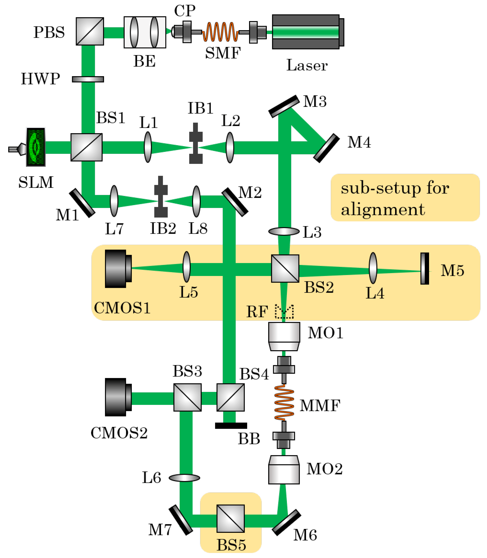
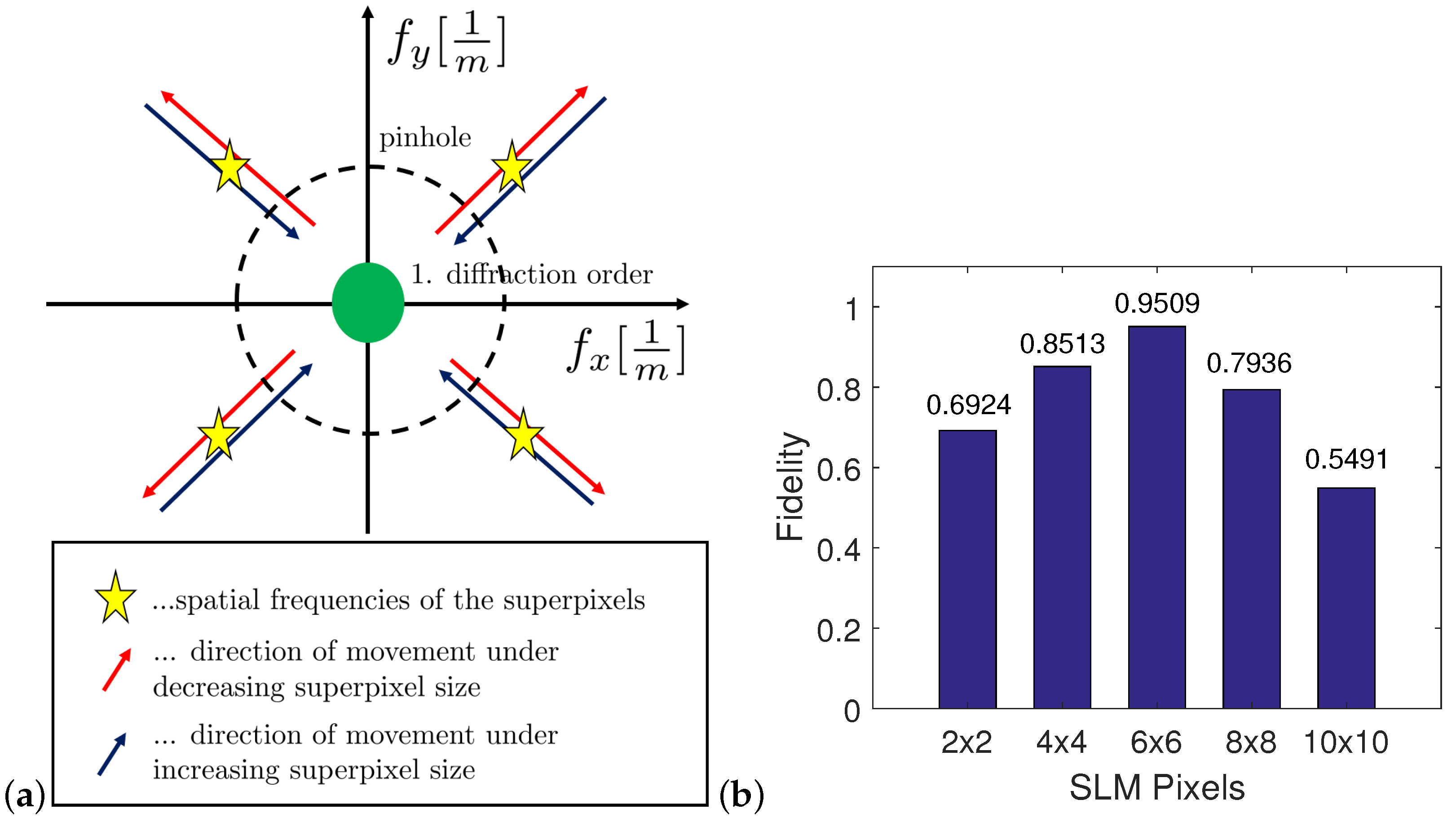
• Spatial filtering of the modulated light field
  In Section 2.1, it is explained that the derived superpixel distribution needs to be superimposed with a diffraction grating to filter the modulated signal that is located in the 1st diffraction order secluded from the center of the Fourier plane. It is necessary that the filtered signal (first diffraction order) is located on the optical axis to avoid unwanted optical aberrations, which can be achieved by tilting the SLM plane. After conduction, the passed light from IB in Figure 2 propagates through the center of L2.
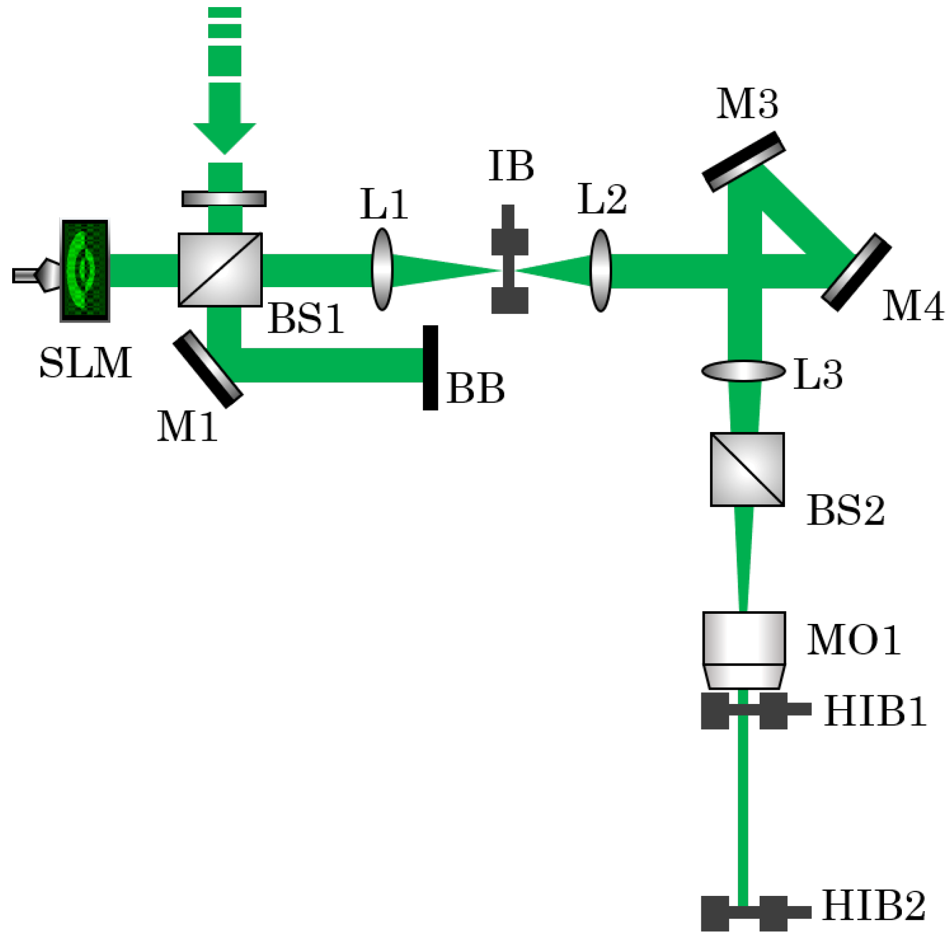
• Guiding the laser beam through microscope objective 1 (MO1)
  The utilized subsetup for aligning the laser beam through MO1 is shown in Figure 6. After the IFFT executed by L2, the beam is guided along a desired hole line on the optical bench using two mirrors M3 and M4 and two pinholes (HIB1 and HIB2). Now, L3 can be positioned in the beam path, which should not disturb the beam direction. Finally, the microscope objective can be positioned. In general, microscope objectives magnify small alignment deviations and therefore it is advisable to mount MO1 on a stage with μm precision. Eventually, the beam should propagate through HIB1 and HIB2 after every component was set in the path.
  Furthermore, it is mandatory for a proper mode excitation, that the IFFT with L2 and the telescope involving L3 and MO1 is performing correctly. This depends on the correct distances between the optical components and can be verified by modulating an image with the SLM. In this case, an axicon was used as a target test field. After propagation through the setup, the image behind MO1 can be monitored with a screen. On the screen, the phase boundaries should completely disappear.
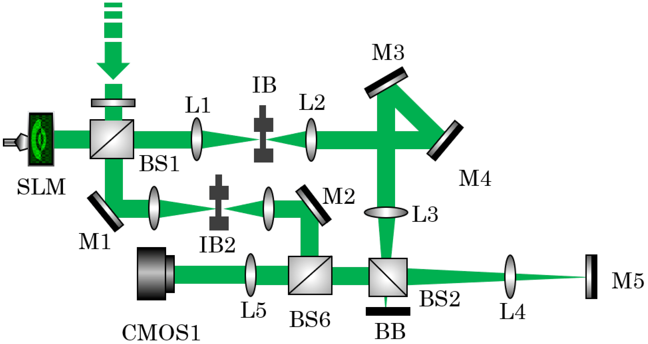
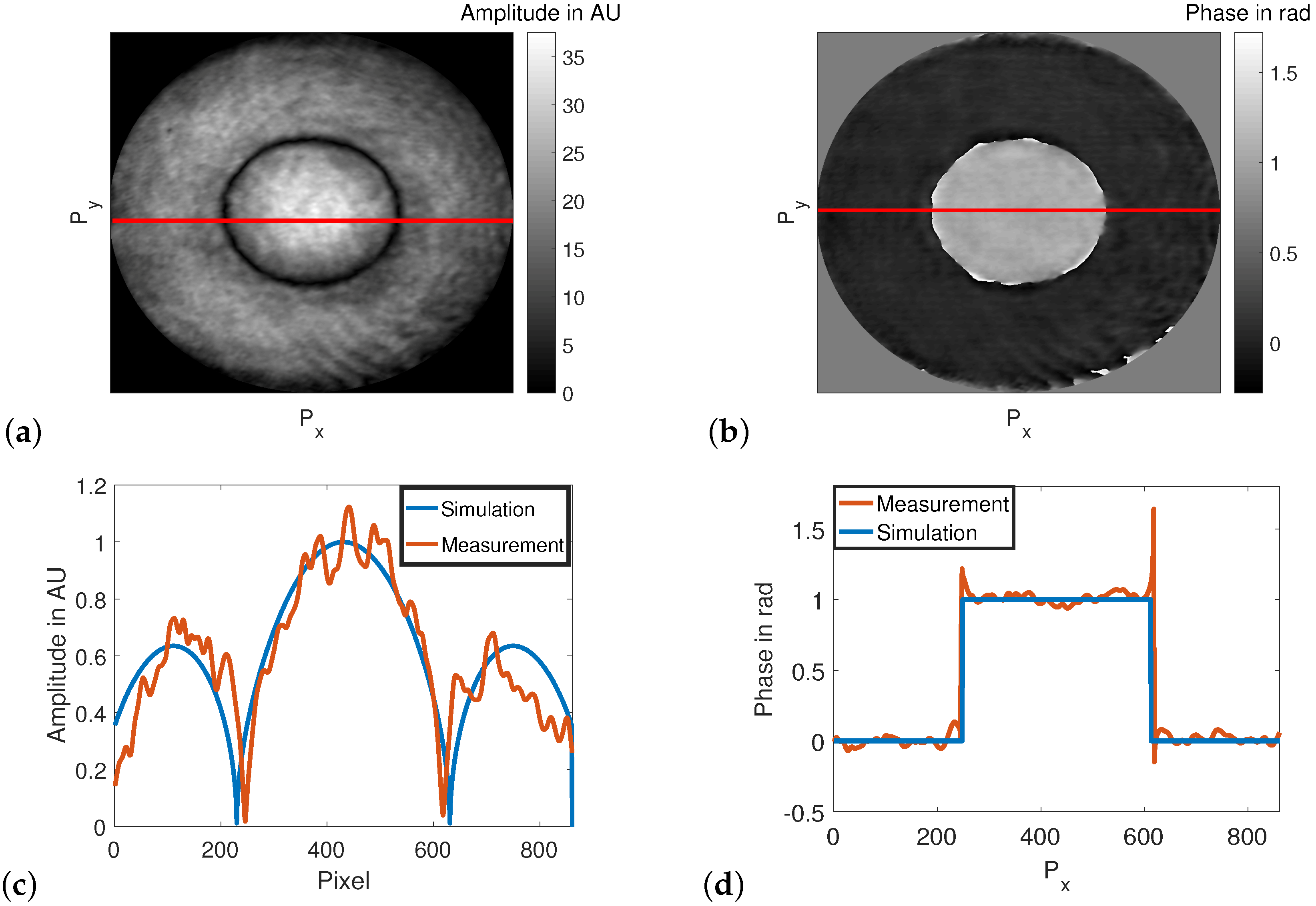
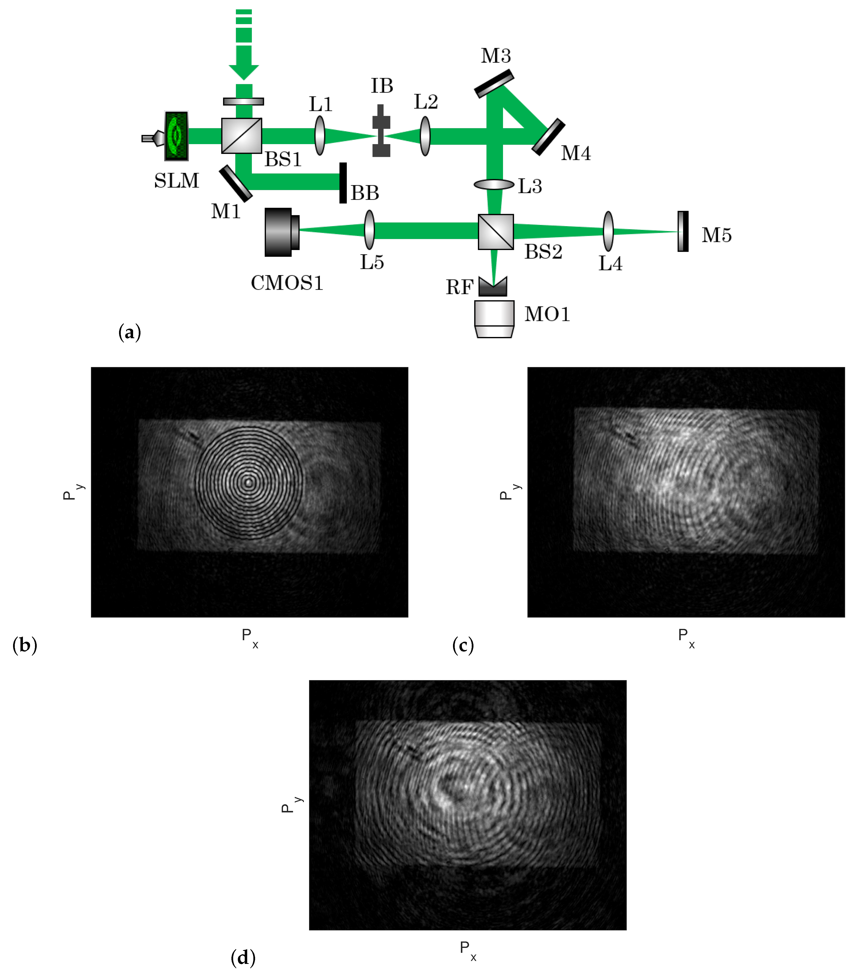
• Parallel imaging of the SLM plane to MO1
  For a proper mode excitation, the SLM plane has to be imaged onto to the input fiber facet. Deviating incident angles could lead to inappropriate mode excitation and should be neglected. Therefore, a non-invasive method to verify a parallel imaging of the mentioned planes was developed. The utilized sub-setup is shown in Figure 7a. The beam propagating through MO1 is split into a second path by BS2, propagates through L4 and is reflected by an auxiliary mirror M5, so that the reflected light is imaged on CMOS1 by another telescope involving L4 and L5. At first, the correct distances between the optical components should be ensured to provide a sharp image of the SLM plane on CMOS1. This was verified by modulating an axicon with the SLM once more. The captured intensity image of the axicon under proper conditions is shown in Figure 7b, where the boundary lines are of minimum thickness. Afterwards, by displaying the sheer diffraction grating on the SLM, the pure modulator plane is imaged on CMOS1 (see Figure 7c). Now, a retro reflector without beam displacement has to be placed in front of MO1 as shown in Figure 7a. Perpendicular alignment of the optical components causes concentric interference rings on CMOS1, as shown in Figure 7d.
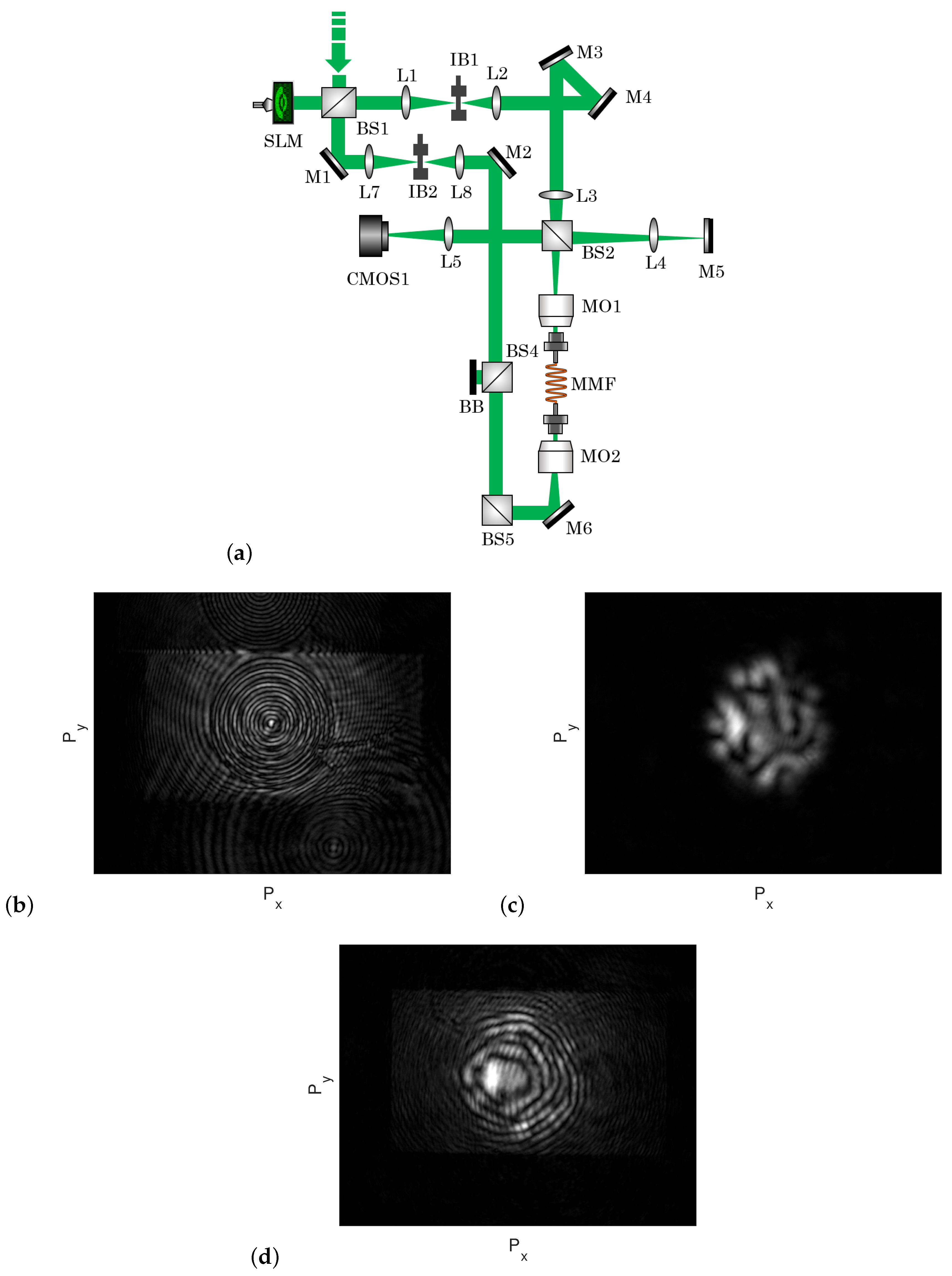
• Alignment of the MMF
  With the use of the auxiliary sub-setup introduced in step 3, the MMF can be aligned and a parallel imaging of the SLM plane to the input fiber facet plane is ensured. In the first instance, the MMF has to be set in its place of destination, as shown in Figure 8a. In the next step, light has to be coupled into the fiber at the actual output by using the reference beam. For the alignment, M2, BS5 and M6 can be tilted as desired. The light leaving the fiber input has to be captured with MO1 without moving MO1. This means that only the MMF can be aligned, so that light propagates through MO1 and is captured with CMOS1. In order to find the proper distance between MMF and MO1, the reference beam has to be blocked and an axicon is displayed once more. The back reflecting light from the input fiber facet is now imaged on CMOS1. As introduced in step 3, the MMF has to be moved until the boundary lines of the axicon are at a minimum thickness, as shown in Figure 8b. Now, the input fiber facet is located in the focal plane of MO1. By coupling the reference beam into the actual fiber output once more, a sharp image of the fiber input facet on CMOS1 can be seen, as shown in Figure 8c. Eventually, if the sheer diffraction grating is displayed on the SLM and the back reflected light from the input fiber facet interferes with the reflection from M5, concentric interference rings appear on CMOS1, as shown in Figure 8d.

2.3. Holographic Decomposition of Light into the Fiber’s Mode Domain

DH is one possible approach to extract amplitude and phase from an electromagnetic wave using a CMOS digital camera [26]. Applying this technique to the presented experimental setup, the fiber output light field can be measured and analyzed. Therefore, the MMF output signal is superimposed with the reference beam on CMOS2, as shown in Figure 1. The resulting hologram is captured with the camera and numerically reconstructed with the angular spectrum method [27].

In order to receive a quantitative phase measurement, the raw phase data from the measurement has to be relieved from several errors. These unwanted systematic parts of the measured phase data are due to wrapping errors, optical aberrations, phase offsets, MMF surface irregularities or dust on optical components. One approach to determine these error terms is to capture a reference hologram to identify a reference phase distribution, which can be set against the experimental results. In Section 3, it is explained how this is conducted during the TM acquisition.

For acquiring a fiber’s TM, the holographically measured complex light field has to be decomposed into the fiber’s mode domain. Since Maxwell’s equations are linear differential equations, the light guidance of an arbitrary input field ${\underline{E}}_{\mathrm{input}}$ in an MMF can be modeled as a linear sequence approach, where the orthogonal base functions are the complex spatial distributions of the supported fiber modes ${\underline{E}}_n$ [28]. The proportion of every mode to ${\underline{E}}_{\mathrm{input}}$ is determined by their individual weight $a_n$:

$${\underline{E}}_{\mathrm{input}}=\sum _{n=1}^N{a}_n{\underline{E}}_n=a_1{\underline{E}}_1+a_2{\underline{E}}_2+\dots +a_N{\underline{E}}_N.$$

(3)

Likewise, the measured field at the fiber output ${\underline{E}}_{\mathrm{obtained}}$ consisting of the measured amplitude $\left|A\right|$ and phase $\varphi$ distributions,

$${\underline{E}}_{\mathrm{obtained}}=\left|A\right|·e^{i\varphi },$$

(4)

needs to be analyzed considering the supported fiber modes ${\underline{E}}_n$ from the same mode domain:

$${\underline{E}}_{\mathrm{obtained}}=\sum _{n=1}^N{c}_n{\underline{E}}_n=c_1{\underline{E}}_1+c_2{\underline{E}}_2+\dots +c_N{\underline{E}}_N.$$

(5)

The coefficients $c_n$ determine the weight of the individual modes in the measured light field. In order to identify the coefficient of every mode in a measured light field, a linear system of equations is derived by multiplying the complex conjugate base functions ${\underline{E}}_1^{\ast }$, ${\underline{E}}_2^{\ast }$, …, and integrate over the whole space, named R. The integration is approximated by a two-dimensional sum, thus the camera captures a pixelated image:

$$\begin{array}{cc}\hfill \sum _R{\underline{E}}_{\mathrm{obtained}}{\underline{E}}_1^{\ast }& =c_1\sum _R{\underline{E}}_1{\underline{E}}_1^{\ast }+c_2\sum _R{\underline{E}}_2{\underline{E}}_1^{\ast }+\dots +c_N\sum _R{\underline{E}}_N{\underline{E}}_1^{\ast }\hfill \\ \hfill \sum _R{\underline{E}}_{\mathrm{obtained}}{\underline{E}}_2^{\ast }& =c_1\sum _R{\underline{E}}_1{\underline{E}}_2^{\ast }+c_2\sum _R{\underline{E}}_2{\underline{E}}_2^{\ast }+\dots +c_N\sum _R{\underline{E}}_N{\underline{E}}_2^{\ast }\hfill \\ \hfill \dots & =\dots \hfill \\ \hfill \sum _R{\underline{E}}_{\mathrm{obtained}}{\underline{E}}_N^{\ast }& =c_1\sum _R{\underline{E}}_1{\underline{E}}_N^{\ast }+c_2\sum _R{\underline{E}}_2{\underline{E}}_N^{\ast }+\dots +c_N\sum _R{\underline{E}}_N{\underline{E}}_N^{\ast }.\hfill \end{array}$$

(6)

The solution of this system becomes much easier due to the fact that the base functions are orthogonal to each other hence:

$$\sum _R{\underline{E}}_n{\underline{E}}_m^{\ast }=\left\{\begin{array}{cc}0\hfill & \mathrm{for}n\ne m\hfill \\ K_n\hfill & \mathrm{for}n=m\hfill \end{array}\right.$$

(7)

Therefore, the right hand side of every row n of the system (6) disappears, except the item $c_n{K}_n$ and so, the coefficients can be calculated by

$$c_n=\frac{1}{K_n}\sum _R{\underline{E}}_{\mathrm{obtained}}{\underline{E}}_n^{\ast }.$$

(8)

If Equation (8) is computed for every mode from the N-dimensional mode domain, the measured distribution ${\underline{E}}_{\mathrm{obtained}}$ is decomposed into the fiber’s mode domain by single-shot.

3. Acquisition of the Fiber’s Transmission Matrix

In the previous section, the experimental principles required for the direct TM acquisition were introduced. It is required to excite every mode of the supported fiber modes sequentially and directly without the need to use a conversion matrix as done in [11] or [12]. Selective mode excitations are especially beneficial for prospective information-technical applications, however the experimental work appears more challenging. The actual procedure of the TM acquisition is based on the work from [12]. To verify the developed technique with the experimental setup from Figure 1, a TM acquisition at an approximately 1 cm long piece of step-index MMF is presented. MMFs at this size have a weakly developed mode scrambling property [11]; thus, an acquired TM corresponds strongly to a diagonal matrix. This characteristic is used to provide a proof-of-principle of the presented system.

After the complex spatial mode functions from every supported fiber mode have been calculated and translated into a superpixel distribution, a reference phase distribution for the holographic-based decomposition method introduced in Section 2.3 is obtained. In order to measure systematic aberrations, it is necessary to let the object beam, which should be as unmodulated as possible, propagate through the optical setup to measure all the aberrations that act on the object beam. Since the errors, which have to be compensated, are located behind the MMF output, an unmodulated object beam at the fiber output needs to be generated. Due to the weakly developed scrambling at MMFs of approximately 1 cm length, the $L{P}_{01}$ mode is excited at the fiber input. The light that propagated through the MMF appears with a sufficiently homogeneous phase distribution at the MMF output and can be obtained holographically at CMOS2. The reconstructed amplitude and phase distributions are shown in Figure 9. Now, the correction can be conducted by calculating ${\varphi }_{\mathrm{corrected}}={\varphi }_{\mathrm{measured}}-{\varphi }_{\mathrm{Ref}}$.

With access to a quantitative phase measurement, the TM acquisition can be executed. The fiber under study supports $N=$ 110 fiber modes considering [28], where N is calculated by:

$$N\approx \frac{1}{2}·{\left(a·\frac{2\pi }{{\lambda }_0}·\mathrm{NA}\right)}^2,$$

(9)

with a being the MMF core radius. The fiber specifications are listed in

Table 1. Specifications of the used MMF.

Specification	Value
$NA$	$0.1\pm 0.015$
a	$(25\pm 3)$ μm
${\lambda }_0$	532 nm

.

Hence, the expected TM is of dimensions $110\times 110$, which means that for each polarization direction a $55\times 55$ TM can be acquired. Now, every mode contained in the fiber’s mode domain has to be excited sequentially at the fiber input. The propagated light fields are superimposed with the reference beam on CMOS2, where holograms are captured. The holograms are reconstructed numerically with the angular spectrum method. Afterwards, the decomposition has to be executed for every shot. The resulting coefficients from the i-th mode of the mode domain are stored in the i-th row of the TM. Within the introduced experiment, the TM shown in Figure 10 was measured. Both the input and output vectors with the determined coefficients are arranged following the mode group manner presented in [7]. One result was that every ${\mathrm{LP}}_{\mathrm{lm}}$ mode belongs to a mode group given by $2m+l-1$. Modes inside a group mix heavily with each other.

4. Discussion

The introduced superpixel method was implemented in the presented optical setup. This technique enables arbitrary complex modulation with one phase-only SLM. Therefore, a high-fidelity mode generation is possible. Hence, the supported fiber modes can be directly excited at the fiber input. A theoretical maximum of the presented technique of $F_{\mathrm{theoretical}}=0.9943$ was derived. During the experiment, a value of $F=0.9509$ could be achieved, which corresponds to $95.6\%$ of $F_{\mathrm{theoretical}}$. The main part of occurring deviations in the simulation can be explained with the overlaying diffraction grating on the superpixel pattern to reduce the influences of undesired polarizations of light or unmodulated light. This leads to a trade-off between the size of the superpixel and the grating. The selective mode excitation is followed by a challenging alignment procedure, which could be managed by developing specific adjustment methods. A DH-based decomposition technique that is used to analyze the propagated light with respect to containing fiber modes was introduced. Hence, one row of the acquired TM can be obtained in a single-shot and reduces the measurement effort by a factor of 4 in relation to phase-shifting-based acquisition methods or factor N in relation to correlation filter methods. Presently, the bottle neck regarding the TM acquisition time is the SLM’s frame rate (best performance at approximately 20 Hz). Eventually, a TM measurement of an approximately 1 cm long piece of MMF was conducted. At these propagation distances, mode coupling effects are weakly developed, so that a TM resembles a diagonal matrix so long as laboratory conditions are constantly complied. The major power of the resulting TM, which is shown in Figure 10, is clearly distributed over the diagonal elements. Hence, a proof of the presented principle could be accomplished. However, TM entries off the diagonal have a value significantly greater than background noise and need to be discussed. By using a piece of MMF, which has a length of approximately 1 cm, it was intended to reduce the scattering property of the investigated sample. Yet, the utilized laser with ${\lambda }_0=$ 532 nm propagates with approximately 20,000 waves through the waveguide, which is still enough to come upon manufacturing imperfections. In Table 1, the fiber properties with the given tolerances are listed. Both the core diameter and the NA have a tolerance of more than 10%—these are imperfect conditions. In [11], the authors obtained similar results: the simulated phase distribution after propagation through an approximately 10 cm piece of step-index MMF did not fit the experimental results until they superimposed the ideal refractive index profile with Zernike polynomials. As a consequence, the person who works with MMFs should address manufacturing imperfections. The presented results open the door to fast TM acquisition procedures of highly moded MMFs using MDM. In such procedures, the amplitude and phase relations are determined to understand the mode scrambling processes inside the MMF affecting the TM.

5. Conclusions

An optical setup in order to excite N-supported fiber modes of a step-index MMF with a phase-only SLM using superpixels was investigated. With a novel decomposition method based on digital holography, the TM of a MMF is measured with only N measurements. This paves the way for prospective rapid TM measurements. The TM of MMF provides important channel information for the implementation of Mode Division Multiplexing, which is based on Multiple Input Multiple Output (MIMO). As a perspective, MIMO can be used to increase the secure goodput of the data transfer based on physical layer security.

References

1. Papadopoulos, I.N.; Farahi, S.; Moser, C.; Psaltis, D. Focusing and scanning light through a multimode optical fiber using digital phase conjugation. Opt. Express 2012, 20, 10583–10590. [Google Scholar] [CrossRef] [PubMed]
2. Haufe, D.; Koukourakis, N.; Büttner, L.; Czarske, J. Transmission of multiple signals through an optical fiber using wavefront shaping. J. Vis. Exp. 2017, 121, e55407. [Google Scholar] [CrossRef] [PubMed]
3. Czarske, J.W.; Haufe, D.; Koukourakis, N.; Büttner, L. Transmission of independent signals through a multimode fiber using digital optical phase conjugation. Opt. Express 2016, 24, 15128–15136. [Google Scholar] [CrossRef] [PubMed]
4. Florentin, R.; Karmene, V.; Benoist, J.; Desfarges-Berthelemot, A.; Pagnoux, D.; Barthélémy, A.; Huignard, J.P. Shaping the light amplified in a multimode fiber. Light Sci. Appl. 2017, 6, e16208. [Google Scholar] [CrossRef] [PubMed]
5. Berdagué, S.; Facq, P. Mode division multiplexing in optical fibers. Appl. Opt. 1982, 21, 1950–1955. [Google Scholar] [CrossRef] [PubMed]
6. Ryf, R.; Fontaine, N.K.; Chen, H.; Guan, B.; Huang, B.; Esmaeelpour, M.; Gnauck, A.H.; Randel, S.; Yoo, S.J.B.; Koonen, A.M.J.; et al. Mode-multiplexed transmission over conventional graded-index multimode fibers. Opt. Express 2015, 23, 235–246. [Google Scholar] [CrossRef] [PubMed] [Green Version]
7. Carpenter, J.; Thomsen, B.C.; Wilkinson, T.D. Degenerate Mode-Group Division Multiplexing. J. Lightw. Technol. 2012, 30, 3946–3952. [Google Scholar] [CrossRef]
8. Richardson, D.J.; Fini, J.M.; Nelson, L.E. Space-division multiplexing in optical fibres. Nat. Photonics 2013, 7, 354–362. [Google Scholar] [CrossRef] [Green Version]
9. Jorswieck, E.; Wolf, A.; Gerbracht, S. Secrecy on the Physical Layer in Wireless Networks. In Trends in Telecommunications Technologies; INTECH: Boston, MA, USA, 2010; pp. 413–435. [Google Scholar]
10. Popoff, S.M.; Lerosey, G.; Carminati, R.; Fink, M.; Boccara, A.C.; Gigan, S. Measuring the Transmission Matrix in Optics: An Approach to the Study and Control of Light Propagation in Disordered Media. Phys. Rev. Lett. 2010, 104, 100601–100605. [Google Scholar] [CrossRef] [PubMed]
11. Plöschner, M.; Tyc, T.; Čižmár, T. Seeing through chaos in multimode fibres. Nat. Photonics 2015, 9, 529–535. [Google Scholar] [CrossRef]
12. Gu, R.Y.; Mahalati, R.N.; Kahn, J.M. Design of flexible multi-mode fiber endoscope. Opt. Express 2015, 23, 26905–26918. [Google Scholar] [CrossRef] [PubMed]
13. Flamm, D.; Schulze, C.; Naidoo, D.; Schröter, S.; Forbes, A.; Duparré, M. All-Digital Holographic Tool for Mode Excitation and Analysis in Optical Fibers. J. Lightw. Technol. 2013, 31, 1023–1032. [Google Scholar] [CrossRef]
14. N’Gom, M.; Norris, T.B.; Michielssen, E.; Nadakuditi, R.R. Mode control in a multimode fiber through acquiring its transmission matrix from a reference-less optical system. Opt. Lett. 2018, 43, 419–422. [Google Scholar] [CrossRef] [Green Version]
15. Koukourakis, N.; Fregin, B.; König, J.; Büttner, L.; Czarske, J.W. Wavefront shaping for imaging-based flow velocity measurements through distortions using a Fresnel guide star. Opt. Express 2016, 24, 22074–22087. [Google Scholar] [CrossRef] [PubMed]
16. Kuschmierz, R.; Scharf, E.; Koukourakis, N.; Czarske, J.W. Self-calibration of lensless holographic endoscope using programmable guide stars. Opt. Lett. 2018, 43, 2997–3000. [Google Scholar] [CrossRef] [PubMed]
17. Tzang, O.; Caravaca-Aguirre, A.M.; Wagner, K.; Piestun, R. Adaptive wavefront shaping for controlling nonlinear multimode interactions in optical fibres. Nat. Photonics 2018, 12, 368–374. [Google Scholar] [CrossRef]
18. Schmieder, F.; Klapper, S.D.; Koukourakis, N.; Busskamp, V.; Czarske, J.W. Optogenetic Stimulation of Human Neural Networks Using Fast Ferroelectric Spatial Light Modulator—Based Holographic Illumination. Appl. Sci. 2018, 8, 1180. [Google Scholar] [CrossRef]
19. Van Putten, E.G.; Vellekoop, I.M.; Mosk, A.P. Spatial amplitude and phase modulation using commercial twisted nematic LCDs. Appl. Opt. 2008, 47, 2076–2081. [Google Scholar] [CrossRef]
20. Goorden, S.A.; Bertolotti, J.; Mosk, A.P. Superpixel-based spatial amplitude and phase modulation using a digital micromirror device. Opt. Express 2014, 22, 17999–18009. [Google Scholar] [CrossRef]
21. Forbes, A.; Dudley, A.; McLaren, M. Creation and detection of optical modes with spatial light modulators. Adv. Opt. Photonics 2016, 8, 200–227. [Google Scholar] [CrossRef]
22. Chu, D.C.; Goodman, J.W. Spectrum Shaping with Parity Sequences. Appl. Opt. 1972, 11, 1716–1724. [Google Scholar] [CrossRef] [PubMed]
23. Brüning, R.; Flamm, D.; Ngcobo, S.S.; Forbes, A.; Duparré, M. Rapid measurement of the fiber’s transmission matrix. Proc. SPIE 2015, 9389, 93890N. [Google Scholar]
24. García-Márquez, J.; López, V.; González-Vega, A.; Noé, E. minimization in an LCoS spatial light modulator. Opt. Express 2012, 20, 8431–8441. [Google Scholar] [CrossRef] [PubMed]
25. Jang, M.; Ruan, H.; Zhou, H.; Judkewitz, B.; Yang, C. Method for auto-alignment of digital optical phase conjugation systems based on digital propagation. Opt. Express 2014, 22, 14054–14071. [Google Scholar] [CrossRef] [PubMed] [Green Version]
26. Schnars, U.; Jüptner, W. Direct recording of holograms by a CCD target and numerical reconstruction. Appl. Opt. 1994, 33, 179–181. [Google Scholar] [CrossRef] [PubMed]
27. Koukourakis, N.; Abdelwahab, T.; Li, M.Y.; Höpfner, H.; Lai, Y.W.; Darakis, E.; Brenner, C.; Gerhardt, N.C.; Hofmann, M.R. Photorefractive two-wave mixing for image amplification in digital holography. Opt. Express 2011, 19, 22004–22023. [Google Scholar] [CrossRef] [PubMed]
28. Gloge, D. Weakly Guiding Fibers. Appl. Opt. 1971, 10, 2252–2258. [Google Scholar] [CrossRef] [PubMed]
Figure 1. Experimental scheme. The laser beam is coupled to a single mode fiber (SMF), collimated by a collimation package (CP) and widened by a beam expander (BE). A polarizing beam splitter (PBS) and a half-wave plate (HWP) filter the laser beam at a linear polarization, matching the SLM required modulation polarization. Beamsplitter 1(BS1) splits the laser beam into reference and object beam, which is reflected at the SLM plane after being modulated by the SLM pixels. Lens 1 (L1) executes an optical Fourier Transform (FFT) to the modulated laser beam, so a pinhole (IB) filters the first diffraction order in the Fourier plane. L2 executes an optical inverse Fourier Transform (IFFT). L3 and microscope objective 1 (MO1) image the filtered beam onto the fiber facet of the MMF. To yield excitation conditions as precise as possible, the incidence angle of the beam is tuned by two mirrors M3 and M4. The light, that is propagated through the MMF is imaged on camera 2 (CMOS2) with a telescope composed of MO2 and L6. The hologram, which is generated by the interference between the light field that exits the MMF and the reference beam is captured by CMOS2. The reference beam is cleaned up with L7, IB2 and L8. Afterwards, the reference beam is directed onto CMOS2 with M1, M2 and BS4. For proper alignment, the sub-setups in the yellow boxes are used and are explained in detail in Section 2.2. Laser: 532 nm Laser Quantum torus; SMF: THORLABS P3-460B-FC-5; CP: collimator PAF2-A4A; BE: beam expander GBE10-A 10x; HWP: half-wave plate; SLM: HOLOEYE Pluto-2; M1-M6: protected silver mirrors PF10-03-P01; BS1-BS5: 50:50 beam splitter cubes BS013; PBS: polarizing beam splitter cubes PBS251; IB1-2: pinholes D36S; L1-L8: lenses f1 = 250 mm, f2 = 60 mm, f3 = 160 mm, f4 = 80 mm, f5 = 180 mm, f6 = 300 mm, f7 = 60 mm, f8 = 160 mm; MO1: 80x Mitutoyo Plan Apo SL; MO2: Olympus PLN 40x; MMF: THORLABS FG025LJA; BB: beam block; CMOS1 and CMOS2: IDS UI348xLE-M.
Applsci 09 00195 g001
Figure 2. Optical setup for investigation of the superpixel method. This is a sub-setup from the setup shown in Figure 1. For this procedure, BS6 is used to generate a hologram on CMOS1.
Applsci 09 00195 g002
Figure 3. Superposition of complex pointers. (a) Generation of an arbitrary complex pointer by superimposing two different complex pointers. (b) Generation of a mode data entry with two symmetrically displaced unit pointers for the superpixel map being displayed on a phase-only SLM. (c) Resulting superpixel that represents the desired complex pointer C ( j ω ). 3 × 3 SLM-Pixel form one subpixel.
Applsci 09 00195 g003
Figure 4. Experimental results from a superpixel-based modulation of a light field. The measured light field is compared with the target LP 02 mode distribution. (a) Amplitude distribution of the measured light field. The red line indicates the analyzed profile route shown in c. (b) Phase distribution of the measured light field. The red line indicates the analyzed profile route shown in d. (c) Amplitude profile of the measured light field compared with the target profile. (d) Phase profile of the measured light field compared with the target profile.
Applsci 09 00195 g004
Figure 5. Investigation of superpixel influences on spatial frequencies and resulting fidelity. (a) Scheme to illustrate the dependency between spatial frequency movement and superpixel size. (b) Measured fidelity of generating a L P 02 mode by varying superpixel size.
Applsci 09 00195 g005
Figure 6. Optical setup to align the microscope objective. This is a sub-setup from the setup shown in Figure 1.
Applsci 09 00195 g006
Figure 7. An auxiliary sub-setup helps to image the SLM plane to the input fiber facet plane. At first, the auxiliary path with L4 and M5 needs to be set properly: (a) sub-setup from Figure 1; (b) sharp image from an axicon reflected by the auxiliary mirror M5 and captured with CMOS1; (c) sharp image of the modulator plane reflected from M5 and captured with CMOS1. The SLM displays the sheer diffraction grating; (d) after the retro reflector is set, concentric interference rings appear on CMOS1.
Applsci 09 00195 g007
Figure 8. For the alignment of the MMF, the reference beam is coupled to the actual output of the MMF and the image from the input fiber facet on CMOS1 is analyzed: (a) sub-setup from Figure 1; (b) sharp image from an axicon reflected by the input fiber facet and captured with CMOS1; (c) sharp image of the input fiber facet and captured with CMOS1; (d) after the MMF is aligned properly, concentric interference rings appear on CMOS1 if the back reflected light from the input fiber facet interferes with the reflected light from M5. The sheer diffraction grating is displayed on the SLM.
Applsci 09 00195 g008
Figure 9. Reconstruction of the reference hologram captured with CMOS2 by exciting an L P 01 mode at the fiber input: (a) reconstructed phase distribution; (b) reconstructed amplitude distribution.
Applsci 09 00195 g009
Figure 10. Measured TM of one linear polarization direction of a MMF. During the experiment, constant laboratory conditions were guaranteed.
Applsci 09 00195 g010