Local, Story, and Global Ductility Evaluation for Complex 2D Steel Buildings: Pushover and Dynamic Analysis

Abstract

A numerical investigation regarding ductility evaluation of steel buildings with moment resisting steel frames is conducted. Bending (µ_Lϕ) and tension (µ_Lδ) local ductilities as well as story (µ_S) and global ductilities are studied. Global ductility is calculated as the mean values of story ductilities (µ_GS) and as the ratio of the maximum inelastic to yielding top displacements (µ_Gt). The ductility capacity is associated to drifts of about 5%. Ductility values significantly may vary with the strong motion, ductility definition, structural element, story number, type of analysis, and model. µ_Lϕ is much larger for beams than for columns. Even though the demands of µ_Lδ are considered an important issue they are less relevant than µ_Lϕ. µ_S is much smaller than µ_Lϕ for beams. µ_GS for dynamic analysis give reasonable values, but µ_Gt does not. µ_Lϕ, µ_S and µ_GS obtained from pushover are larger than those obtained from dynamic analysis and unlike the case of dynamic analysis, µ_Lϕ tend to increase with the story number showing an opposite trend. Considering that: µ_Gt for dynamic analysis results in unreasonable values, pushover analysis does not consider energy dissipation, the strong column–weak beam (SCWB) concept was followed in the model designs, and µ_Lδ is not relevant in framed steel buildings, the ratio (R_LG) of global to local ductility capacity is calculated as the ratio of µ_GS to µ_Lϕ of beams, for dynamic analysis. A value of 1/3 is proposed. Thus, if bending local ductility capacity is stated as the basis for the design, the global ductility capacity can be easily estimated.

1. Introduction

The seismic behavior of a building under the action of a strong motion represents a very complicated phenomenon, particularly when the building is deformed into the inelastic range. In spite of this most of building codes around the world permit the use of simple elastic procedures to determine the seismic demands on steel buildings either for small or large deformations. Due to their relatively simplicity in their application, simplified methods like the Static Equivalent Lateral Force (SELF) procedure, are broadly used. For example, The International Building Code (IBC) [1], The National Building Code of Canada (NBCC) [2], The Mexico Federal District Code (MFDC) [3], and The Eurocode 8 (EC) [4], permit the use of the mentioned procedure for regular buildings with relatively short periods (low- and medium-rise). FEMA-273 and ATC-40 also permit to use nonlinear static procedure or pushover analysis. In the procedure, static analysis of the buildings under the action of equivalent lateral forces, which are related to the properties of the structure and the seismicity of the region, provides the design forces; then a serviceability revision is performed. Thus, it can be said that conventional seismic design considered in many seismic codes is essentially force-based with a final check on displacements.

In the above mentioned procedure, the ductility parameter (µ) plays an important role in the determination of the design seismic forces of building structural systems, it represents the capacity of a structure to dissipate energy, allowing for a reduction of the elastic strength demands; the larger the ductility, the smaller the design seismic forces. It is particularly important for steel structures since there are many sources of ductility and of energy dissipation. However, there is not unanimity on the profession on how to define it; it is argued that this parameter is constantly used in the profession in an indirect way to estimate the building seismic design forces, but there is no engineering definition of it in our specifications or unanimity on the profession on how to define it [5,6]. In fact, the magnitude of the reduction of the elastic design seismic forces directly depends on the force reduction factor (R), which significant depends on an associated parameter called ductility reduction factor (R_µ) [7,8]. The estimation of these parameters represents one of the most controversial issues in the SELF procedure.

In IBC the reduction factor is called ‘response modification factor’ (R); it is stated that it depends on many parameters including the ductility capacity and inelastic performance of structural material. In NBCC the reduction parameter is called ‘force modification factor’ (R_d), where it is explicitly stated that it depends on the ductility capacity and materials as well as on the structural overstrength. In MFDC this parameter is called ‘seismic reduction factor’ (Q′) which depends on the structural material, the structural system and detailing. In EC the factor is called ‘seismic reduction factor’ (q′) and depends on an overstrength factor and on factors which in turn depends on structural materials and the structural system. It is implicitly assumed in these codes that ductility represents the capacity of the structure to dissipate energy.

It is concluded that, it is essential to establish a measure of ductility. In this regard, the various types of ductility involved in a building must be considered [9]; local ductility must be differentiated from story or from global ductility. For the case of steel buildings, local ductility may be associated to the rotational capacity of a member under bending or to the longitudinal deformation capacity of a member under tension. Story ductility is essentially associated to the relative story displacements while global ductility is normally expressed in terms of story ductility or in terms of the absolute displacements of the roof. It is generally accepted than the local ductility is larger than story ductility, which in turn is larger than global ductility.

It must be noted that ductility demand is different from ductility capacity. For example, for the case of a particular story, story ductility demand is the ratio of the maximum interstory lateral displacement of a structure during the application of the seismic loading to the corresponding displacement when first yielding occurs at any member of the story, while ductility capacity is the ratio of the maximum permissible inelastic lateral displacement to the displacement when first yield occurs. Ductility capacity is usually obtained from experimental results of individual members (local ductility). Therefore, it is important to relate it to the story or to the overall structural ductility (global ductility). Theoretically, ductility capacity should be reached when a collapse mechanism develops in the structure. To obtain this, it needs to be guaranteed that plastic moments are reached at positions of maximum moments before failure due to instability, namely local buckling or lateral torsional buckling, in a member or in a connection occurs. Moreover, local ductility cannot be exceeded; otherwise, the ductility corresponding to the collapse mechanism will not be the ductility capacity. For that reason, some researchers [10] suggest using local ductility as the basis for design because there are numerous laboratory studies on ductility for members. In this regard, as stated above, some relationships need to be established between local, story and global ductility.

The central objective of this paper is to evaluate the ductility parameter for steel buildings with typical welded moment-resisting frames. Different types of local ductility as well as story and global ductility are calculated according to both, nonlinear dynamic analysis and nonlinear static analysis (pushover). The relationship between local and global ductility is calculated. Due to the advancements in the computer technology, the computational capabilities have significantly increased in the recent years allowing us to estimate the nonlinear seismic response by modeling structures as complex MDOF systems with hundred and even thousands of degrees of freedoms and applying the seismic loadings in time domain as realistically as possible. Responses obtained in this way may represent the best estimate of the seismic responses. Then the values of ductility demands for the different definitions can be properly estimated.

2. Literature Review

Studying the µ parameter and the associated ductility reduction factor (R_μ for the case of the IBC code) of steel buildings has been an important research topic during the last decades. There have been a significant number of studies for single degree of freedom (SDOF) systems based on analytical and/or empirical observations and considerations. The R_μ factor was first introduced in ATC-3-06 [11] in the late 1970s. Other of the first investigations was conducted by Newmark and Hall [9]; they proposed a procedure to relate R_μ and µ by constructing the inelastic response spectra from the basic elastic design spectra. Hadjian [12] studied the reduction of the spectral accelerations to account for the inelastic behavior of structures. Miranda and Bertero [13] proposed simplified expressions to estimate the inelastic design spectra. Tiwari and Gupta [14] proposed a preliminary scaling model to estimate the ductility reduction factors of horizontal ground motions. Significant contributions regarding the evaluation of the ductility and ductility reduction parameters for SDOF systems can be found in other publications [15,16,17,18,19,20]. More recently Zhai et al. [21] investigated the strength reduction factor of SDOF systems with constant ductility performance subjected to the mainshock–aftershock sequence-type ground motions. Ghods et al. [22], by using the finite element method (FEM), investigated the forming of plastic hinges, distribution of stresses, and ductility and stiffness of steel systems composed of reinforced concrete column to steel beam connections.

There are also several studies regarding the evaluation of R (or R_µ) and µ factors for multi degree of freedom (MDOF) systems. Nassar and Krawinkler [23] studied the relationship between force reduction factors and ductility for simplified (three-story single-bay) MDOF systems. Santa-Ana and Miranda [24] studied the strength reductions factors for several steel frames modeled as plane MDOF systems. Moghaddam and Mohammadi [25] introduced a modification to the response modification factor and proposed an approach to evaluate the seismic strength and ductility demands of MDOF structures. Elnashai and Mwafy [26] investigated the relationship between the lateral capacity, the design force reduction factor, the ductility factor and the overstrength factor for reinforced-concrete buildings. Medina and Krawinkler [27] presented an evaluation on drift demands for regular moment resisting frame structures subjected to ordinary ground motions. In another study Medina and Krawinkler [28] studied the strength demands relevant for the seismic design of moment-resisting frames. Important results, regarding ductility, ductility reduction factor and other related parameters for structures modeled as MDOF systems can be found in some research reports and papers [29,30,31,32,33,34,35,36,37,38].

More recently Reyes-Salazar et al. [39], studied the ductility reduction factor for buildings with moment resisting steel frames (MRSF) which were modeled as complex MDOF systems, considering an intermediate level of inelastic structural deformation. Valenzuela-Beltran et al. [40] proposed a reliability-based criterion including two simplified mathematical expressions, which depends on the ductility of the structural system, to estimate strength amplification factors for buildings with asymmetric yielding. Fanaie and Shamlou [41] studied the seismic behavior, in terms of response modification factor and ductility factor, of mixed structures. Vuran and Aydınoğlu [42] developed simple capacity and ductility demand estimation tools for coupled core wall systems. Gómez-Martínez et al. [43] analytically studied the local and global ductility of wide-beam reinforced concrete moment resisting frames. Wang et al. [44] studied the seismic performances of steel braced truss-RC column hybrid structure. Liu et al. [45] developed a new response spectrum method by incorporating the ductility factor and strain rate into the conventional response spectrum method. Hashemi et al. [46] presented the results of studies on two important seismic parameters namely, ductility and response modification factor for moment resisting frames with concrete-filled steel tube columns. Kang and Mory [47] proposed simplified procedure to estimate the peak inter-story drift ratios of steel frames with hysteretic dampers for SDOF and MDOF systems where the energy dissipated by hysteretic behavior and the involved ductility were explicitly considered.

The abovementioned studies represent a significant contribution regarding the evaluation of ductility or force reduction factors, however, in most of them SDOF systems, plane shear buildings, or a limited level of inelastic deformation were considered. Therefore, they did not explicitly consider the inelastic behavior and energy dissipation of the structural elements existing in actual systems. It has been shown [48,49,50] that ductility demands as well as the ductility reduction factors depend on the amount of dissipated energy, which in turn depends on the plastic mechanism formed in the frames as well as on the loading, unloading and reloading process at plastic hinges. In addition, a limited level of inelastic deformation is not associated to the ductility capacity. Moreover, local ductility taking into account the maximum inelastic curvature and tensional elongations as well as relationship between local and global ductility, estimated by dynamic and pushover analysis, have not been considered.

3. Objectives

The central objective of this paper is to evaluate ductility demands of steel buildings; local, story and global ductility as well as relationship among them are considered. To this aim, the nonlinear seismic responses of low- and medium-rise steel building models with typical welded connections, idealized as complex plane MDOF systems, are calculated. The ductility values are compared with those resulting from pushover analysis. The specific objectives are:

(1)

Calculate local ductility for individual structural elements (beams and columns) associated to the maximum inelastic curvatures and axial elongations according to nonlinear seismic analysis. Several intensities of the strong motions are considered. The larger intensity of the earthquakes will correspond to a deformation state close to a structural collapse mechanism (maximum drifts of about 5%).

(2)

Calculate story and global ductility for the same cases above mentioned.

(3)

Compare the ductility values obtained from nonlinear dynamic analysis with those of pushover analysis.

(4)

Propose a relationship between local and global ductility.

4. Procedure and Structural Models

Two steel buildings, modeled as MDOF plane frames, and twenty strong seismic motions are used in the study. Local, story and global ductility, according to several definitions, are calculated. The strong motions are scaled down and up to get different levels of structural deformations. The maximum deformation level is very close to the formation of a collapse mechanism; therefore, it is associated to the ductility capacity. In some experimental studies it has been shown that moment resisting steel frames may undergo interstory displacements of up to 5% (and even larger) and still be able to vibrate in stable manner [51,52,53,54]. This is approximately the maximum deformation level considered in this study. Thus, the ductility values obtained for this deformation, according to the different definitions, are assumed to be the ductility capacity.

4.1. Steel Building Models

Several steel model buildings were designed, as part of the SAC (Structural Engineers of California, Applied Technology Council, and Consortium of Universities for Research in Earthquake Engineering) steel project [55], by three consulting firms. The buildings are supposed to satisfy all code requirements existed at the time of evaluation for the following three cities: Los Angeles [56], Seattle [56], and Boston [57]. The buildings were designed to be case studies to evaluate many aspects related to the seismic behavior of steel buildings with moment resisting frames [55]. Even though the three sets of buildings were used in the SAC project only the perimeter moment resisting frames (PMRF) of the 3- and 10-level buildings of the project, which are assumed to be located in the Los Angeles area, are considered in this study to address the issues discussed earlier. Isometric views for the 3- and 10-level buildings, which are referred hereafter as Models 1 and 2, respectively, are given in Figure 1 and Figure 2, where the PMRF (exterior) and the interior gravity frames are clearly identified. Sizes of structural elements, namely beams (horizontal) and columns (vertical), as reported, are given in

Table 1. Beam and columns sections for Models 1 and 2.

Model	Story	Columns		Girder
		Exterior	Interior
1	1/2	W14X257	W14X311	W33X118
	2/3	W14X257	W14X312	W30X116
	3/ROOF	W14X257	W14X313	W24X68
2	−1/1	W14X370	W14X500	W36X160
	1/2	W14X370	W14X500	W36X160
	2/3	W14X370	W14X500, W14X455	W36X160
	3/4	W14X370	W14X455	W36X135
	4/5	W14X370, W14X283	W14X455, W14X370	W36X135
	5/6	W14X283	W14X370	W36X135
	6/7	W14X283, W14X257	W14X370, W14X283	W36X135
	7/8	W14X257	W14X283	W30X99
	8/9	W14X257, W14X233	W14X283, W14X257	W27X84
	9/ROOF	W14X233	W14X257	W24X68

for the two models. The first three translational periods of the plane frames associated to lateral vibrations are 1.03 s, 0.30 s, and 0.15 s, for the 3-level model; the corresponding values for the 10-level model are 2.41 s. 0.89 s, and 0.5 s.

The building models are assumed to have typical welded connections. The structural members, which were modeled as one-dimensional beam-column elements, were designed following the strong column–weak beam (SCWB) concept. Each column is represented by one element and each girder by two elements, having a node at the mid-span. Each node is considered to have three degrees of freedom. The damping is considered to be 3% of critical damping. The RUAUMOKO Computer Program [58] is used for the time history nonlinear dynamic analysis. The frames are modeled as complex 2D MDOF systems. The Newmark constant average acceleration method together with the Newton–Raphson iteration scheme are used to solve the differential equation systems. For a given load increment convergence occurs (it is the iterative process is terminated) when the ratio of the incremental displacements at the current iteration to the current estimate of the displacements is small enough (about 0.00001). In addition lumped mass matrix, Rayleigh damping as well as large displacement effects, are considered in the nonlinear dynamics analysis; the time increment in the analysis was 0.01 s. The panel zone was considered to be rigid. Typical input data as ground accelerations, boundary conditions, node coordinates, as well as elastic and inelastic section properties are given or read within the Ruaumoko computer program environment. No strength degradation member, bilinear behavior with 5% of the initial stiffness in the second region and concentrated plasticity are assumed. The interaction axial load-bending moment is given by the yield interaction surface proposed by Chen and Atsuta [59].

It is worth mentioning that the numerical investigation was developed on the base of the above-described simplified FE models, where the mechanical, geometrical, and dynamics properties of structural elements are roughly, but efficiently, described. It has been shown [60,61,62,63] that this type of FE formulation results in a good approximation of the structural response in parametric studies like that presented in this paper, as long as it is provided a realistic modeling of the structure and of the cyclic load deformation characteristics of its structural elements.

4.2. Earthquake Loading

The responses of a structure excited by different strong motions, even when they are normalized with respect to the same response parameter, are expected to be different reflecting the influence of their different frequency content. Thus to get meaningful results, the models under consideration are excited by twenty strong motions in time domain. The characteristics of the records are given in

Table 2. Earthquake records, NS component. T_n: Elastic period; ED: epicentral distance; M: Magnitude moment; PGA: Peak ground acceleration.

No.	Place	Date (Day/Month/Year)	Station	Tn (s)	ED (km)	M	PGA (cm/s2)
1	Landers, California	28/06/1992	Fun Valley, Reservoir 361	0.11	31	7.3	213
2	MammothLakes, California	27/05/1980	Convict Creek	0.16	12	6.3	316
3	Victoria	09/06/1980	Cerro Prieto	0.16	37	6.1	613
4	Parkfield, California	28/09/2004	Parkfield; JoaquinCanyon	0.17	15	6	609
5	PugetSound, Washington	29/04/1965	Olympia Hwy Test Lab	0.17	89	6.5	216
6	Long Beach, California	10/03/1933	UtilitiesBldg, Long Beach	0.2	29	6.3	219
7	Sierra El Mayor, Mexico	04/04/2010	El centro, California	0.21	77	7.2	544
8	Petrolia/Cape Mendocino, California	25/04/1992	Centerville Beach, Naval Facility	0.21	22	7.2	471
9	Morgan Hill	24/04/1984	GilroyArraySta #4	0.22	38	6.2	395
10	Western Washington	13/04/1949	Olympia Hwy Test Lab	0.22	39	7.1	295
11	San Fernando	09/02/1971	Castaic-Old Ridge Route	0.23	24	6.6	328
12	MammothLakes, California	25/05/1980	Long Valley Dam	0.24	13	6.5	418
13	El Centro	18/05/1940	El Centro-ImpVallIrrDist	0.27	12	7	350
14	Loma Prieta, California	18/10/1989	Palo Alto	0.29	47	6.9	378
15	Santa Barbara, California	13/08/1978	UCSB Goleta FF	0.36	14	5.1	361
16	Coalinga, California	02/05/1983	ParkfieldFaultZone 14	0.39	38	6.2	269
17	Imperial Valley, California	15/10/1979	Chihuahua	0.4	19	6.5	262
18	Northridge, California	17/01/1994	Canoga Park, Santa Susana	0.6	16	6.7	602
19	Offshore Northern, California	10/01/2010	Ferndale, California	0.61	43	6.5	431
20	Joshua Tree, California	23/04/1992	Indio, Jackson Road	0.62	26	6.1	400

for the NS direction.

The predominant periods of the earthquakes vary from 0.11 to 0.62 s, which are defined as the period where the largest peak in the pseudo-acceleration (S_a) elastic response spectrum occurs. The earthquake time histories were obtained from the Data Sets of the National Strong Motion Program (NSMP) of the United States Geological Surveys (USGS). One horizontal seismic component at a time as well as the vertical component and the gravity loads are applied to the models. For a given direction, half of the seismic loading and gravity loading are applied to the corresponding PMRF.

The models behave essentially elastic under the action of any of the strong motions. In order to have different levels of deformation as well as moderate and significant inelastic behavior, the strong motions are scaled in terms of S_a evaluated in the fundamental lateral vibration period (S_a(T₁)) ranging from 0.4 g to 1.2 g for the 3-level model and from 0.2 g to 0.8 g for the 10-level model, with increments of 0.2 g. The maximum considered values (S_a = 1.2 g and S_a = 0.8 g) correspond to a deformation state very close to a collapse mechanism where, as stated above, interstory drifts of about 5% were developed for many strong motions.

4.3. Gravity Loading

In addition to the seismic loading, the following gravity loads [55] were used in the analysis: (a) the floor dead load for weight calculations was 4.5 kN/m²; (b) the floor dead load for mass calculations was 4.04 5 kN/m²; (c) the roof dead load was 3.9 kN/m²; (d) the reduced live load per floor and for roof was 0.94 kN/m². The seismic mass for the entire structure was: (a) for the roof of the 3-level building it was 1023.09 kN-s²/m; (b) for floors 2 of the 3-level building it was 945.6 kN-s²/m; (c) for the roof of the 10-level building it was 1054.83 kN-s²/m; (d) for floor 2 of the 10-level building it was 996.25 kN-s²/m; (e) for floors 3 to 9 of the 10-level building it was 979.22 kN-s²/m.

5. Ductility Definitions

The main objective of this paper is to evaluate the ductility parameter (local, story, and global) associated to several levels of deformations of steel buildings under the action of seismic loading. From a conceptual point of view, in the context of seismic analysis of SDOF systems, ductility is defined as the ratio of the maximum inelastic displacement (D_max) to the yield displacement (D_y). D_max is calculated as the maximum displacement that the system undergoes during the application of the total load and D_y as the displacement of the system when yielding occurs on it for the first time.

For MDOF systems, however, it is not clearly stated how to calculate these two parameters (D_max and D_y); many alternatives are possible. The implication of this is that there is no unanimity in the profession on how to calculate the ductility parameter for MDOF systems. As it will be additionally discussed below, global ductility for MDOF systems, typically is expressed as the ratio of the maximum absolute lateral displacement of the roof after the complete application of the loading to the absolute lateral displacements of the roof when yielding at any member occurs by the first time. However, since global ductility should represent the overall structural inelastic deformation, some researchers suggest defining it in terms of relative lateral displacements [5,7,54]. In addition, it is necessary to properly define local, story and global ductility and establish appropriate relationships among these parameters. In this paper the following definitions of ductility are considered.

5.1. Local Ductility

Definition 1.

The local ductility of a flexural member (µ_Lϕ) for a given joint is defined as the ratio of the maximum inelastic curvature that the joint undergoes during the total time of excitation (ϕ_max) to the curvature of the joint when it yields for the first time (ϕ_y). Mathematically it is expressed as

$${\mu }_{L\varphi }=\frac{{\varphi }_{max}}{{\varphi }_y}$$

(1)

Thus in the case of nonlinear time history analysis, as soon as any of the joints of a given member yields for the first time the corresponding curvature is identified as ϕ_y for that particular member. In a similar manner the curvature is calculated at each time increment of the analysis and the largest one is identified as ϕ_max for the member under consideration.

Definition 2.

The local ductility of a tensile member (µ_Lδ) is defined as the ratio of the maximum inelastic axial deformation that the member undergoes during the total time of excitation (δ_max) to the axial deformation of the member when it yields for the first time (δ_y). It is expressed as

$${\mu }_{L\delta }=\frac{{\delta }_{max}}{{\delta }_y}$$

(2)

5.2. Story Ductility

Definition 3.

The ductility of a story (µ_S) is defined as the ratio of the maximum inelastic drift of the story during the total time of excitation (Δ_max) to the drift of the story when any of its members yields for the first time (Δ_y). Mathematically we have

$${\mu }_S=\frac{{\Delta }_{max}}{{\Delta }_y}$$

(3)

The Δ_y parameter in Equation (3) needs additional discussion at this stage: it is assumed that for a given story of a given frame, the beams on the story and the columns connecting beneath it are part of the story. For example, for the 3-story model, going from the top to the bottom (see PMRF in Figure 1), the first three beams and four columns are considered to be part of the third story; in the same manner the second set of three beams and four columns are considered to be part of Story 2, and so on. Then, in the µ_S definition, the expression “the drift of the story when any of its members yields for the first time” refers to first yielding of any beam or column that is part of the story under consideration.

5.3. Global Ductility

Definition 4.

Global ductility is defined as the mean value of the story ductilities; it is calculated as

$${\mu }_{GS}=\frac{1}{n}{\displaystyle {\sum }_{i=1}^n{\left({\mu }_S\right)}_i}$$

(4)

where n is the number of stories.

Definition 5.

Global ductility is calculated as the ratio of the maximum inelastic displacement at the top of the building during the total time of excitation (D_max,t) to the top displacement when any member of the building yields for the first time (D_y,t). It can be expressed as:

$${\mu }_{Gt}=\frac{D_{\max ,t}}{D_{y,t}}$$

(5)

6. Objective 1: Local Ductility, Dynamic Analysis

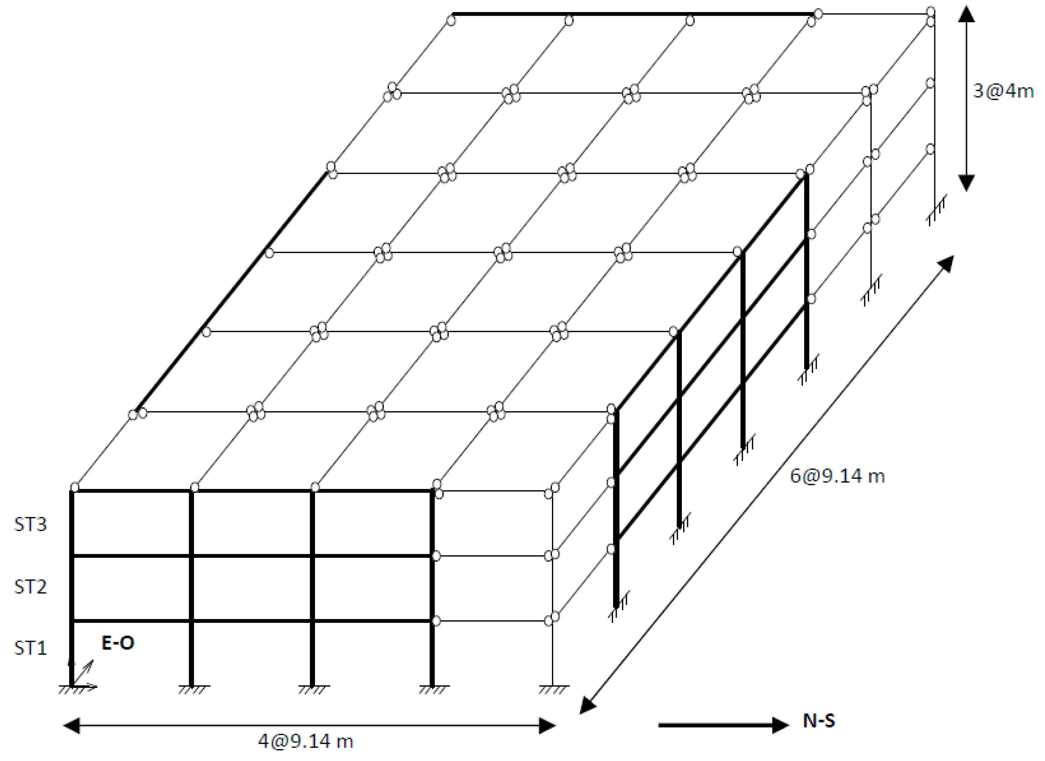
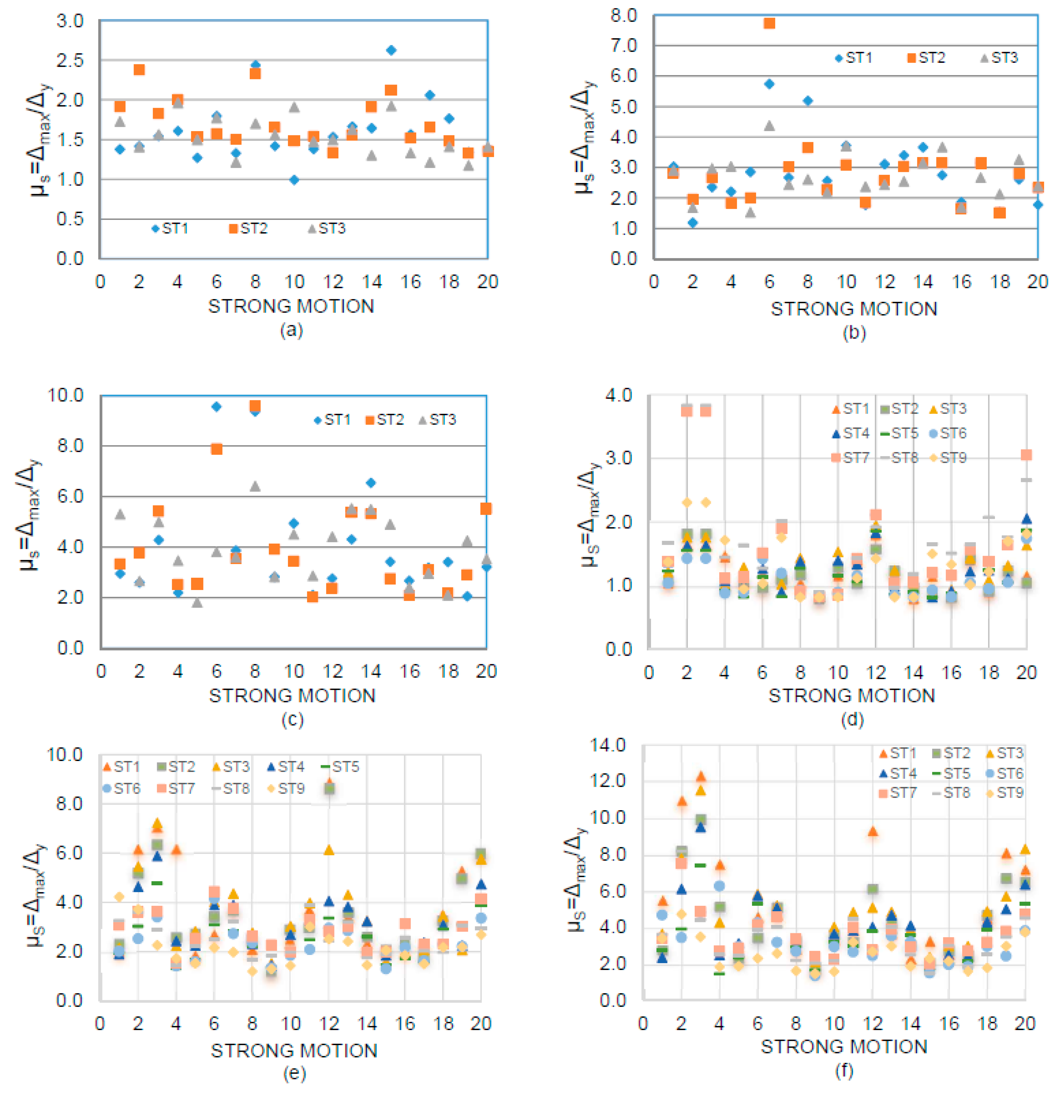
The local ductility parameter associated to bending, as defined by Equation (1), is calculated for all the structural members of both models for several intensities of the 20 strong motions as well as for the NS and EW directions. First, the models are subjected to the simultaneous action of the horizontal seismic component oriented in the EW direction, the vertical seismic component and the gravity loads. Then, the models are subjected to a similar set of loads, but the other horizontal component (NS direction) is considered instead. It is important to mention that even though, as stated earlier, the strong column–weak beam concept was considered in building design calculations, column hinging occurred in many cases.

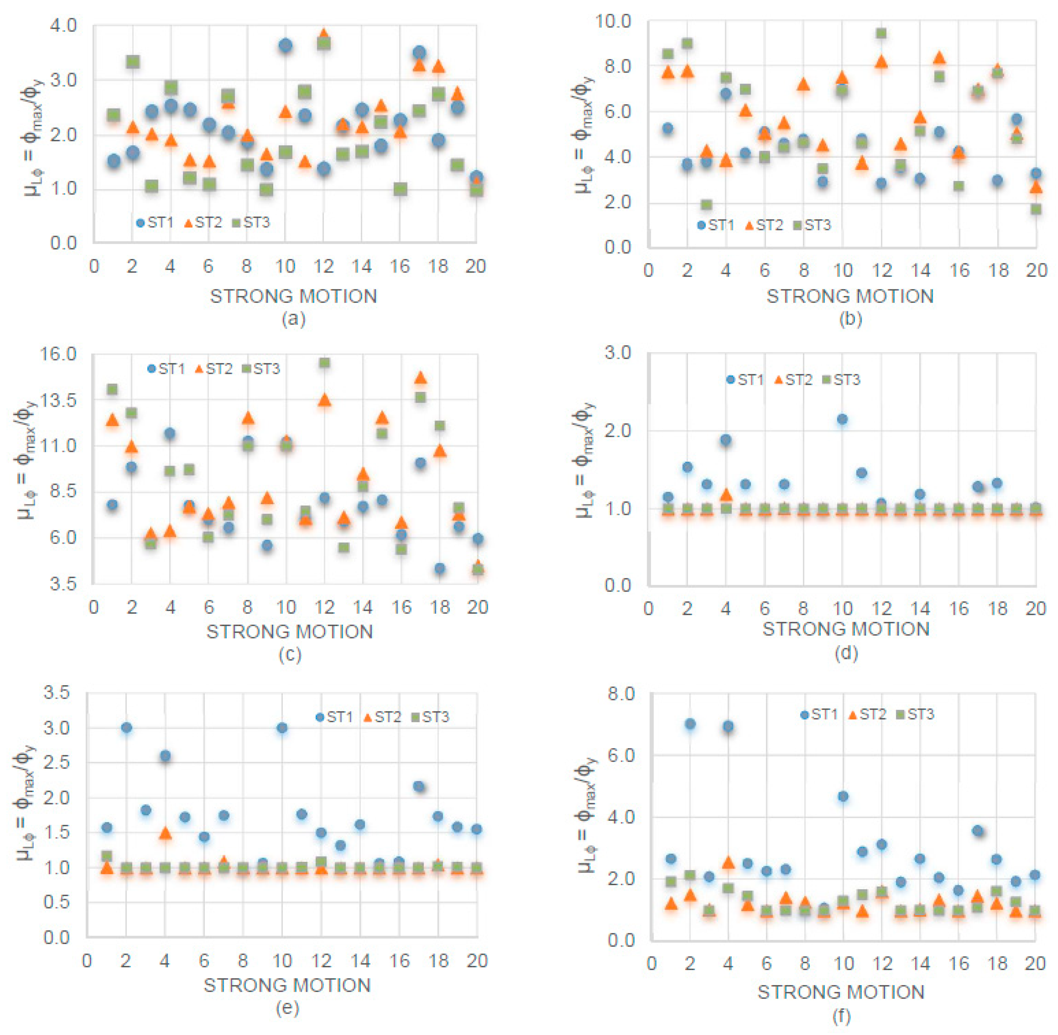
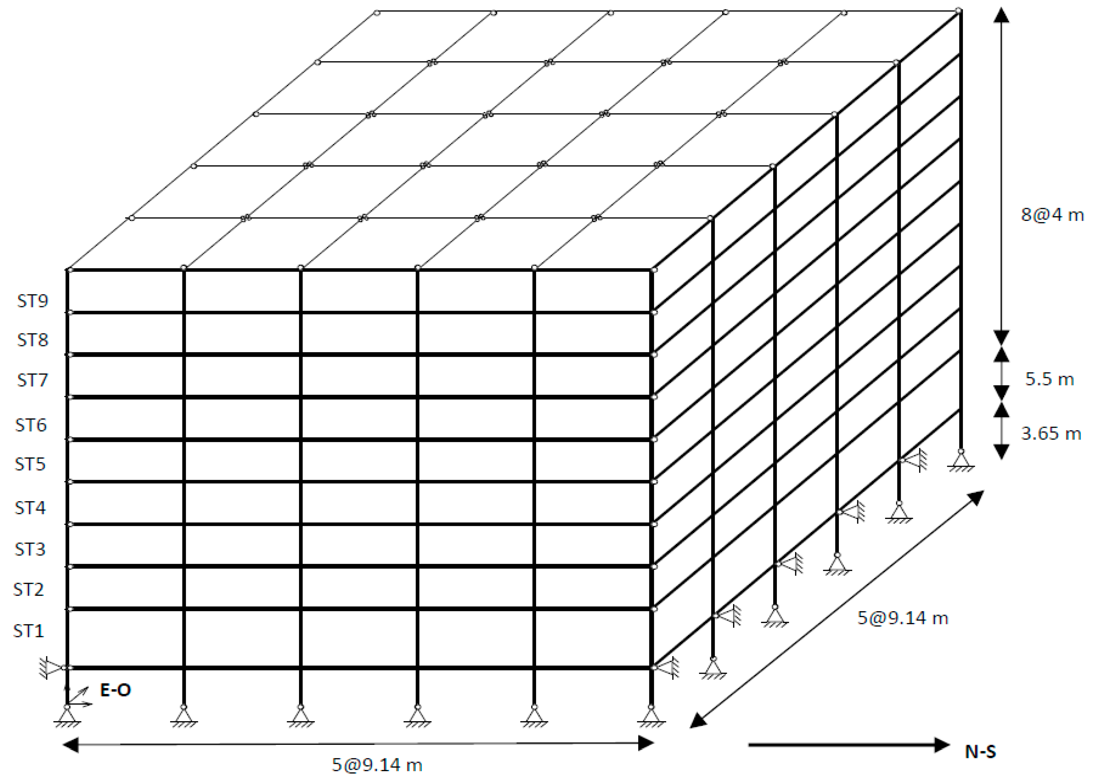
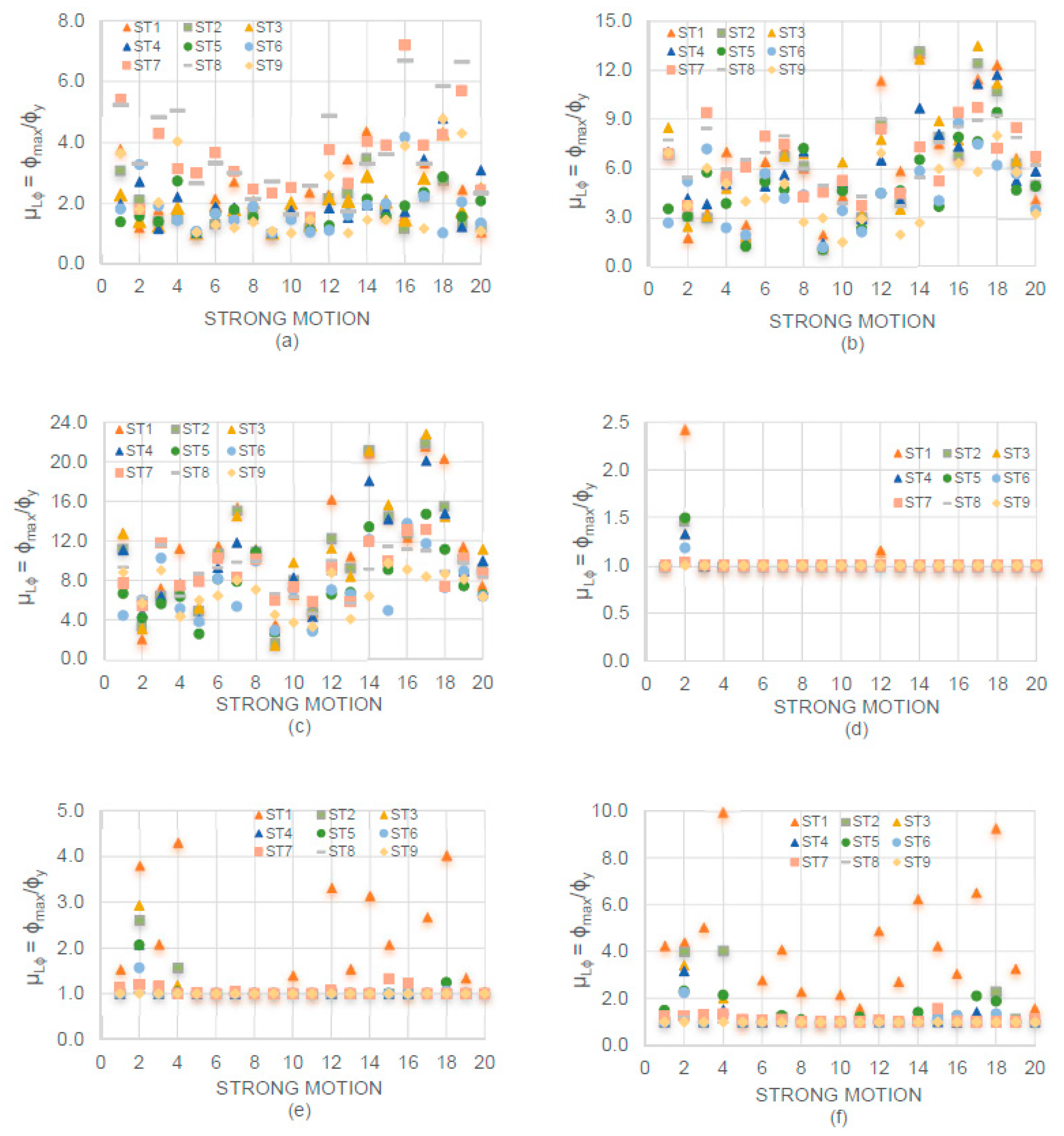
For a given story, the µ_Lϕ values are averaged, first over all the beams, and then over all the columns. The resulting averages for the beams of the 3-level building and the EW horizontal component, for seismic intensities S_a = 0.4 g, 0.8 g and 1.2 g, are presented in Figure 3a–c, respectively, while those associated to columns are given in Figure 3d–f, for the same strong motion intensities. The corresponding results for the 10-level building are presented in Figure 4, but in this case for seismic intensities of 0.2 g, 0.6 g and 0.8 g. In these figures, the symbol “ST” stands for the story level. It is worth to mention that moderate yielding occurs for seismic intensities of 0.4 g and 0.2 g for the 3- and 10-level structural models, respectively; the corresponding seismic intensities for significant deformations are 1.2 g and 0.8 g, for the 3- and 10-level models, respectively. In fact, even though it is not shown in the paper, the drifts for these significant levels of deformation were about 5% for some of the strong motions; the corresponding pattern of plastic hinges were very close to define a collapse mechanism. For this reason, the mentioned levels of maximum deformation are assumed to be associated the structural capacity of the models.

Results of the figures indicate that, for beams, the maximum values of µ_Lϕ (bending local ductility capacity) are about 15 and 20 for the 3- and 10-level buildings, respectively. There are some numerical and experimental [9,64,65] evidence that the bending local ductility capacity can reach values larger than 20; however, it is for monotonic loading and individual members. It is also observed that, for a given value of S_a, the magnitude of µ_Lϕ significantly varies from one seismic motion to another even though the seismic demands normalized according to S_a for each seismic motion was the same.

For example, for the case of beams of Story 3 of the 3-level building and S_a = 1.2 g, values as small as 4 and as larger as 15 are observed for the twentieth and twelfth strong motions, respectively. Such broad variation reflects the influence of the strong motion frequencies and the contribution of several vibration modes to the structural response. Results also indicate that the µ_Lϕ values increase as the seismic intensity increases and that the values are much larger for beams than for columns, as expected. Plots similar to those given in of Figure 3 and Figure 4 were also developed for the NS direction. In total 20 and 16 plots were developed for the 3- and 10-level buildings, respectively, but only the fundamental statistics in terms of the mean values (MV) and coefficients of variation (CV) are given for all cases; the results are presented in

Table 3. Statistics for µ_Lϕ, 3-level building.

Type of Member	Story	Dynamic Analysis																				PUSH
		NS Direction										EW Direction
		Sa/g Values										Sa/g Values
		0.4		0.6		0.8		1.0		1.2		0.4		0.6		0.8		1.0		1.2
		MV	CV	MV	CV	MV	CV	MV	CV	MV	CV	MV	CV	MV	CV	MV	CV	MV	CV	MV	CV
BEAMS	1	2.61	0.30	4.27	0.35	5.99	0.40	8.23	0.36	10.22	0.37	2.19	0.21	3.56	0.20	4.56	0.23	6.33	0.17	7.81	0.20	13.01
	2	2.48	0.28	4.60	0.33	7.17	0.26	9.57	0.25	11.86	0.26	2.26	0.22	4.15	0.25	5.87	0.26	7.69	0.26	9.32	0.27	16.64
	3	2.01	0.33	4.31	0.37	6.71	0.30	8.94	0.26	11.20	0.28	1.99	0.37	3.73	0.36	5.59	0.36	7.67	0.32	9.30	0.30	16.32
COLUMNS	1	1.06	0.09	1.32	0.28	1.95	0.44	2.65	0.47	3.70	0.51	1.01	0.02	1.25	0.19	1.72	0.24	2.22	0.32	2.87	0.39	1.00
	2	1.00	0.05	1.00	0.07	1.09	0.10	1.25	0.29	1.41	0.29	1.00	0.07	1.01	0.02	1.03	0.05	1.21	0.23	1.29	0.19	1.40
	3	1.00	0.04	1.00	0.06	1.06	0.05	1.12	0.15	1.23	0.23	1.00	0.03	1.00	0.04	1.02	0.02	1.13	0.14	1.26	0.24	8.71

and

Table 4. Statistics for µ_Lϕ, 10-level building.

Type of Member	Story	Dynamic Analysis																PUSH
		NS Direction								EW Direction
		Sa/g Values								Sa/g Values
		0.2		0.4		0.6		0.8		0.2		0.4		0.6		0.8
		MV	CV	MV	CV	MV	CV	MV	CV	MV	CV	MV	CV	MV	CV	MV	CV
BEAMS	2	1.93	0.34	5.60	0.40	9.91	0.41	14.69	0.35	1.60	0.33	4.65	0.39	8.10	0.39	11.89	0.37	1.60
	3	1.65	0.44	5.23	0.33	8.94	0.32	12.82	0.29	1.29	0.31	4.38	0.40	7.51	0.39	10.64	0.38	4.16
	4	1.83	0.38	5.47	0.28	8.61	0.28	12.61	0.23	1.41	0.26	4.58	0.41	7.58	0.40	10.80	0.36	8.02
	5	1.89	0.48	5.18	0.27	8.18	0.20	11.36	0.20	1.41	0.32	4.21	0.36	6.97	0.37	9.96	0.33	11.06
	6	1.56	0.48	4.11	0.32	6.46	0.23	8.68	0.20	1.20	0.24	3.44	0.33	5.49	0.35	7.71	0.36	15.62
	7	1.42	0.54	3.75	0.40	5.91	0.25	7.77	0.23	1.26	0.30	3.24	0.35	5.14	0.34	7.21	0.29	20.75
	8	2.61	0.41	4.96	0.29	6.58	0.21	8.36	0.22	2.53	0.30	4.70	0.25	6.33	0.22	7.97	0.23	23.15
	9	3.01	0.55	5.04	0.34	6.48	0.26	7.84	0.21	2.66	0.35	4.82	0.22	6.22	0.19	7.88	0.20	22.38
	10	2.11	0.62	3.74	0.45	5.09	0.36	6.32	0.24	1.49	0.53	3.27	0.35	4.85	0.26	6.34	0.25	21.15
COLUMNS	2	1.00	0.07	1.71	0.26	3.61	0.66	6.51	0.63	1.00	0.04	1.41	0.49	2.87	0.47	4.80	0.48	1.00
	3	1.00	0.05	1.00	0.04	1.57	0.72	2.54	0.74	1.00	0.04	1.00	0.08	1.90	0.43	1.54	0.46	1.00
	4	1.00	0.06	1.00	0.04	1.00	0.05	1.87	0.67	1.00	0.09	1.00	0.07	1.00	0.05	1.37	0.41	1.00
	5	1.00	0.03	1.00	0.03	1.00	0.04	1.64	0.49	1.00	0.03	1.00	0.04	1.00	0.06	1.31	0.29	1.00
	6	1.00	0.01	1.00	0.02	1.00	0.03	1.46	0.47	1.00	0.05	1.00	0.04	1.00	0.04	1.26	0.32	1.00
	7	1.00	0.01	1.00	0.02	1.00	0.02	1.00	0.04	1.00	0.02	1.00	0.05	1.00	0.03	1.00	0.04	1.00
	8	1.00	0.03	1.00	0.01	1.00	0.01	1.00	0.03	1.00	0.03	1.00	0.03	1.00	0.05	1.00	0.06	1.60
	9	1.00	0.02	1.00	0.01	1.00	0.01	1.00	0.02	1.00	0.01	1.00	0.03	1.00	0.02	1.00	0.04	3.60
	10	1.00	0.02	1.00	0.00	1.00	0.01	1.00	0.01	1.00	0.00	1.00	0.02	1.00	0.01	1.00	0.01	8.73

.

It can be observed from the tables that for the beams of the 3-level building, the maximum bending ductility demands occur, in general, for the second story. For the case of columns, as observed from individual graphs, the mean values are much smaller than those of beams; in fact for the two lowest intensities (S_a = 0.4 g and 0.6 g) they are essentially equal to unity for the two upper stories implying no yielding. Unlike what observed for beams, the mean values of µ_Lϕ for columns tend to decrease with the story number. For both, beams and columns, the mean values tend to increase with the seismic intensity and are larger for the NS that for the EW direction; the uncertainty in the estimation is moderate in most of the cases.

The statistics for the 10-level building (Table 4) resemble those of the 3-level building in the sense that the mean values of µ_Lϕ are much larger for beams than for columns and that the uncertainty in the estimation is, in general, moderate. However, unlike the 3-level building, the mean values tend to decrease with the story number for beams, and as for the 3-story building the µ_Lϕ mean values tend to decrease with the story number for columns; no yielding occurs in columns in most of the cases for low intensities of the strong motions (S_a = 0.2 g and 0.4 g). The only additional observation that can be made is that, for the larger strong motion intensities, the maximum mean values of the bending local ductility demands are observed to be larger for the 10-level building.

Local ductility values associated to axial elongations (µ_Lδ) were also calculated. It is worth to mention that since axial deformations of beams are negligible in comparison with those of bending, µ_Lδ is not calculated for beams. In other words, plasticization of beams (formation of plastic hinges) is essentially produced by bending. In addition, it was observed that, due to their location, the axial loads at interior columns are smaller than that of exterior columns in such a way that plasticization of interior columns are essentially due to the action of bending moments too. Thus, that the µ_Lδ parameter is calculated only for exterior columns

Similar to the case of µ_Lϕ, for a given story and building, the µ_Lδ values are averaged (but in this case only over the two exterior columns) and graphs for individual members are developed; only the fundamental statistics for the 3-level building are presented (

Table 5. Statistics for (µ_Lδ) for columns of the 3-level building.

Story	NS Direction										EW Direction
	Sa/g Values										Sa/g Values
	0.4		0.6		0.8		1.0		1.2		0.4		0.6		0.8		1.0		1.2
	MV	CV	MV	CV	MV	CV	MV	CV	MV	CV	MV	CV	MV	CV	MV	CV	MV	CV	MV	CV
1	1.00	0.00	1.00	0.00	1.00	0.00	1.00	0.00	1.00	0.00	1.00	0.00	1.00	0.00	1.00	0.00	1.00	0.00	1.00	0.00
2	1.00	0.00	1.00	0.00	1.00	0.00	1.03	0.13	1.26	0.62	1.00	0.00	1.00	0.00	1.07	0.29	1.11	0.44	1.23	0.57
3	1.39	0.46	2.54	0.85	2.34	0.79	2.20	0.61	2.58	0.59	1.15	0.22	1.96	0.76	3.94	0.73	4.48	0.73	3.57	0.54

), however. The main observations that can be made are that the mean values of µ_Lδ are comparable to those of µ_Lϕ for columns but much smaller than those of µ_Lϕ for beams. However, unlike the case of µ_Lϕ for beams or columns, the maximum values occur for the upper story.

The previous discussion clearly indicates that the ductility demands associated to column axial deformations of steel framed structures are much smaller than those associated to bending of beams; for example, for the 3-level building and the deformation state close to collapse (S_a = 1.2 g), the average ductility demand associated to bending of beams ranges from 7.8 to 11.86, while that associated to axial elongation on columns ranges from 1.00 to 3.57. Thus, even though tensional ductility demands are considered as an important issue in some research reports [9] and steel structural members may have a high ductility capacity in tension, these types of ductility demands are less relevant for the type of the structural system under consideration.

7. Objective 2: Story and Global Ductility, Dynamic Analysis

7.1. Story Ductility

The µ_S values for the NS direction of the 3-level building, calculated according to Equation (3), are shown in Figure 5a–c, for seismic intensities of 0.4 g, 0.8 g, and 1.2 g, respectively; while those of the 10-level building for the same direction are given in Figure 5d–f, for seismic intensities of 0.2 g, 0.6 g, and 0.8 g, respectively. These results resemble those of µ_Lϕ in the sense that they do not show any trend with the strong motions; the additional observation that can be made is that bending local ductility values are, in general, larger than those of story ductility. The fundamental statistics, for all the seismic intensities and structural directions under consideration, are presented in

Table 6. Statistics for µ_S, 3-level building.

Story	Dynamic analysis																				PUSH
	NS direction										EW direction
	Sa/g values										Sa/g values
	0.4		0.6		0.8		1.0		1.2		0.4		0.6		0.8		1.0		1.2
	MV	CV	MV	CV	MV	CV	MV	CV	MV	CV	MV	CV	MV	CV	MV	CV	MV	CV	MV	CV
1	1.61	0.24	1.99	0.34	2.81	0.40	3.44	0.51	3.95	0.55	1.48	0.20	1.90	0.31	2.80	0.37	2.89	0.34	4.28	0.69	8.63
2	1.70	0.18	2.20	0.29	2.86	0.46	3.31	0.42	3.99	0.50	1.65	0.17	2.15	0.24	2.58	0.31	3.09	0.32	3.54	0.45	7.66
3	1.53	0.16	1.93	0.20	2.69	0.27	2.99	0.23	3.90	0.33	1.52	0.24	2.10	0.24	2.72	0.29	3.19	0.37	3.84	0.42	6.87

and

Table 7. Statistics for µ_S, 10-level building.

Story	Dynamic Analysis																PUSHEr
	NS Direction								EW Direction
	Sa/g Values								Sa/g Values
	0.2		0.4		0.6		0.8		0.2		0.4		0.6		0.8
	MV	CV	MV	CV	MV	CV	MV	CV	MV	CV	MV	CV	MV	CV	MV	CV
2	1.21	0.23	2.23	0.51	3.77	0.56	5.19	0.59	1.04	0.16	1.73	0.32	2.66	0.42	3.95	0.51	5.90
3	1.18	0.25	2.11	0.37	3.57	0.51	4.40	0.50	1.05	0.20	1.90	0.38	2.57	0.44	3.63	0.45	6.59
4	1.29	0.24	2.35	0.45	3.52	0.46	4.79	0.48	1.24	0.27	2.11	0.36	2.91	0.41	3.88	0.43	7.62
5	1.26	0.27	2.13	0.34	3.10	0.38	4.12	0.45	1.13	0.24	1.96	0.33	2.74	0.36	3.41	0.39	6.88
6	1.15	0.29	1.88	0.38	2.56	0.36	3.38	0.43	1.04	0.16	1.70	0.31	2.54	0.35	2.93	0.35	5.07
7	1.12	0.31	1.77	0.40	2.32	0.33	3.14	0.38	1.08	0.19	1.66	0.31	2.06	0.34	2.77	0.40	3.97
8	1.64	0.54	2.23	0.47	2.88	0.27	3.55	0.35	1.44	0.24	2.21	0.24	2.81	0.28	3.14	0.35	3.78
9	1.76	0.48	2.32	0.30	2.54	0.28	3.31	0.45	1.57	0.26	2.32	0.31	2.71	0.22	3.40	0.34	2.43
10	1.33	0.36	1.74	0.34	2.18	0.36	2.49	0.35	1.17	0.26	1.60	0.28	2.17	0.29	2.63	0.33	5.90

, for the 3- and 10-level buildings, respectively. It can be observed that, as for the case of µ_Lϕ, the mean values of µ_S do not present any tendency with the story number for the case of the 3-level building; for the 10-level building, unlike the case of µ_Lϕ the values do not tend to decrease with high.

By comparing the results of Table 6 and Table 7 with those of Table 4 and Table 5, it is concluded that, as observed from individual plots, µ_S is much smaller than µ_Lϕ of beams; the values for the maximum seismic intensity range from 3.84 to 4.28 and from 2.49 to 5.19 for the 3- and 10-level models, respectively. As for µ_Lϕ for beams, the mean values and the uncertainty in the estimation tend to increase with the seismic intensity, however the uncertainty in the estimation is larger for µ_S.

7.2. Global Ductility

The global ductility values, calculated according to the two definitions under consideration (µ_GS and µ_Gt), are now discussed. The results are given in

Table 8. Global ductility (µ_GS y µ_Gt), 3-level building.

DEFIN	Dynamic Analysis										PUSH
	NS Direction					EW Direction
	Sa/g Values					Sa/g Values
	0.4	0.6	0.8	1.0	1.2	0.4	0.6	0.8	1.0	1.2
µGS	1.61	2.04	2.79	3.25	3.95	1.55	2.05	2.70	3.05	3.89	7.72
µGt	2.45	3.21	4.31	5.84	6.91	2.57	3.30	4.88	4.88	6.50	8.37

and

Table 9. Global ductility (µ_GS y µ_Gt), 10-level building.

DEFIN	Dynamic Analysis								PUSH
	NS Direction				EW Direction
	Sa/g Values				Sa/g Values
	0.2	0.4	0.6	0.8	0.2	0.4	0.6	0.8
µGS	1.27	2.08	2.94	3.82	1.18	1.91	2.57	3.31	5.08
µGt	8.40	11.70	22.40	36.34	4.89	13.52	25.51	38.78	7.98

, for the 3- and 10-level buildings, respectively. It can be observed that the values of µ_GS tend to increase (as expected) with the strong motion intensity and that they are larger for the 3- than for the 10-level building; for the ductility demands (ductility capacity) associated to the maximum deformations µ_GS takes values of 3.95 and 3.89, for the NS and EW direction, respectively, for the 3-level building, while the corresponding values are 3.82 and 3.31 for the 10-level building. By comparing the results of Table 8 and Table 9 with those of µ_Lϕ for beams (Table 3 and Table 4) it is noted that, as for the case µ_S, the values are significantly smaller for µ_GS. Most of the observations made µ_GS also apply to µ_Gt; however, unreasonable large values are observed for the latter, values of 36.34 and 38.78 were obtained for the 10-level buildings. The reason for this is not that very large drifts were obtained, but the top displacements when first yielding occurs in the buildings were very small indicating an important participation of the higher modes in the response. The implication of this is that the ductility definition based on the building top displacement, even though used in the profession, is not appropriate for the case of dynamic analysis, particularly for high buildings where significant structural contributions of the higher modes are expected.

8. Objective 3: Ductility According to Pushover Analysis

It is accepted that nonlinear time history analysis is the most accurate and reliable analysis procedure as long as realistic modeling of the structure and the cyclic load deformation characteristics of its structural elements are provided. The latter characteristic cannot be considered in pushover analysis implying that the effect of the dissipation of energy on the seismic response is neglected. Despite this, nonlinear static procedures are broadly used to estimate seismic responses in terms of different parameter for low- and medium-rise buildings. In this section of the paper, the different types of ductility under consideration are calculated by using pushover analysis and compared to those of dynamic analysis. The pattern of loads is the classical one where a triangular distribution is used; gravity loads were also considered. In order to have a reasonable comparison, the maximum drifts considered in pushover analysis (about 5%) is quite similar to those observed in dynamic analysis for many strong motions for the case of maximum seismic intensity (S_a = 1.2 g and 0.8 g for the 3- and 10-level buildings).

Similar to the case of dynamic analysis, as the lateral loads are gradually increased, the structural deformations are gradually increased too. As soon the first plastic hinge is developed in a particular member, in any member of a story, or in any member of the structure, the corresponding deformations ϕ_y, Δ_y and D_y,t as indicated in Equations (1), (3), and (5), respectively, are recorded. Then, by considering the associated maximum deformations (ϕ_max, Δ_max and D_max,t) the values of local, story and global ductility are calculated.

The results for bending local ductility are shown in last column of Table 3 for the 3-level building. As for the case of dynamic results, the values are much larger for beams than for columns. It is observed that for beams, the values of µ_Lϕ of pushover analysis, which range from 13.01 to 16.64, can be much larger than the µ_Lϕ mean values of dynamic analysis (ranging from 7.81 to 11.86). There are several reasons for this: (a) as stated earlier, the maximum drift was approximately the same for both type of analyses, however, it was observed for many but not for all the strong motions in the case of dynamic analysis, for many of them the maximum drift were about 4% for the maximum seismic intensity, (b) for the case of pushover, the drifts were very close to 5% for all stories, but for dynamic analysis values of 3% and even smaller were observed for some stories, (c) the drift at which first yielding occurred for the stories were smaller for pushover than for of dynamic analysis. Results also indicate that for the case of columns, µ_Lϕ values may be larger or smaller than those of dynamic analysis; however, the values tend to increase and decrease with the story number for pushover and dynamic analysis, respectively, showing an opposite trend.

The µ_Lϕ pushover results for the 10-level building are shown in last column of Table 4. The major observations made before for the 3-level building apply to this building: (a) the pushover values are larger for beams than for columns (in both cases tend to increase with the story number), (b) for the case of beams, the maximum pushover values are larger than the maximum dynamic mean values, and (c) for beams and columns, the values tend to increase and decrease with the story number for pushover and dynamic analysis, respectively. The additional observation that can be made is that for the case of beams, the maximum pushover or dynamic values are larger for the 10- than for the 3-level buildings. The µ_S values for pushover analysis are given in last columns of Table 6 and Table 7 for the 3- and 10-level models, respectively. It can be observed that, as for bending ductility demands of beams, µ_S in general is larger for pushover than for dynamic analysis. It is also shown that the values are larger for the 3- than for the 10-level building and that for the 3-level building the values tend to slightly decrease with the story number which is not observed for the 10-level building.

The global ductility values, as for the case of dynamic analysis, are calculated in terms of interstory displacements (µ_GS) and of top displacements (µ_Gt). The results are shown in last columns of Table 8 and Table 9. As for µ_S, µ_GS is larger for pushover (7.72 and 5.08) than for dynamic analysis (3.95 and 3.32) for both models. µ_Gt is larger for pushover than for dynamic analysis for the 3-level building, but unlike the case of dynamic analysis reasonable large values are observed for the case of the 10-level building.

9. Objective 4: Relationship between Local and Global Ductility

In experimental studies the ductility capacity is usually obtained for individual members (local ductility), for this reason, as stated earlier, it is suggested [10] considering local ductility as the basis for design. Thus it results convenient relate local to global ductility. In this section the ratio of global to local ductility, denoted by the R_LG parameter is presented and discussed. The ratio is calculated only for bending local ductility (µ_Lϕ) and global ductility, according to the two definitions under consideration (µ_GS y µ_Gt), for dynamics and pushover analysis. The results are summarized in

Table 10. Statistics of the R_LG ratio.

Definition	Model	Dynamic Analysis				Pushover
		EO		NS
		MV	CV	MV	CV
µGS	3-LEVEL	0.41	0.45	0.34	0.27	0.50
	10-LEVEL	0.35	0.33	0.32	0.19	0.36
µGt	3-LEVEL	0.79	NA	0.59	NA	0.55
	10-LEVEL	2.87	NA	2.59	NA	0.56

NA = not applicable.

.

It is observed that the R_LG values associated to µ_Gt and dynamic analysis give unreasonable larger values particularly for the 10-story building; the reason for this is that, as mentioned in Section 7, the normalizing quantity D_y,t in Equation (5) may be very small. These values are larger than that of pushover analysis which in turn are larger than those of µ_GS and dynamic analysis. Considering that: (a) µ_Gt of dynamic analysis fails addressing the normalizing quantity (D_y,t in Equation (5)) giving unreasonable large values of µ_Gt, (b) pushover does not take into account dissipation of energy, (c) SCWB concept was followed in the building design, and (d) the local axial ductility is not important in framed steel building structures, the ratio of global to local ductility capacity, proposed in this study, is calculated as the ratio of µ_GS to µ_Lϕ of beams for dynamic analysis. Results from the table indicate that, for this definition, the mean values of R_LG and the uncertainty in the estimation are larger for the 3- than for the 10-level building and larger for the EW than for the NS direction. Based on the values obtained in this study (0.41, 0.34, 0.35 and 0.32) a value of 1/3 is proposed for the R_LG ratio. Thus, if local ductility capacity is stated as the basis for the design, say 15 or 12, the global ductility capacity can be estimated as 5 or 4.

10. Conclusions

A numerical investigation regarding ductility evaluation of steel buildings with moment resisting steel frames is conducted in this paper. Some steel model buildings and some strong motions used in the SAC steel project are used in the study. Bending local (µ_Lϕ) and tension local (µ_Lδ) ductilities, story ductility (µ_S) as well as global ductility are studied; the most appropriate definition of global ductility is identified. Global ductility is calculated as the mean values of story ductilities (µ_GS) and as the ratio of the maximum inelastic top displacement to the top displacement when yielding occurs for the first time (µ_Gt). The ductility values calculated according to dynamic analysis are compared to those of pushover analyses. Results of the study indicate that the ductility values significantly may vary with the strong motion, the ductility definition, the structural element, the story number, the type of analysis, and the structural model. The main conclusions are:

(1)

For beams and columns and the maximum seismic intensity, the mean values of µ_Lϕ tend to decrease with the story number; however, as expected, the beam values are much larger than those of columns (10.22 and 14.69 against 4.8 and 6.51). The µ_Lδ values are only significant for exterior columns and much smaller than that of µ_Lϕ for beams. Even though tensional ductility demands are considered as an important issue in some research reports, and steel structural members may have a high ductility capacity in tension, these type of ductility is less relevant for the structural system under consideration.

(2)

The µ_S values for the maximum seismic intensity range from 3.84 to 4.28 and from 2.49 to 5.19 for the low- and medium-rise models, respectively. The values of µ_GS for dynamic analysis associated to the maximum seismic intensity (ductility capacity) are larger for the low- than for the medium-rise building (3.95 and 3.89 against 3.82 and 3.31). Unreasonable large values are obtained for µ_Gt, values of 36.34 and 38.78 were obtained for the 10-level buildings. The implication of this is that the ductility definition based on the building top displacement, even though used in the profession, is not appropriate for the case of dynamic analysis, particularly for high buildings where significant structural contributions of the higher modes are expected.

(3)

As for the case of dynamic results, the ductility values obtained from pushover analysis are much larger for beams than for columns. For beams, the values of µ_Lϕ, µ_S and µ_GS obtained from pushover can be much larger than the corresponding values obtained from dynamic analysis.

(4)

The ratio (R_LG) of global to local ductility (µ_Lϕ) is also calculated. Considering that: (a) µ_Gt for dynamic analysis results in unreasonable large values, (b) pushover analysis does not take into account for dissipation of energy, (c) SCWB concept was followed in the building design, and (d) the local axial ductility is not important in framed steel building structures, the R_LG ratio of dynamic analysis associated to bending local ductility is assumed to be the most appropriated definition. A value of 1/3 is proposed for this ratio. Thus, if local ductility capacity is stated as the basis for the design, say 15 or 12, the global ductility capacity can be estimated as 5 or 4.

References

1. International Code Council. International Building Code; International Code Council: Falls Church, VA, USA, 2009. [Google Scholar]
2. National Research Council of Canada. National Building Code of Canada (NBCC); National Council of Canada: Ottawa, ON, Canada, 2005.
3. Mexico City Building Code (MCBC). Complementary Technical Norms for Earthquake Resistant Design; MCBC: Mexico City, Mexico, 2004. [Google Scholar]
4. Committee Euripean of Normalisation. Design of Structures for Earthquake Resistance; CEN: Brussels, Belgium, 2004. [Google Scholar]
5. SAC. Steel Moment Frame Connections; Advisory No. 3 D-146; Structural Engineers Associated of California, Applied Technology Council and California University for Research in Earthquake Engineering: Sacramento, CA, USA, 1995. [Google Scholar]
6. Reyes-Salazar, A. Ductility and Ductility Reduction Factor for MDOF systems. Struct. Eng. Mech. Int. J. 2002, 13, 369–385. [Google Scholar] [CrossRef]
7. Uang, C.M. Establishing R (or Rw) and Cd Factors for Building Seismic Provisions. J. Struct. Eng. ASCE 1991, 117, 19–28. [Google Scholar] [CrossRef]
8. Uang, C.M. Structural Overstrength and Limit State Philosophy in Seismic Design Provisions; Department of Civil Engineering, Northeastern University: Boston, MA, USA, 1991. [Google Scholar]
9. Newmark, N.M.; Hall, W.J. Earthquake Spectra and Design Monograph Series; Earthquake Engineering Research Institute: Berkeley, CA, USA, 1982. [Google Scholar]
10. Osteraas, J.D.; Krawinkler, H. Strength and Ductility Considerations in Seismic Design; Blume Earthquake Engineering Center, Stanford University: Stanford, CA, USA, 1990. [Google Scholar]
11. ATC (Applied Technology Council). Tentative Provisions for the Development of Seismic Regulation Buildings; Report No. ATC-3-06; ATC: Redwood City, CA, USA, 1978. [Google Scholar]
12. Hadjian, A.H. An Evaluation of the Ductility Reduction Factor Q in the 1976 Regulations for the Federal District of Mexico. Earthq. Eng. Struct. Dyn. 1989, 18, 217–231. [Google Scholar] [CrossRef]
13. Miranda, E.; Bertero, V. Evaluation of Strength Reduction Factors for Earthquake-Resistant Design. Earthq. Spectra 1994, 10, 357–379. [Google Scholar] [CrossRef]
14. Tiwari, A.K.; Gupta, V.K. Scaling of ductility and damage-based strength reduction factors for horizontal motions. Earthq. Eng. Struct. Dyn. 2000, 29, 969–987. [Google Scholar] [CrossRef]
15. Arroyo-Espinoza, D.; Teran-Gilmore, A. Strength reduction factors for ductile structures with passive energy dissipating devices. J. Earthq. Eng. 2003, 7, 297–325. [Google Scholar] [CrossRef]
16. Levy, R.; Rutenberg, A.; Qadi, K.H. Equivalent linearization applied to earthquake excitations and the R-µ-T0 relationships. Eng. Struct. 2006, 28, 216–228. [Google Scholar] [CrossRef]
17. Karmakar, D.; Gupta, V.K. A parametric study of strength reduction factors for elasto-plastic oscillators. Sādhanā 2006, 31, 343–357. [Google Scholar] [CrossRef] [Green Version]
18. Rupakhety, R.; Sigbjörnsson, R. Ground-motion prediction equations (GMPEs) for inelastic response and structural behavior factors. Bull. Earthq. Eng. 2009, 7, 637–659. [Google Scholar] [CrossRef]
19. Fanaie, N.; Dizaj, E.A. Response modification factor of the frames braced with reduced yielding segment BRB. Struct. Eng. Mech. 2014, 50, 1–17. [Google Scholar] [CrossRef]
20. Zahrai, S.M.; Jalali, M. Experimental and analytical investigations on seismic behavior of ductile steel knee braced frames. Steel Compos. Struct. 2014, 16, 1–21. [Google Scholar] [CrossRef]
21. Zhai, C.H.; Wen, W.P.; Li, S.; Xie, L.L. The ductility-based strength reduction factor for the mainshock–aftershock sequence-type ground motions. Bull. Earthq. Eng. 2015, 13, 2893–2914. [Google Scholar] [CrossRef]
22. Ghods, S.; Kheyroddin, A.; Nazeryan, M.; Mirtaheri, S.M.; Gholhaki, M. Nonlinear behavior of connections in RCS frames with bracing and steel plate shear wall. Steel Compos. Struct. 2016, 22, 915–935. [Google Scholar] [CrossRef]
23. Nassar, A.; Krawinkler, H. Seismic Demands of SDOF and MDOF Systems; John, A., Ed.; Blume Earthquake Engineering Center, Standford University: Stanford, CA, USA, 1991. [Google Scholar]
24. Santa-Ana, P.; Miranda, E. Strength Reduction Factors of Multi-Degree-of-Freedom Systems. In Proceedings of the 12th World Conference on Earthquake Engineering, Auckland, New Zealand, 30 January–4 February 2000. [Google Scholar]
25. Moghaddam, H.; Mohammadi, R.K. Ductility reduction factor of MDOF shear-building structures. J. Earthq. Eng. 2001, 5, 425–440. [Google Scholar] [CrossRef]
26. Elnashai, A.S.; Mwafy, A.M. Overstrength and force reduction factors of multistorey reinforced-concrete buildings. Struct. Des. Tall Build. 2002, 11, 329–351. [Google Scholar] [CrossRef]
27. Medina, R.; Krawinkler, H. Evaluation of drift demands for the seismic performance assessment of frames. J. Struct. Eng. ASCE 2005, 131, 1003–1013. [Google Scholar] [CrossRef]
28. Medina, R.; Krawinkler, H. Strength demand issues relevant for the seismic design of moment-resisting frames. Earthq. Spectra 2005, 21, 415–439. [Google Scholar] [CrossRef]
29. De Stefano, M.; Marino, E.M.; Rossi, P.P. Effect of Overstrength on the Seismic Behaviour of Multi-Storey Regularly Asymmetric Buildings. Bull. Earthq. Eng. 2006, 4, 23–42. [Google Scholar] [CrossRef]
30. Cai, J.; Zhou, J.; Fang, X. Seismic Ductility Reduction Factors for Multi-Degree-of-Freedom Systems. Adv. Struct. Eng. 2006, 9, 591–601. [Google Scholar] [CrossRef]
31. Chopra, A.K. Dynamics of Structures; Prentice Hall: Upper Saddle River, NJ, USA, 2007. [Google Scholar]
32. Mollaioli, F.; Bruno, S. Influence of side effects on inelastic displacement ratios for SDOF and MDOF systems. Comput. Math. Appl. 2008, 55, 184–207. [Google Scholar] [CrossRef]
33. Vielma, J.C.; Barbat, A.H.; Oller, S. Seismic safety of low ductility structures used in Spain. Bull. Earthq. Eng. 2010, 8, 135–155. [Google Scholar] [CrossRef]
34. Ceylan, M.; Arslan, M.H.; Ceylan, R.; Kaltakci, M.Y.; Ozbay, Y. A new application area of ANN and ANFIS: Determination of earthquake load reduction factor of prefabricated industrial buildings. Civ. Eng. Environ. Syst. 2010, 27, 53–69. [Google Scholar] [CrossRef]
35. Ganjavi, B.; Hao, H. Effect of structural characteristics distribution of strength demand and ductility reduction factor of MDOF systems considering soil-structure interaction. Earthq. Eng. Eng. Vib. 2012, 11, 205–220. [Google Scholar] [CrossRef]
36. Kumar, M.; Stafford, P.J.; Elghazouli, A.Y. Seismic shear demands in multi-storey steel frames designed according to Eurocode 8. Eng. Struct. 2013, 52, 69–87. [Google Scholar] [CrossRef]
37. Kumar, M.; Stafford, P.J.; Elghazouli, A.Y. Influence of ground motions characteristics on drift demands in steel moment frames designed according to Eurocode 8. Eng. Struct. 2013, 52, 502–517. [Google Scholar] [CrossRef]
38. Serror, M.H.; Diab, R.A.; Mourad, S.A. Seismic force reduction factor for steel moment resisting frames with supplemental viscous dampers. Earthq. Struct. 2014, 7, 1171–1186. [Google Scholar] [CrossRef]
39. Reyes-Salazar, A.; Bojórquez, E.; Velazquez-Dimas, J.I.; López-Barraza, A.; Rivera-Salas, J.L. Ductility and ductility reduction factors for steel buildings considering different structural representations. Bull. Earthq. Eng. 2015, 13, 1749–1771. [Google Scholar] [CrossRef]
40. Valenzuela-Beltrán, F.; Ruiz, S.E.; Reyes-Salazar, A.; Gaxiola-Camacho, J.R. On the Seismic Design of Structures with Tilting Located within a Seismic Region. Appl. Sci. 2017, 7, 1146. [Google Scholar] [CrossRef]
41. Fanaie, N.; Shamlou, S.O. Response modification factor of mixed structures. Steel Compos. Struct. 2015, 19, 1449–1466. [Google Scholar] [CrossRef]
42. Vuran, E.; Aydınoğlu, M.N. Capacity and ductility demand estimation procedures for preliminary design of coupled core wall systems of tall building. Bull. Earthq. Eng. 2016, 14, 721–745. [Google Scholar] [CrossRef]
43. Gómez-Martínez, F.; Alonso-Durán, A.; De Luca, F.; Verderame, G.M. Ductility of wide-beam RC frames as lateral resisting system. Bull. Earthq. Eng. 2016, 14, 1545–1569. [Google Scholar] [CrossRef] [Green Version]
44. Wang, B.; Dai, H.; Wu, T.; Bai, G.; Bai, Y. Experimental Investigation on Seismic Behavior of Steel Truss-RC Column Hybrid Structure with Steel Diagonal Braces. Appl. Sci. 2018, 8, 131. [Google Scholar] [CrossRef]
45. Liu, G.; Lian, J.; Liang, C.; Zhao, M. Structural response analysis in time and frequency domain considering both ductility and strain rate effects under uniform and multiple-support earthquake excitations. Earthq. Struct. 2016, 10, 989–1012. [Google Scholar] [CrossRef]
46. Hashemi, S.S.; Sadeghi, K.; Vaghefi, M.; Shayan, K. Evaluation of ductility and response modification factor in moment-resisting steel frames with CFT columns. Earthq. Struct. 2017, 12, 643–652. [Google Scholar] [CrossRef]
47. Kang, J.D.; Mori, Y. Evaluation of a Simplified Method to Estimate the Peak Inter-Story Drift Ratio of Steel Frames with Hysteretic Dampers. Appl. Sci. 2017, 7, 449. [Google Scholar] [CrossRef]
48. Reyes-Salazar, A.; Haldar, A. Dissipation of Energy in Steel Frames With PR Connections. Struct. Eng. Mech. Int. J. 2000, 9, 241–256. [Google Scholar] [CrossRef]
49. Reyes-Salazar, A.; Haldar, A. Energy Dissipation at PR Frames Under Seismic Loading. J. Struct. Eng. ASCE 2001, 127, 588–593. [Google Scholar] [CrossRef]
50. Reyes-Salazar, A.; Haldar, A. Seismic Response and Energy Dissipation in Partially Restrained and Fully Restrained Steel Frames: An Analytical Study. Steel Compos. Struct. Int. J. 2001, 1, 459–480. [Google Scholar] [CrossRef]
51. Roeder, C.W.; Scheiner, S.P.; Carpenter, J.E. Seismic Behavior of Moment-Resisting Steel Frames: Analytical Study. J. Struct. Eng. ASCE 1993, 119, 1866–1884. [Google Scholar] [CrossRef]
52. Leon, R.T.; Shin, K.J. Performance of Semi-Rigid Frames. In Proceedings of the Structure XIII Congress, Boston, MA, USA, 2–5 April 1995; pp. 1020–1035. [Google Scholar]
53. Nader, M.N.; Astaneh, A. Dynamic Behavior of Flexible, Semi-rigid and Rigid Frames. J. Constr. Steel Res. 1991, 18, 179–192. [Google Scholar] [CrossRef]
54. Osman, A.; Ghobarah, A.; Korol, R.M. Implications of Design Philosophies of Seismic Response of Steel Moments Frame. Earthq. Eng. Struct. Dyn. 1995, 24, 127–143. [Google Scholar] [CrossRef]
55. FEMA. State of the Art Report on Systems Performance of Steel Moment Frames Subject to Earthquake Ground Shaking, Prepared for the SAC joint Venture Partnership by Helmut Krawinkler; Report No. FEMA 355-C; FEMA: Washington, DC, USA, 2000.
56. Uniform Building Code (UBC). International Conference of Building Officials (ICBO), Whittier, CA, USA. 1997. [Google Scholar]
57. BOCA. 12th Edition Building Officials & Code Administration International; BOCA: Country Club Hills, IL, USA, 1993.
58. Carr, A. “RUAUMOKO” Inelastic Dynamic Analysis Program; University of Cantenbury, Department of Civil Engineering: Christchurch, New Zealand, 2011. [Google Scholar]
59. Chen, W.F.; Atsuta, T. Interaction Equations for Biaxially Loaded Sections; Fritz Laboratory Report (72-9); Leigh University: Bethlehem, PA, USA, 1972. [Google Scholar]
60. Aboosaber, M.; Hines, E.M. Modeling Reserve System Performance for Low-Ductility Braced Frames; Technical Report TUSSR-2011/1; Tufts University Structural Systems Research (TUSSR), Department of Civil and Environmental Engineering: Medford, MA, USA.
61. Amadio, C.; Chiara Bedon, CH.; Fasan, M.; Pecce, M.R. Refined numerical modelling for the structural assessment of steel-concrete composite beam-to-column joints under seismic loads. Eng. Struct. 2017, 138, 394–409. [Google Scholar] [CrossRef]
62. Christidis, A.A.; Dimitroudi, E.G.; Hatzigeorgiou, G.D.; Beskos, D.E. Maximum seismic displacements evaluation of Steel frames from their post-earthquake residual deformation. Bull. Earthq. Eng. 2013, 11, 2233–2248. [Google Scholar] [CrossRef]
63. Amadio, C.; Chiara Bedon, C.H.; Fasan, M. Numerical assessment of slab-interaction effects on the behaviour of steel-concrete composite joints. J. Construct. Steel Res. 2017, 139, 397–410. [Google Scholar] [CrossRef]
64. Liew, A.; Gardner, L.; Block, P. Moment-Curvature-Thrust Relationships for Beam-Columns. Structures 2017, 11, 146–154. [Google Scholar] [CrossRef] [Green Version]
65. Galambos, T.V. Structural Members and Frames; Prentice Hall: Englewood Cliffs, NJ, USA, 2016. [Google Scholar]
Figure 1. Isometric view of the 3-level building.
Applsci 09 00200 g001
Figure 2. Isometric view of the 9-level building.
Applsci 09 00200 g002
Figure 3. Bending local ductility (µ), EW direction, 3-level building; beams: (a) Sa = 0.4 g, (b) Sa = 0.8 g, (c) Sa = 1.2 g; columns: (d) Sa = 0.4 g, (e) Sa = 0.8 g, (f) Sa = 1.2 g.
Applsci 09 00200 g003
Figure 4. Bending local ductility (µ), EW direction, 10-level building; beams: (a) Sa = 0.2 g, (b) Sa = 0.6 g, (c) Sa = 0.8 g; columns: (d) Sa = 0.2 g, (e) Sa = 0.6 g, (f) Sa = 0.8 g.
Applsci 09 00200 g004
Figure 5. Story ductility (µS) values; NS direction; 3-level building: (a) Sa = 0.4 g, (b) Sa = 0.8 g, (c) Sa = 1.2 g; 10-level buildings: (d) Sa = 0.2 g, (e) Sa = 0.6 g, (f) Sa = 0.8 g.
Applsci 09 00200 g005