An Improved Skewness Balancing Filtering Algorithm Based on Thin Plate Spline Interpolation
by
 , , ,
, , ,
Penggen Cheng
1,2,3 ,
,
Zhenyang Hui
1,2,3,* ,
,
Yuanping Xia
1,2,3,
Yao Yevenyo Ziggah
4 ,
,
Youjian Hu
5 and
Jing Wu
1 1
Faculty of Geomatics, East China University of Technology, Nanchang 330013, China
2
Key Laboratory of Watershed Ecology and Geographical Environment Monitoring, NASG, Nanchang 330013, China
3
Key Laboratory for Digital Land and Resources of Jiangxi Province, East China University of Technology, Nanchang 330013, China
4
Faculty of Mineral Resources Technology, University of Mines and Technology, Tarkwa 999064, Ghana
5
Faculty of Information Engineering, China University of Geosciences, Wuhan 430074, China
*
Author to whom correspondence should be addressed.
Appl. Sci. 2019, 9(1), 203; https://0-doi-org.brum.beds.ac.uk/10.3390/app9010203
Submission received: 7 November 2018
/
Revised: 19 December 2018
/
Accepted: 3 January 2019
/
Published: 8 January 2019
(This article belongs to the Special Issue LiDAR and Time-of-flight Imaging)
Abstract
:Featured Application
DEM extraction from airborne LiDAR data.
Abstract
Most filtering algorithms suffer from complex parameter settings or threshold adjusting. To solve this problem, this paper proposes an improved skewness balancing filtering algorithm based on thin plate spline (TPS) interpolation. The proposed algorithm filters the nonground points in an iterative manner. A reference surface that reflects the fluctuation of the terrain is generated using the TPS interpolation method. Accordingly, the elevation difference from each point to the surface can be calculated. By applying the skewness balancing principle to these elevation differences, nonground points can be removed automatically. To verify the validity and robustness of the proposed method, the datasets provided by the International Society for Photogrammetry and Remote Sensing (ISPRS) were adopted. The experimental results show that this presented method can adapt to complex environments and achieve a higher filtering accuracy than the traditional skewness balancing algorithm. Moreover, in comparison with the other eight filtering methods tested by the ISPRS and four improved filtering methods proposed recently, the proposed method achieved an average total error of 5.39%, which is smaller than that of most of these other methods.
1. Introduction
In recent decades, the airborne light detection and ranging (LiDAR) technique has developed very quickly and become an one important means for acquiring remote sensing data [1,2]. The airborne LiDAR system is generally composed of a laser scanner, a global positioning system (GPS) and an inertial measurement unit (IMU) [3]. With these three components cooperating with each other, a large amount of LiDAR point clouds reflected from the ground and objects (cars, trees, buildings, etc.) can be obtained. Compared with traditional remote sensing methods, such as photogrammetric mapping, airborne LiDAR has the following advantages: (1) the external environment has little influence on the LiDAR technique; thus, an airborne LiDAR system can generally work in any environment and all-weather conditions; (2) LiDAR can describe the earth surface with a large number of points, which is beneficial for modeling; and (3) LiDAR pulses can penetrate the tree canopy, which makes this technique convenient for detecting topography in forest areas [4,5,6,7]. Owing to these advantages, airborne LiDAR has been applied to many applications, such as three-dimensional building model construction [8,9], power line inspection [10], change detection [11], and land cover classification [12].
To realize these applications, one key step is to obtain a digital terrain model (DTM). In other words, ground points should be separated from object points first. This process is called filtering. In the past two years, many researchers have been making efforts in this area, and diverse algorithms have been presented. These filtering algorithms can be classified into four categories: slope-based [13,14,15,16,17], morphology-based [18,19,20,21,22,23], triangular irregular network (TIN)-based [24,25,26,27] and segmentation-based [28,29,30] filtering algorithms.
The slope-based filtering algorithm was first proposed by Vosselman [14]. He assumed that terrain does not change greatly. That is, if the slope between two adjacent points is greater than a given threshold, there must be one point that belongs to an object. However, this assumption is false when encountering undulating terrain, such as cliffs or ridges. To solve this problem, Susaki [17] modified this method by adjusting thresholds based on local terrain. This improvement enables this method to achieve promising results in complicated environments.
Morphology-based filtering algorithms always adopt progressive strategies. The filtering thresholds are adaptively calculated as the filtering window changes gradually [23]. The main problem for this kind of approach is how to set an appropriate filtering window. A larger filtering window flattens terrain details, while a smaller filtering window cannot filter larger objects, such as building roofs. Hui et al. [7] improved the progressive morphology approach by combining it with multilevel Kriging interpolation. As a result, a smaller filtering error was achieved.
TIN-based approaches utilize a progressive manner to realize filtering. First, some located lowest points are selected as seed points and a rough TIN surface is built based on these ground seeds. Then, the iteration angle and distance of each point are calculated according to the TIN. The points are added to the TIN if their iteration angle and distance are less than the predefined thresholds. This process is iterated until no more points meet the requirements [24]. The built TIN is changed from coarser to finer while the filtering accuracy is progressively improved. Conversely, the initial built TIN has a great influence on the final filtering result. If the initial ground seeds are not selected correctly, the final filtering results will have a larger filtering error. To resolve this problem, Zhao et al. [26] applied morphological opening operations to obtain more potential ground seeds. Their experimental results show that this improvement enhances the robustness of this traditional method.
Segmentation-based filtering algorithms always rely on two main steps, namely, segmentation and filtering. In contrast to the abovementioned three kinds of methods, this kind of approach first applies some segmentation methods, such as region growing, for clustering the scatter points. Then, filtering is realized based on the segmentation results. Many researchers combine segmentation methods with traditional filtering algorithms and obtain good filtering performance. For example, Tovari and Pfeifer [28] modified the linear-prediction method proposed by Kraus and Pfeifer [31] using a region growing algorithm and improved the filtering accuracy at break lines. Since segmentation-based algorithms can use more semantic information, this kind of method generally performs much better than other kinds of methods. However, the performance of this kind of method relies heavily on the segmentation results. If the segmentation results are not accurate, a larger filtering error will be obtained.
The above-mentioned filtering methods are mainly proposed for airborne laser scanning (ALS) data. In addition to ALS, two other LiDAR techniques, namely, terrestrial laser scanning (TLS) and mobile laser scanning (MLS), are also developed vary fast. Thus, many researchers have been focusing on developing filtering algorithms for TLS or MLS data. Rodríguez-Caballero et al. [32] proposed an adaptive filtering for TLS point clouds using morphological filters and spectral information. In their method, the morphological filtering windows can be adapted to different types and sizes of plants. Thus, a more accurate representation of the soil surface can be obtained. In order to improve the accuracy, robustness and efficiency of the filtering method, Che and Olsen [33] proposed a fast ground filter for TLS data via scan line density analysis. By evaluating the local point density within a scan line, the ground candidates are first separated. The region growth algorithm is then used to get a better ground points clustering results. MLS owns a similar scan geometry to TLS. The main difference between MLS and TLS is that the scanner of MLS keeps continuously moving. Wu et al. [34] first organized the MLS data into vertical profiles and then candidate ground points were selected using an alpha shape algorithm. Li et al. [35] proposed a new filtering method to filtering ground surface points from MLS point clouds based on range constraint, slope constraint and angular position constraint.
From the aforementioned studies, it can be seen that although most filtering algorithms can obtain good filtering performance, almost all the approaches need to predefine parameter thresholds. For example, in the simple morphological filter (SMRF) algorithm proposed by Pingel et al. [22], after optimizing the parameters, the filtering total error decreased from 4.40% to 2.97%. In the progressive morphological filtering method proposed by Zhang et al. [23], five parameters need to be set. Generally, optimized parameters always lead to a better filtering result. Conversely, optimizing parameters is always time consuming. Moreover, determining an optimized parameter is generally for inexperienced researchers. For these reasons, some filtering algorithms with good performance in the literature are hard to use in practice.
To avoid complicated parameter settings, a statistical filtering algorithm called skewness balancing was developed by Bartels et al. [36]. In this unsupervised method, no parameters, such as a threshold or weighting factor, are required to be set. The algorithm can remove nonground points automatically. Moreover, this approach can achieve promising performance in flat areas. However, since this approach assumes that nonground points, such as building roofs, are always located above terrain, it is obvious that this method will cause a larger filtering error in fluctuating areas. To boost this method’s adaptability to complicated environments, this paper proposes an improved skewness balancing filtering algorithm based on thin plate spline (TPS) interpolation. The proposed algorithm filters the nonground points in an iterative manner. A reference surface that reflects the fluctuation of the terrain is generated using the TPS interpolation method. Accordingly, the elevation difference from each point to the surface can be calculated. By applying the skewness balancing principle to these elevation differences, nonground points can be removed automatically. The proposed algorithm was tested using the datasets provided by the International Society for Photogrammetry and Remote Sensing (ISPRS). The experimental results show that this presented method can adapt to complex environments and achieve a higher filtering accuracy than the traditional skewness balancing algorithm. Owing to the simple principle and high automation, the proposed method has the potential to contribute to the postprocessing of airborne LiDAR point clouds.
2. Materials and Methods
The proposed filtering algorithm based on progressive TPS interpolation is explained in the following subsections. Section 2.1 introduces the principle of the traditional skewness balancing algorithm, while the main problem of this traditional unsupervised method is illustrated by Figure 1 in Section 2.2. To resolve this problem, Section 2.3 presents the principle of the proposed method and explains the detailed implementation procedure, including point cloud denoising, selecting ground seeds, TPS interpolation, and filtering judgment.
2.1. Removing the Outliers Based on Morphological Operations
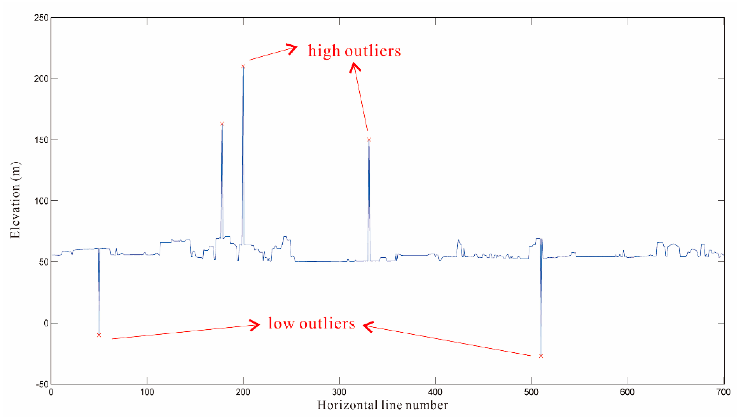
Due to the influence of external environments or the instrument itself, the obtained LiDAR point clouds always contain outliers. These outliers can be further classified as low and high outliers, as shown in Figure 1. High outliers are commonly generated by laser pulses reflected from aircraft or birds flying in the sky, while low outliers are always caused by multipath effects. Both of these kinds of outliers have a direct influence on the filtering results. Thus, both kinds of outliers should be removed before filtering.
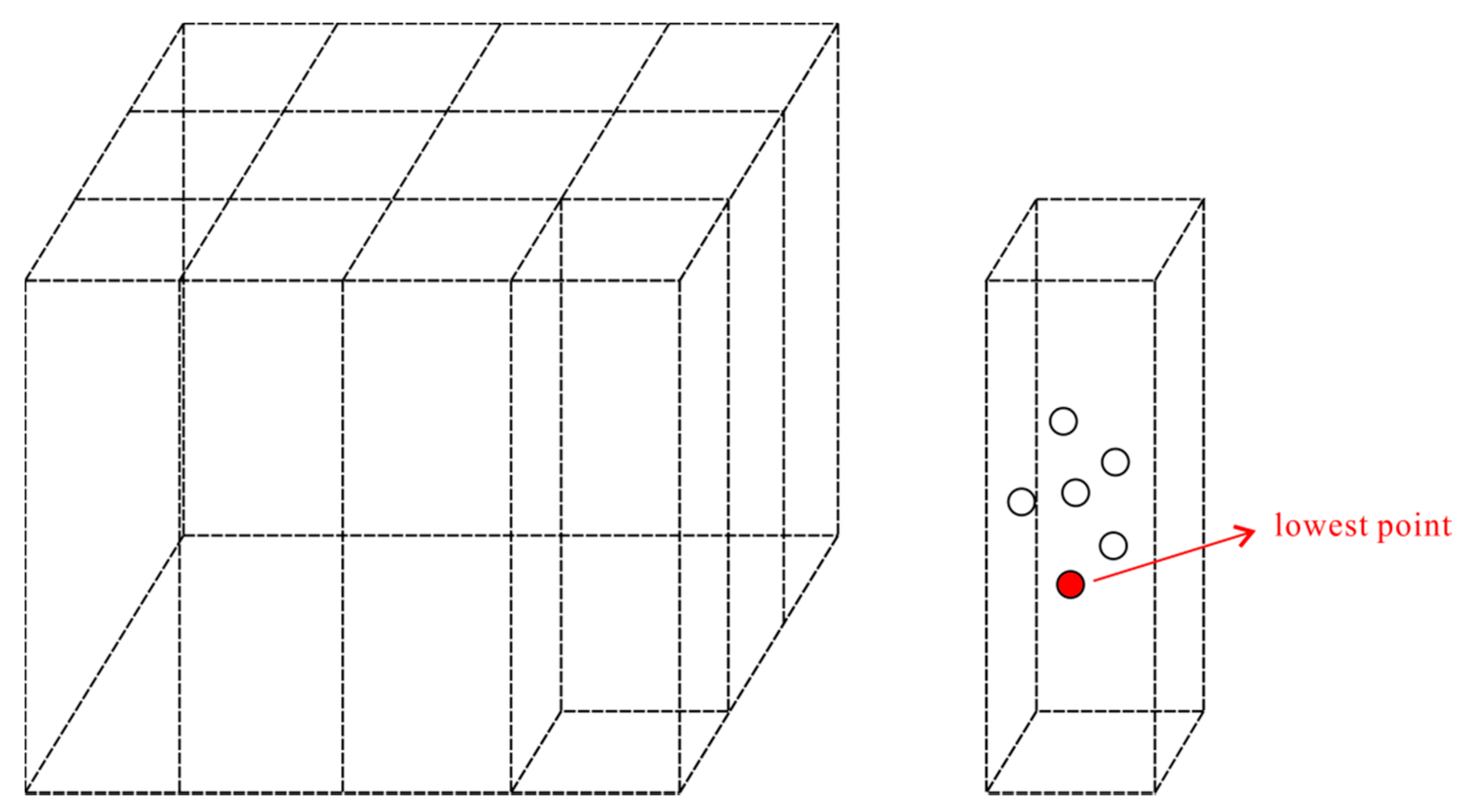
In this paper, the outliers are removed based on morphological operations. Since raw point clouds have no regular distribution, the LiDAR data should be organized first [37]. This paper organizes the 3-D LiDAR data as 2.5-D data using pseudo-grids, as shown in Figure 2. First, the cellsize of each grid should be defined according to the density of point clouds. In general, the cellsize is equal to , where is the density of point clouds. In so doing, we can try to make the grids with no points as few as possible. If there are more than one point falling into one grid, only the lowest elevation is kept as the characteristic value of the grid, as shown in Figure 2.
Generally, the outliers are isolated points and their elevations are far from the main body of the LiDAR points. Thus, this paper applies morphological dilation operation to the grids () generated in last step. If the characteristic value of a grid changes greatly before and after the morphological dilation, the grid is labeled as a noisy grid. This step can be denoted as Equation (1).
where is the characteristic value of the grid , is the characteristic value after morphological dilation, and is used to calculate the absolute value.
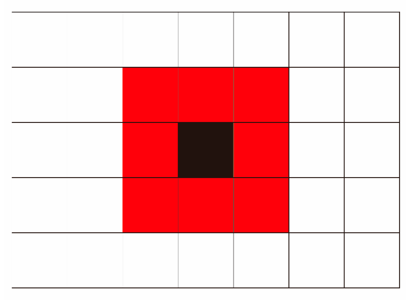
Morphological dilation is used to select the largest characteristic value in the structure element [23]. This dilation can be denoted as Equation (2). The structure element is a 3 × 3 window as shown in Figure 3. If is greater than a predefined threshold that can be set as a constant, such as 5 m, the corresponding grid is labeled as a noisy grid. Considering that the outliers are generally isolated points, the outlier can be detected if the number of points with similar elevations is less than 3 in the noisy grid.
2.2. The Classical Skewness Balancing
The classical skewness balancing filtering algorithm was proposed by Bartels et al. [36]. According to the central limit theorem, naturally measured samples will lead to a normal distribution [38]. Bartels et al. [36] made the initial assumption that ground point elevation is normally distributed. A further assumption is that nonground point elevations disturb the abovementioned normal distribution. Thus, by removing object points from raw points until the remaining points are normally distributed, the ground points are obtained. To describe the asymmetry of a distribution, the skewness is adopted and is defined as Equation (3):
where refers to the skewness, is the number of points, is the -th point’s elevation, and and are the arithmetic mean and standard deviation, respectively. They are defined as Equations (4) and (5):
Although skewness balancing has no requirements of point cloud maximum size and data format, this method requires an implicit assumption that the number of ground points must dominate the point clouds to ensure a normal distribution [39]. Thus, the skewness balancing needs to meet a criterion of a minimum number of ground points, which is defined as Equation (6):
where is the value for the alpha level, is the standard deviation of the population and is the acceptable margin of error. It can be estimated that the minimum number of ground points is 841 [38]. It is obvious that most test areas meet this requirement.
2.3. Principle of the Improved Method
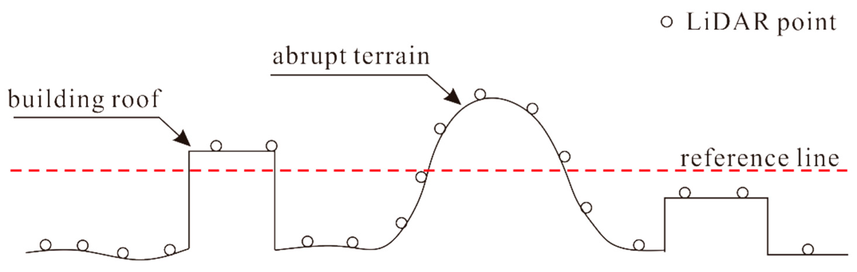
Although skewness balancing can obtain a promising filtering result in flat areas, it will cause a larger omission error in abrupt terrain. This effect is because there is an implicit assumption for skewness balancing that all ground points are located above the objects. However, this assumption is obviously unreasonable in undulating areas, such as mountains, cliffs, and ridges. As shown in Figure 4, some ground points are higher than some nonground points (building roof) in abrupt terrain environments. Thus, according to the principle of the skewness balancing, those ground points with higher elevations will be misclassified as nonground points. Meanwhile, due to the undulations of the ground, some nonground points with lower elevations will also be accepted as ground points. Therefore, the classical skewness balancing algorithm cannot perform well in these kinds of areas.
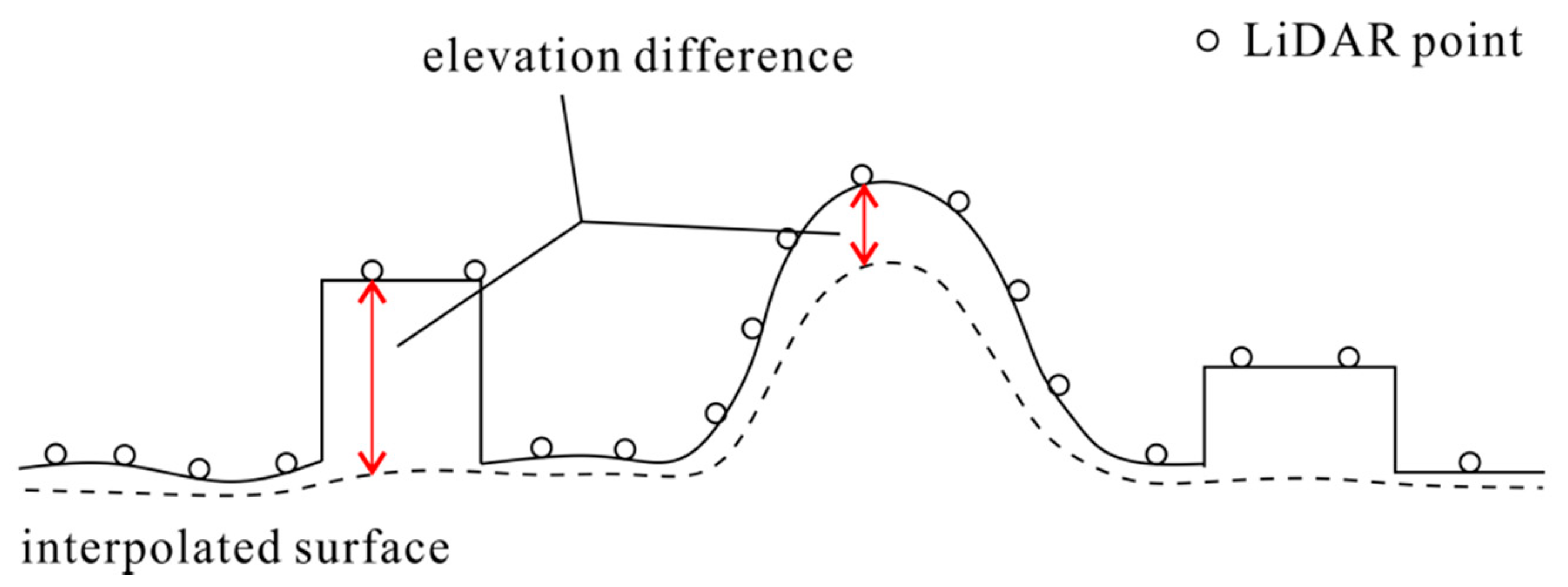
As shown in Figure 5, although both ground points and nonground points have elevation jumps, that effect will be changed if we build an interpolated surface based on the ground seeds. The ground seeds are points with the lowest elevations in local areas. Thus, the interpolated surface can reflect the fluctuation of the terrain. Although the elevations of some ground points are higher than those of nonground points, their corresponding elevation differences to the interpolated surface are totally different.
As shown in Figure 5, it is easy to find that the elevation differences between the ground points and the interpolated surface are obviously smaller than the elevation differences between the nonground points and the interpolated surface. This finding can avoid the misclassification of ground points and nonground points in undulating terrains. Thus, the improved method can be realized by modifying Equation (3) as:
where is the elevation difference of each point to the interpolated surface, and is the interpolated elevation of each point.
The key procedures for realizing the improved method are ground seed selection and interpolated surface construction. Ground seeds are the points with the lowest elevations and can be selected using pseudo-grids as presented in the Section 2.1. Note that the cell size used here should be larger than the largest size of an object. As such, we can guarantee that the seeds are true ground points. A thin plate spline (TPS) was adopted to build the interpolated surface, since it can produce smooth, oscillation-free surface [40]. Moreover, in comparison with the other three interpolation methods, namely, ordinary Kriging, inverse distance weighting, and triangular irregular network, the TPS performs the best for fitting the LiDAR data and is the only interpolator that does not erode the ground surface [41]. For a set of ground seeds , , the TPS can conduct interpolation to build a smooth surface , which is denoted as Equation (9):
where is a kernel function that is defined as , is the Euclidean distance, and column vector and can be estimated according to Equation (10):
where is a square matrix with a size of , is equal to , is an matrix with the -th row defined as , and is a tensor of the ground seeds.
The interpolated surface is obtained by minimizing the bending energy given by Equation (11) [42]. After obtaining the interpolated surface, of each point can be calculated easily.
3. Experimental Results
To evaluate the performance of the proposed method, the datasets provided by the ISPRS Commission III were employed [43]. The datasets are selected from seven sites located in the Vaihingen/Enz test field and Stuttgart city center. This paper chose one sample datum from each site. These selected samples (samp12, samp21, samp31, samp41, samp54, samp61 and samp71) cover different terrain features as shown in Table 1. These samples were classified correctly using semiautomatic filtering and subsequent manual editing. Thus, these samples are convenient for performing quantitative calculations.
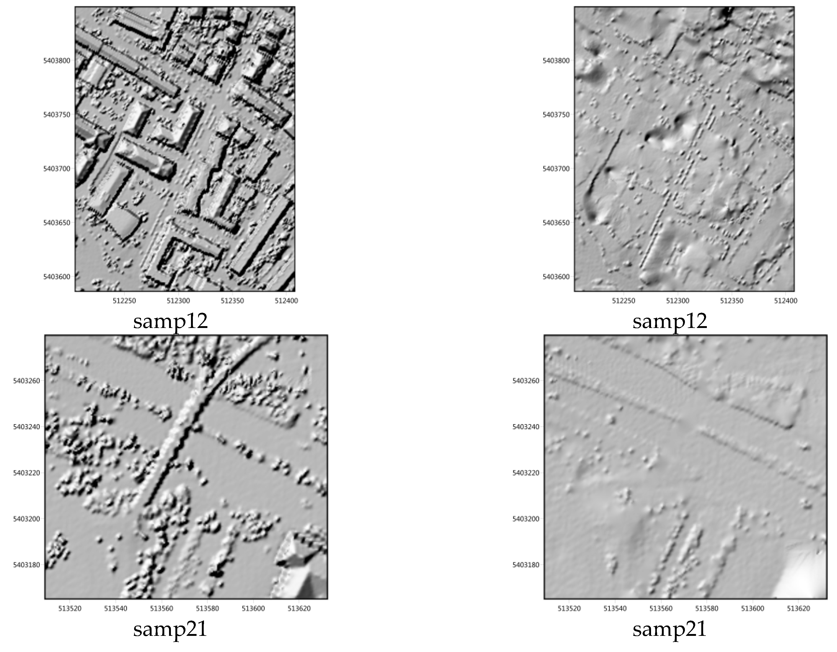
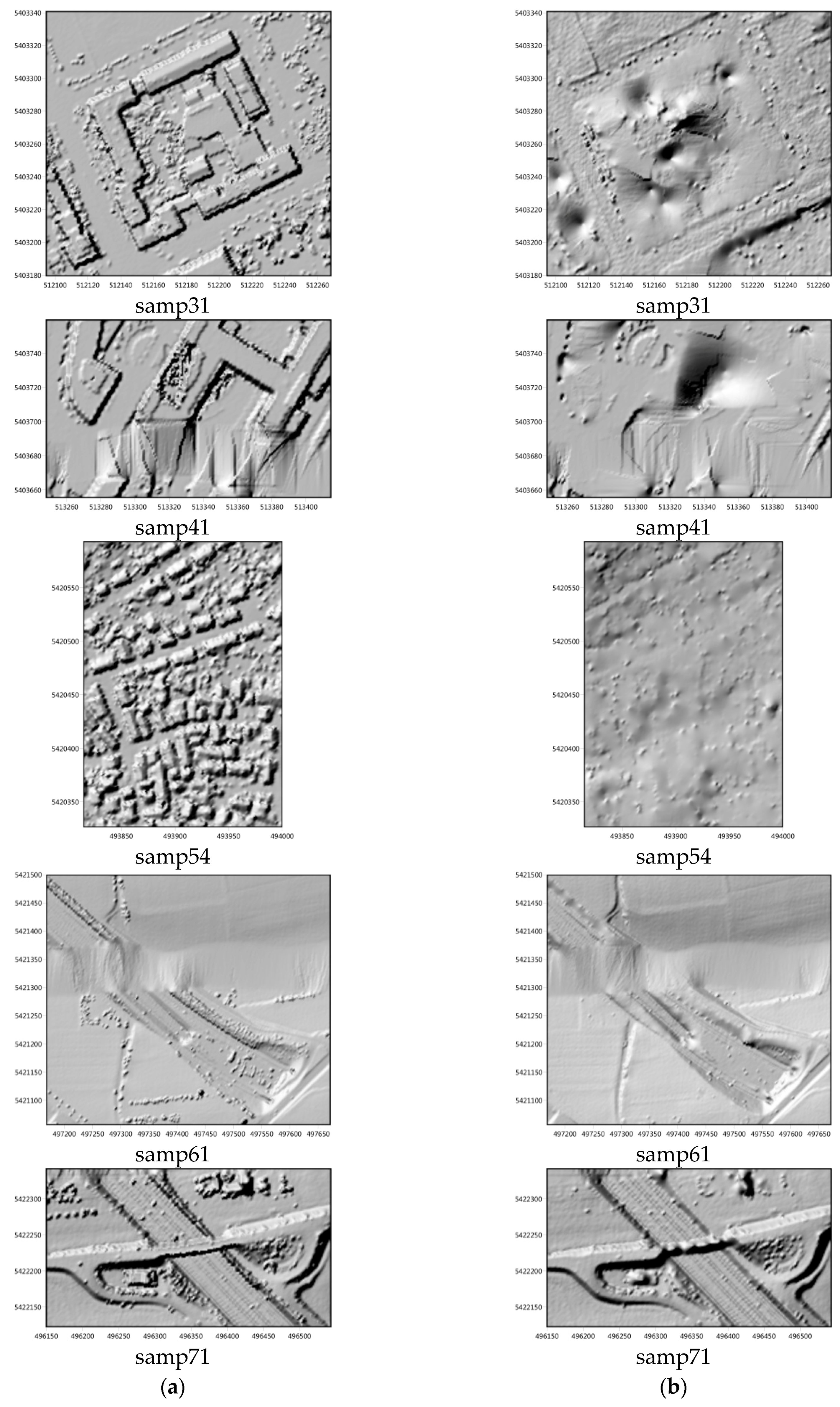
The filtering results of the seven samples are shown in Figure 6. Three accuracy metrics, namely Type I error, Type II error, and total error, are were adopted for the quantitative analysis. The Type I error is the proportion of ground points misclassified as nonground points, while the Type II error is the proportion of nonground points that the method fails to reject. The total error is the entire set of erroneous points. The filtering accuracy of the proposed method is shown in Table 2. In terms of the total error, the proposed method performs the best for samp21. Moreover, samp21 also has the smallest Type I error, which means that almost all the ground points are correctly classified. From samp12 (a) and samp12 (b) in Figure 6, it can be observed that the terrain in this sample is not too complicated. The main filtering challenge is the bridge, which has been removed effectively. Samp41 has the largest total error since both its Type I error and Type II error are larger. In the area of samp41, there are some complex buildings and low outliers. In particular, certain low outliers are dense enough to be hard to remove. These points are wrongly selected as ground seeds, which affects the accuracy of the interpolated surface. Therefore, the proposed method does not perform well in this area. From Table 2, it can be concluded that the proposed method is biased in favor of minimizing Type I errors because the average Type II error (9.94%) is more than two times the average Type I error (4.17%). That result occurs because samp71 and samp41 have larger Type II errors. Because Type II errors are easily modified, most filtering algorithms tend to suppress Type I errors at the expense of larger Type II errors.
4. Discussion
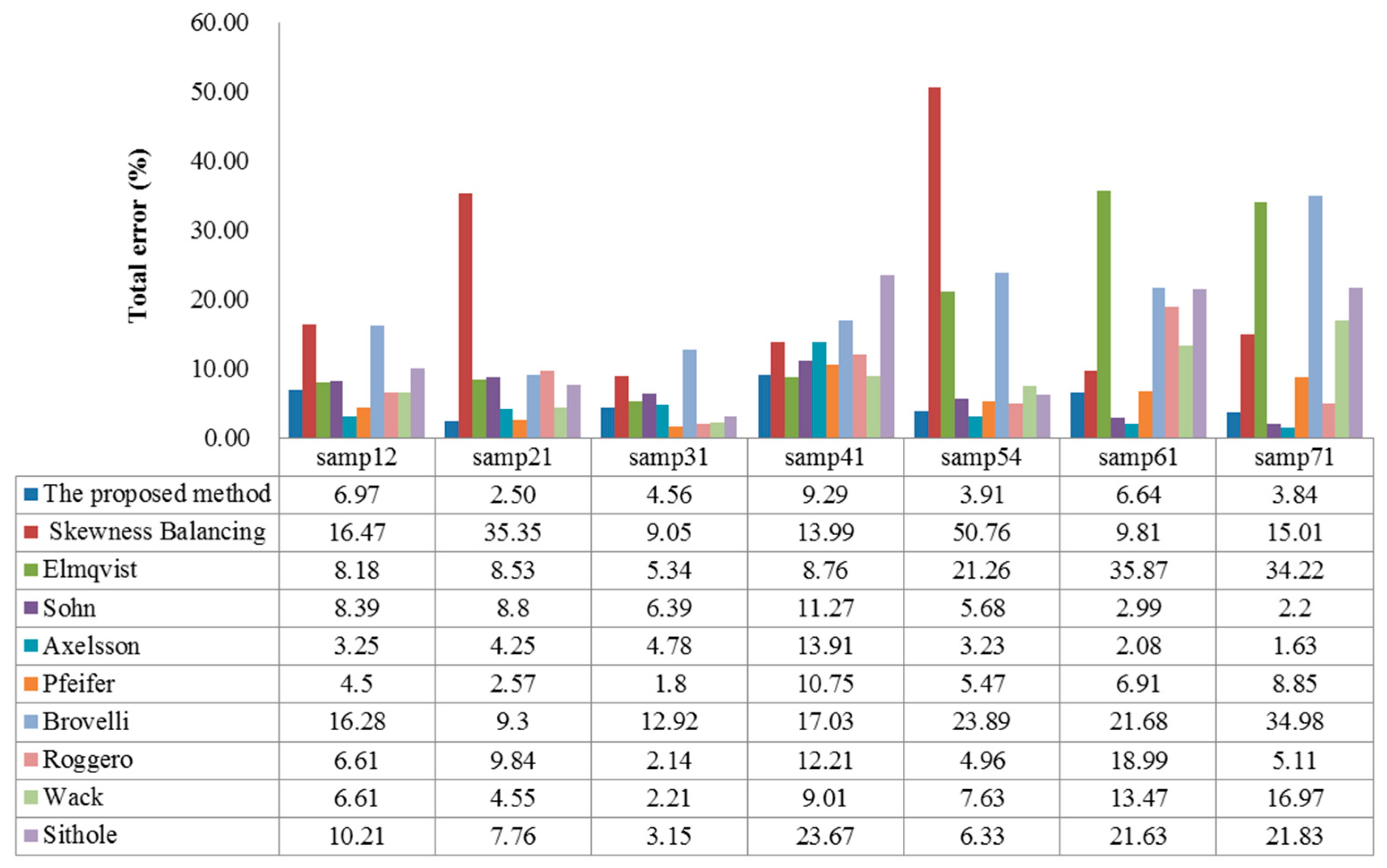
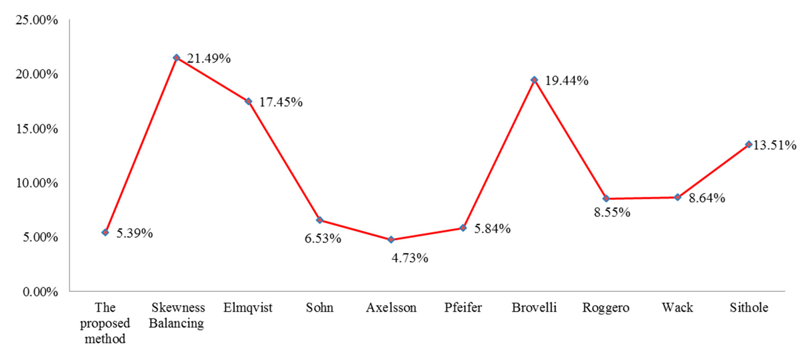
To objectively evaluate the performance of the proposed method, this paper compared the total errors of the proposed method to the classic skewness balancing method and eight other algorithms tested by the ISPRS [44]. As shown in Figure 7 and Figure 8, the improved method proposed in this paper performs much better than the classic skewness balancing method. The total errors of the seven samples are all smaller than those of skewness balancing. As a result, the average total error of the proposed method is much smaller than that of skewness balancing. Figure 8 shows that the proposed method outperforms most of the previous filtering methods except for the progressive triangulated irregular network densification (PTD) method proposed by Axelsson. The average total error of the proposed method is only slightly larger than that of the PTD method. Considering that the PTD method involves complex parameter settings, such as thresholds of iteration angle and distance, the proposed method has the advantage of a high degree of automation with satisfying filtering accuracy.
In recent years, some other modified filtering methods have also been proposed to improve filtering performance. Li et al. [4] proposed an improved morphological filtering method based on geodesic transformations of mathematical morphology. In their method, it is unnecessary to select different window sizes or determine the maximum window size. Thus, the robustness and automation of the morphological filtering method can be enhanced. Li et al. [5] put forward an improved top-hat filtering with sloped brim to extract ground points. To suppress the omission error caused by protruding terrain features, Li et al. [5] inspected the elevation change intensity of the transitions between the obtained top-hats and outer brims. In doing so, the filtering performance of the method towards various terrain environments can be improved. Most traditional morphology-based algorithms have difficulties in protecting terrain details, especially when using larger filtering windows. To solve this problem, Hui et al. [7] first proposed a hybrid filtering model that combines a traditional morphology-based filter and an interpolation-based filter. The morphological filters removed the nonground points with filtering window gradually downsizing. Meanwhile, Kriging interpolation is adopted based on the corresponding filtering windows. The experimental results show that the improved method has a significant advantage in protecting terrain details, thereby providing good filtering performance. Lin and Zhang [29] improved the classic progressive TIN (triangular irregular network) densification (PTD) method based on segmentation. In their method, point clouds are first segmented by region growing. Then, each terrain segment is added to the TIN iteratively. In so doing, the improved method can achieve a smaller omission error and total error than the traditional PTD method.
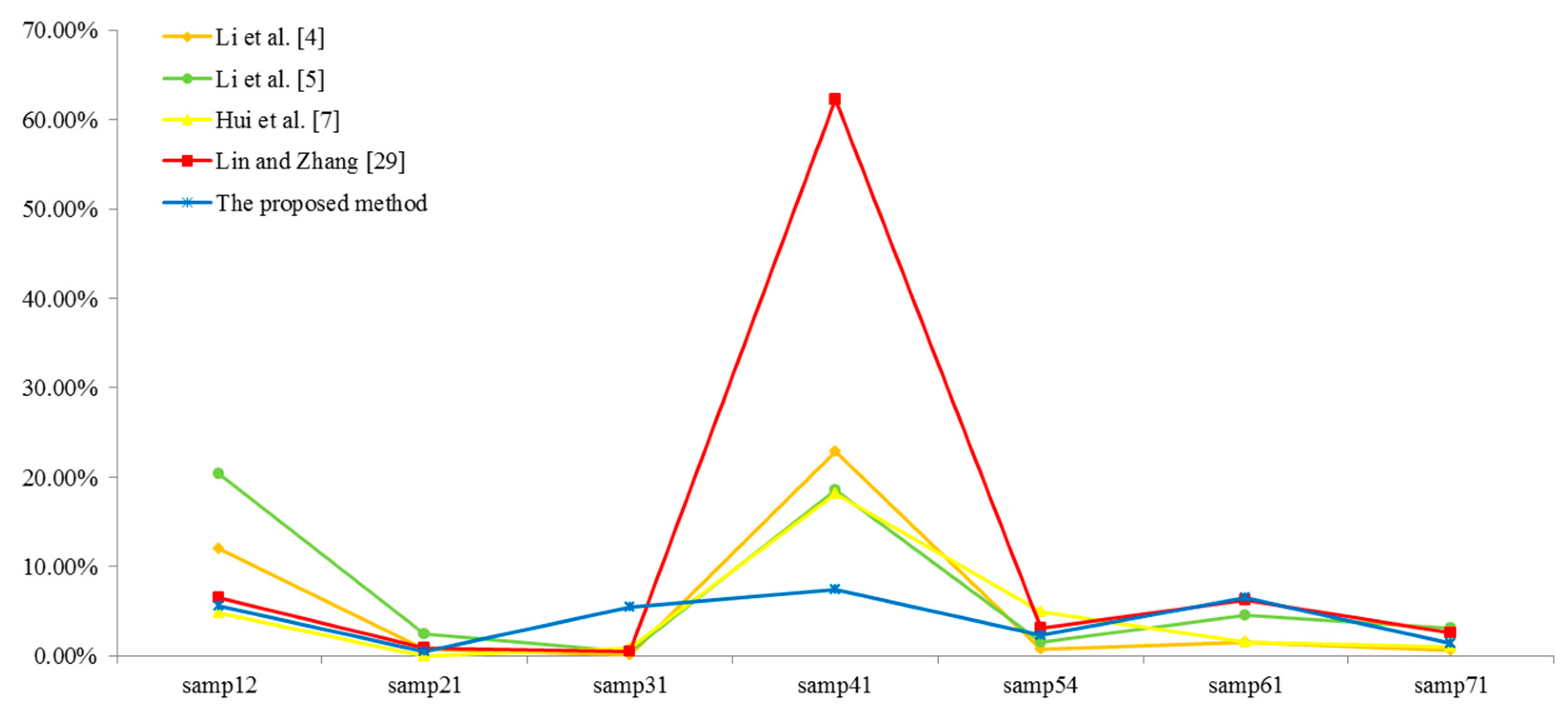
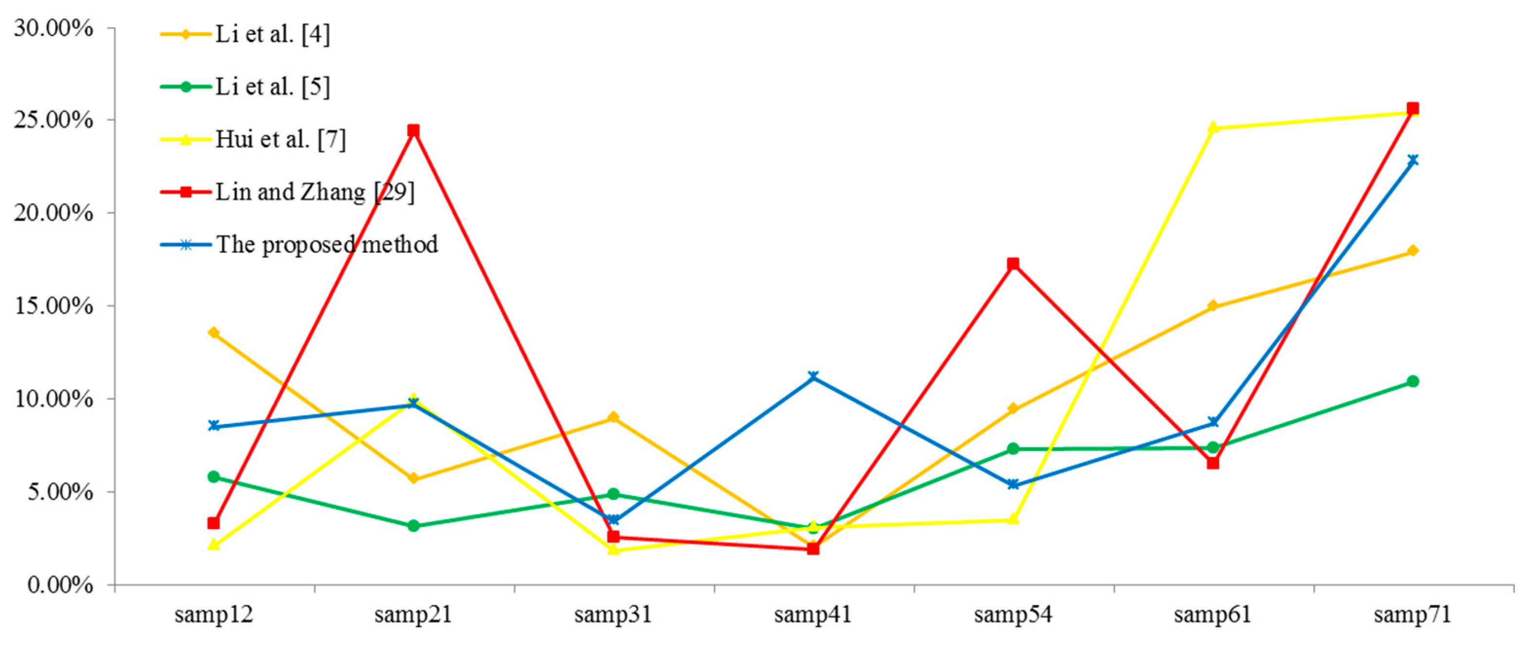
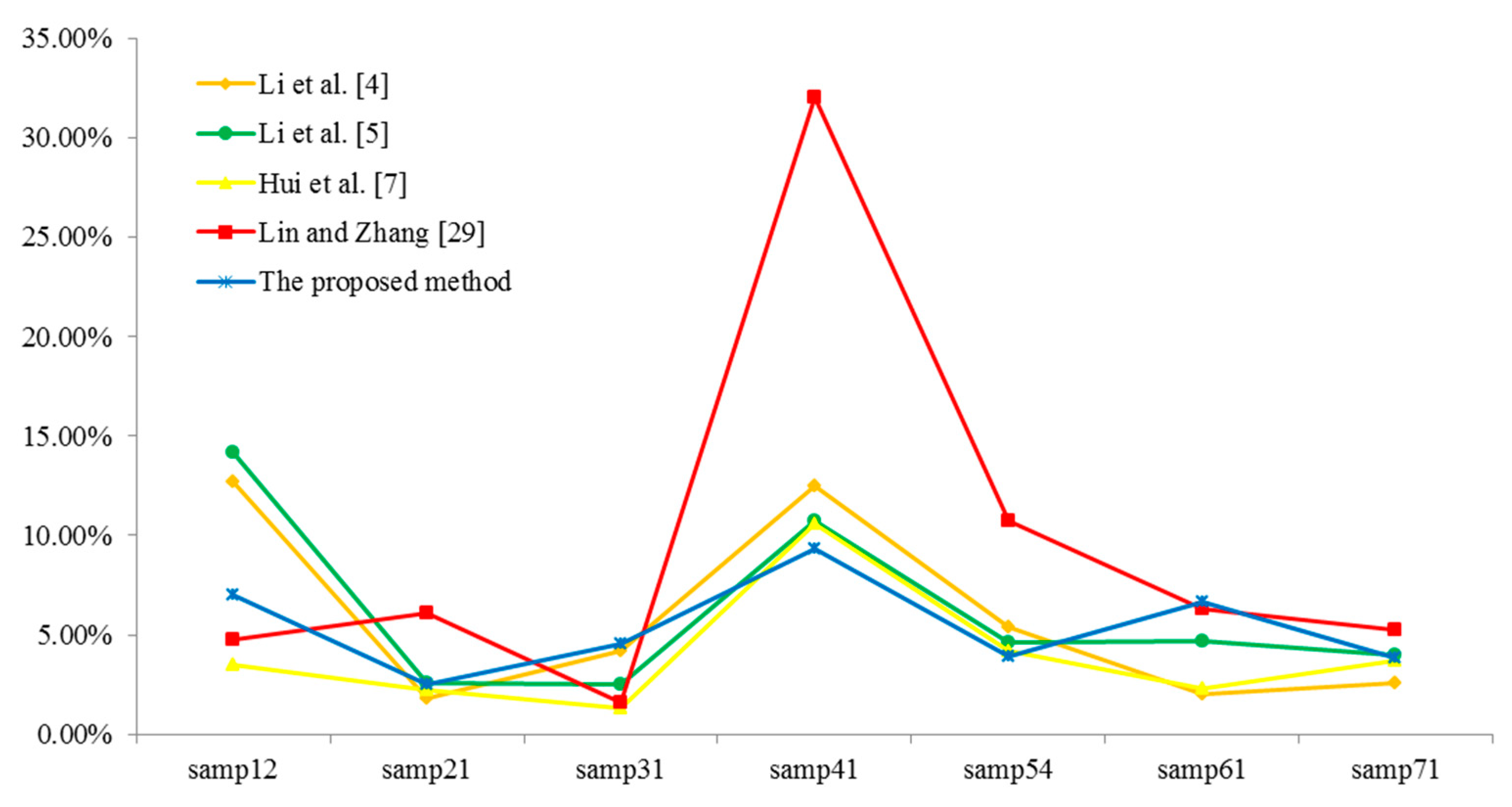
All the above-mentioned methods evaluate the filtering performance using the data sets provided by the ISPRS. This paper compares the type I error, type II error, and total error with those of the other four methods, as shown in Figure 9, Figure 10 and Figure 11. From Figure 9, it can be found that the proposed method achieved smaller type I errors than most of other methods, especially for samp41. As a result, in terms of average type I error, the proposed method performs the best. From Figure 10, it can be observed that almost all the methods have a larger type II error for samp71. This result is because there are many small low objects with similar elevations to the terrain in samp71. These objects are easily misclassified as ground points. Moreover, we can also find that the type II errors of the proposed method are slightly larger. Although the proposed method modified the classical skewness balancing algorithm using TPS interpolation, some nonground objects with low elevations are still easily misclassified as ground. In terms of the total error, as shown in Figure 11, this paper also outperforms the methods proposed by Li et al. [4], Li et al. [5], and Lin and Zhang [29]. Furthermore, the total errors of the seven samples do not change much. Thus, we can conclude that the proposed method can achieve good performance in various terrain environments.
5. Conclusions
Diverse changing terrain environments and complex parameter settings pose great challenges to airborne LiDAR filtering. To improve the accuracy and automation of the filtering method, this paper proposed an improved skewness balancing filtering algorithm based on thin plate spline interpolation. Our experiments indicate that the proposed method can achieve good filtering performance without parameter settings. Thus, this method can be easily applied by inexperienced researchers. In comparison with the other eight filtering methods tested by the ISPRS, the proposed method also outperforms most of these methods. Although the average total error of the proposed method is slightly larger than that of the PTD method proposed by Axelsson, the proposed method has a high degree of automation. Furthermore, this paper also compared the results of some other recently proposed improved methods. The comparisons indicate that the proposed method in this paper can achieve the smallest type I error. Thus, a better DTM can be generated using the filtering result since there are fewer non-ground points that are misclassified. Moreover, the total errors for the seven samples are also small. Therefore, the proposed method can achieve promising and comparable performance when faced with diverse landscapes. However, the Type II error of the proposed method is slightly larger. Especially in areas with complex objects, the proposed method may erroneously accept some nonground points as ground points. This problem can be overcome by cooperating with segmentation methods in future research.
Author Contributions
Z.H. had the original idea for the study. P.C. drafted the manuscript. Z.H. and Y.Y.Z. contributed to improvement of the original idea and revision of the manuscript. Y.X., Y.H. and J.W. performed the experiments and experimental analysis.
Funding
This research was funded by The National Key Research and Development Program of China (2017YFB0503704), National Science Foundation (NSF) (41801325, 41861052, 41601416), Education Department of Jiangxi Province (GJJ170449), Key Laboratory for Digital Land and Resources of Jiangxi Province, East China University of Technology (DLLJ201806), East China University of Technology Ph.D. Project (DHBK2017155) and the Spark planning project of Jiangxi Province (20161BBB29002), Key Laboratory of Watershed Ecology and Geographical Environment Monitoring, NASG (WE2016006).
Acknowledgments
The authors express their appreciation to the anonymous reviewers for their valuable suggestions.
Conflicts of Interest
The authors declare no conflict of interest.
References
- Filin, S.; Pfeifer, N. Segmentation of airborne laser scanning data using a slope adaptive neighborhood. ISPRS J. Photogramm. 2006, 60, 71–80. [Google Scholar] [CrossRef]
- Chen, Z.; Gao, B.; Devereux, B. State-of-the-Art: DTM Generation Using Airborne LIDAR Data. Sensors 2017, 17, 150. [Google Scholar] [CrossRef] [PubMed]
- Yang, B.; Huang, R.; Dong, Z.; Zang, Y.; Li, J. Two-step adaptive extraction method for ground points and breaklines from lidar point clouds. ISPRS J. Photogramm. 2016, 119, 373–389. [Google Scholar] [CrossRef]
- Li, Y.; Yong, B.; Oosterom, P.V.; Lemmens, M.; Wu, H.; Ren, L.; Zheng, M.; Zhou, J. Airborne LiDAR Data Filtering Based on Geodesic Transformations of Mathematical Morphology. Remote Sens. 2017, 9, 1104. [Google Scholar] [CrossRef]
- Li, Y.; Yong, B.; Wu, H.; An, R.; Xu, H. An Improved Top-Hat Filter with Sloped Brim for Extracting Ground Points from Airborne Lidar Point Clouds. Remote Sens. 2014, 6, 12885–12908. [Google Scholar] [CrossRef] [Green Version]
- Meng, X.; Currit, N.; Zhao, K. Ground Filtering Algorithms for Airborne LiDAR Data: A Review of Critical Issues. Remote Sens. 2010, 2, 833–860. [Google Scholar] [CrossRef] [Green Version]
- Hui, Z.; Hu, Y.; Yevenyo, Y.Z.; Yu, X. An Improved Morphological Algorithm for Filtering Airborne LiDAR Point Cloud Based on Multi-Level Kriging Interpolation. Remote Sens. 2016, 8, 35. [Google Scholar] [CrossRef]
- Zhou, G.; Zhou, X. Seamless Fusion of LiDAR and Aerial Imagery for Building Extraction. IEEE Trans. Geosci. Remote Sens. 2014, 52, 7393–7407. [Google Scholar] [CrossRef]
- Yang, B.; Huang, R.; Li, J.; Tian, M.; Dai, W.; Zhong, R. Automated Reconstruction of Building LoDs from Airborne LiDAR Point Clouds Using an Improved Morphological Scale Space. Remote Sens. 2016, 9, 14. [Google Scholar] [CrossRef]
- Xie, X.; Liu, Z.; Xu, C.; Zhang, Y. A Multiple Sensors Platform Method for Power Line Inspection Based on a Large Unmanned Helicopter. Sensors 2017, 17, 1222. [Google Scholar] [CrossRef]
- Qin, R. Change detection on LOD 2 building models with very high resolution spaceborne stereo imagery. ISPRS J. Photogramm. 2014, 96, 179–192. [Google Scholar] [CrossRef]
- Yan, W.Y.; Shaker, A.; El-Ashmawy, N. Urban land cover classification using airborne LiDAR data: A review. Remote Sens. Environ. 2015, 158, 295–310. [Google Scholar] [CrossRef]
- Sampath, A. Urban DEM Generation from Raw Lidar Data: A Labeling Algorithm and its Performance. Photogramm. Eng. Remote Sens. 2015, 71, 217–226. [Google Scholar]
- Vosselman, G. Slope based filtering of laser altimetry data. Int. Arch. Photogramm. Remote Sens. Spat. Inf. Sci. 2000, 33, 935–942. [Google Scholar]
- Sithole, G. Filtering of Laser Altimetry Data Using a Slope Adaptive Filter. Int. Arch. Photogramm. Remote Sens. 2001, 34, 203–210. [Google Scholar]
- Wang, C.K.; Tseng, Y.H. DEM gemeration from airborne lidar data by an adaptive dualdirectional slope filter. Int. Arch. Photogramm. Remote Sens. Spat. Inf. Sci. 2010, 38, 628–632. [Google Scholar]
- Susaki, J. Adaptive Slope Filtering of Airborne LiDAR Data in Urban Areas for Digital Terrain Model (DTM) Generation. Remote Sens. 2012, 4, 1804–1819. [Google Scholar] [CrossRef] [Green Version]
- Chen, Q.; Gong, P.; Baldocchi, D.; Xie, G. Filtering Airborne Laser Scanning Data with Morphological Methods. Photogramm. Eng. Remote Sens. 2007, 73, 175–185. [Google Scholar] [CrossRef]
- Li, Y.; Wu, H.; Xu, H.; An, R.; Xu, J.; He, Q. A gradient-constrained morphological filtering algorithm for airborne LiDAR. Opt. Laser Technol. 2013, 54, 288–296. [Google Scholar] [CrossRef]
- Li, Y.; Yong, B.; Wu, H.; An, R.; Xu, H.; Xu, J.; He, Q. Filtering Airborne Lidar Data by Modified White Top-Hat Transform with Directional Edge Constraints. Photogramm. Eng. Remote Sens. 2014, 80, 133–141. [Google Scholar] [CrossRef]
- Mongus, D.; Lukač, N.; Žalik, B. Ground and building extraction from LiDAR data based on differential morphological profiles and locally fitted surfaces. ISPRS J. Photogramm. 2014, 93, 145–156. [Google Scholar] [CrossRef]
- Pingel, T.J.; Clarke, K.C.; McBride, W.A. An improved simple morphological filter for the terrain classification of airborne LIDAR data. ISPRS J. Photogramm. 2013, 77, 21–30. [Google Scholar] [CrossRef]
- Zhang, K.Q.; Chen, S.C.; Whitman, D.; Shyu, M.L.; Yan, J.H.; Zhang, C.C. A progressive morphological filter for removing nonground measurements from airborne LIDAR data. IEEE Trans. Geosci. Remote Sens. 2003, 41, 872–882. [Google Scholar] [CrossRef] [Green Version]
- Axelsson, P. DEM generation from laser scanner data using adaptive TIN models. Int. Arch. Photogramm. Remote Sens. Spat. Inf. Sci. 2000, 33, 110–117. [Google Scholar]
- Zhang, J.; Lin, X. Filtering airborne LiDAR data by embedding smoothness-constrained segmentation in progressive TIN densification. ISPRS J. Photogramm. 2013, 81, 44–59. [Google Scholar] [CrossRef]
- Zhao, X.; Guo, Q.; Su, Y.; Xue, B. Improved progressive TIN densification filtering algorithm for airborne LiDAR data in forested areas. ISPRS J. Photogramm. 2016, 117, 79–91. [Google Scholar] [CrossRef] [Green Version]
- Wang, H.; Wang, S.; Chen, Q.; Jin, W.; Sun, M. An improved filter of progressive TIN densification for LiDAR point cloud data. Wuhan Univ. J. Nat. Sci. 2015, 20, 362–368. [Google Scholar] [CrossRef]
- Tóvári, D.; Pfeifer, N. Segmentation based robust interpolation–a new approach to laser data filtering. Int. Arch. Photogramm. Remote Sens. Spat. Inf. Sci. 2005, 36, 79–84. [Google Scholar]
- Lin, X.; Zhang, J. Segmentation-Based Filtering of Airborne LiDAR Point Clouds by Progressive Densification of Terrain Segments. Remote Sens. 2014, 6, 1294–1326. [Google Scholar] [CrossRef] [Green Version]
- Chen, C.; Li, Y.; Yan, C.; Dai, H.; Liu, G.; Guo, J. An improved multi-resolution hierarchical classification method based on robust segmentation for filtering ALS point clouds. Int. J. Remote Sens. 2016, 37, 950–968. [Google Scholar] [CrossRef]
- Kraus, K.; Pfeifer, N. Determination of terrain models in wooded areas with airborne laser scanner data. ISPRS J. Photogramm. Remote Sens. 1998, 53, 193–203. [Google Scholar] [CrossRef]
- Rodríguez-Caballero, E.; Afana, A.; Chamizo, S.; Solé-Benet, S.; Solé-Benet, A.; Canton, Y. A new adaptive method to filter terrestrial laser scanner point clouds using morphological filters and spectral information to conserve surface micro-topography. ISPRS J. Photogramm. Remote Sens. 2016, 117, 141–148. [Google Scholar] [CrossRef]
- Che, E.; Olsen, M. Fast ground filtering for TLS data via scanline density analysis. ISPRS J. Photogramm. Remote Sens. 2017, 129, 226–240. [Google Scholar] [CrossRef]
- Wu, B.; Yu, B.; Huang, C.; Wu, Q.; Wu, J. Automated extraction of ground surface along urban roads from mobile laser scanning point clouds. Remote Sens. Lett. 2016, 7, 170–179. [Google Scholar] [CrossRef]
- Yan, L.; Liu, H.; Tan, J.; Li, Z.; Chen, C. A multi-constraint combined method for ground surface point filtering from mobile LiDAR point clouds. Remote Sens. 2017, 9, 958. [Google Scholar]
- Bartels, M.; Wei, H.; Mason, D.C. DTM generation from LIDAR data using Skewness Balancing. In Proceedings of the 18th International Conference on Pattern Recognition I, Hong Kong, China, 20–24 August 2006; pp. 566–569. [Google Scholar]
- Zeng, Z.; Wan, J.; Liu, H. An entropy-based filtering approach for airborne laser scanning data. Infrared Phys. Technol. 2016, 75, 87–92. [Google Scholar] [CrossRef]
- Duda, R.O.; Hart, P.E.; Stork, D.G. Pattern Classification; Wiley: Hoboken, NJ, USA, 1973. [Google Scholar]
- Bartels, M.; Wei, H. Threshold-free object and ground point separation in LIDAR data. Pattern Recognit. Lett. 2010, 31, 1089–1099. [Google Scholar] [CrossRef]
- Mongus, D.; Žalik, B. Parameter-free ground filtering of LiDAR data for automatic DTM generation. ISPRS J. Photogramm. 2012, 67, 1–12. [Google Scholar] [CrossRef]
- Evans, J.S.; Hudak, A.T. A Multiscale Curvature Algorithm for Classifying Discrete Return LiDAR in Forested Environments. IEEE Trans. Geosci. Remote Sens. 2007, 45, 1029–1038. [Google Scholar] [CrossRef] [Green Version]
- Zandifar, A.; Lim, S.; Duraiswami, R.; Gumerov, N.A.; Davis, L.S. Multi-level fast multipole method for thin plate spline evaluation. In Proceedings of the 2004 International Conference on Image Processing, Singapore, 24–27 October 2004; pp. 1683–1686. [Google Scholar]
- Datasets Provided by the ISPRS Commission III. Available online: http://www.itc.nl/isprswgIII-3/filtertest/ (accessed on 8 January 2018).
- Sithole, G.; Vosselman, G. Report: ISPRS Comparison of Filters; Delft University of Technology: Delft, The Netherlands, 2003. [Google Scholar]
Figure 1.
A horizontal profile of the digital surface model (DSM) generated using raw light detection and ranging (LiDAR) point clouds without denoising.
Figure 1.
A horizontal profile of the digital surface model (DSM) generated using raw light detection and ranging (LiDAR) point clouds without denoising.

Figure 2.
Pseudo grids construction for point clouds.

Figure 3.
Sketch map of the structure element.

Figure 4.
Undulation terrains with ground points located above objects.

Figure 5.
Principle of the improved method.

Figure 6.
Filtering results: (a) the DSMs before filtering; (b) the filtered DEMs generated from the ground points derived by the proposed filtering algorithm.
Figure 6.
Filtering results: (a) the DSMs before filtering; (b) the filtered DEMs generated from the ground points derived by the proposed filtering algorithm.


Figure 7.
Comparison of total errors of the proposed method and previous filtering methods.

Figure 8.
Comparison of average total error of the proposed method and previous filtering methods.

Figure 9.
Comparison of type I errors of other four improved filters for the seven samples.

Figure 10.
Comparison of type II errors of other four improved filters for the seven samples.

Figure 11.
Comparison of total errors of other four improved filters for the seven samples.


Table 1.
Terrain features of the selected seven samples.
| Samples | Terrain Features |
|---|---|
| samp12 | Small objects, mixed vegetation and buildings |
| samp21 | Attached objects, narrow bridge, and low vegetation |
| samp31 | Dense buildings, data gaps, and mixture of high and low objects |
| samp41 | Data gaps, complex buildings, and low outliers |
| samp54 | Gentle sloped terrains, dense objects |
| samp61 | Buildings, embankments, data gaps, and roads |
| samp71 | Bridges, embankments, underpasses, and roads |
Table 2.
Accuracy indexes for the seven samples.
| Sample | The Proposed Method | ||
|---|---|---|---|
| Type I (%) | Type II (%) | Total (%) | |
| samp12 | 5.55 | 8.49 | 6.97 |
| samp21 | 0.47 | 9.65 | 2.50 |
| samp31 | 5.52 | 3.44 | 4.56 |
| samp41 | 7.43 | 11.14 | 9.29 |
| samp54 | 2.26 | 5.34 | 3.91 |
| samp61 | 6.57 | 8.71 | 6.64 |
| samp71 | 1.41 | 22.82 | 3.84 |
| Mean | 4.17 | 9.94 | 5.39 |
© 2019 by the authors. Licensee MDPI, Basel, Switzerland. This article is an open access article distributed under the terms and conditions of the Creative Commons Attribution (CC BY) license (http://creativecommons.org/licenses/by/4.0/).
Share and Cite
MDPI and ACS Style
Cheng, P.; Hui, Z.; Xia, Y.; Ziggah, Y.Y.; Hu, Y.; Wu, J. An Improved Skewness Balancing Filtering Algorithm Based on Thin Plate Spline Interpolation. Appl. Sci. 2019, 9, 203. https://0-doi-org.brum.beds.ac.uk/10.3390/app9010203
AMA Style
Cheng P, Hui Z, Xia Y, Ziggah YY, Hu Y, Wu J. An Improved Skewness Balancing Filtering Algorithm Based on Thin Plate Spline Interpolation. Applied Sciences. 2019; 9(1):203. https://0-doi-org.brum.beds.ac.uk/10.3390/app9010203
Chicago/Turabian StyleCheng, Penggen, Zhenyang Hui, Yuanping Xia, Yao Yevenyo Ziggah, Youjian Hu, and Jing Wu. 2019. "An Improved Skewness Balancing Filtering Algorithm Based on Thin Plate Spline Interpolation" Applied Sciences 9, no. 1: 203. https://0-doi-org.brum.beds.ac.uk/10.3390/app9010203
Note that from the first issue of 2016, this journal uses article numbers instead of page numbers. See further details here.