Investigation on Interference Test for Wells Connected by a Large Fracture


1
Institute of Mechanics, Chinese Academy of Sciences, Beijing 100190, China
2
School of Engineering Science, University of Chinese Academy of Sciences, Beijing 100049, China
3
School of Civil and Resource Engineering, University of Science and Technology Beijing, Beijing 100083, China
*
Authors to whom correspondence should be addressed.
Appl. Sci. 2019, 9(1), 206; https://0-doi-org.brum.beds.ac.uk/10.3390/app9010206
Submission received: 14 November 2018
/
Revised: 31 December 2018
/
Accepted: 3 January 2019
/
Published: 8 January 2019
Abstract
:Featured Application
Evaluate the connectivity of wells near the fault or connected by hydraulic fractures.
Abstract
Pressure communication between adjacent wells is frequently encountered in multi-stage hydraulic fractured shale gas reservoirs. An interference test is one of the most popular methods for testing the connectivity of a reservoir. Currently, there is no practical analysis model of an interference test for wells connected by large fractures. A one-dimensional equation of flow in porous media is established, and an analytical solution under the constant production rate is obtained using a similarity transformation. Based on this solution, the extremum equation of the interference test for wells connected by a large fracture is derived. The type-curve of pressure and the pressure derivative of an interference test of wells connected by a large fracture are plotted, and verified against interference test data. The extremum equation of wells connected by a large fracture differs from that for homogeneous reservoirs by a factor 2. Considering the difference of the flowing distance, it can be concluded that the pressure conductivity coefficient computed by the extremum equation of homogeneous reservoirs is accurate in the order of magnitude. On the double logarithmic type-curve, as time increases, the curves of pressure and the pressure derivative tend to be parallel straight lines with a slope of 0.5. When the crossflow of the reservoir matrix to the large fracture cannot be ignored, the slope of the parallel straight lines is 0.25. They are different from the type-curves of homogeneous and double porosity reservoirs. Therefore, the pressure derivative curve is proposed to diagnose the connection form of wells.
1. Introduction
The connectivity and permeable directivity of a reservoir are needed for the design of a development plan that accounts for such factors as a reasonable well pattern, the option of injection, and production wells for injection water or gas development [1,2,3,4,5]. The connectivity and permeable directivity are usually tested via interference test. The interference test is also widely used to investigate the properties of water and geothermal wells, except oil and gas wells [6,7].
Early in 1936, Theis [8] proposed the type-curve of the interference test for homogeneous reservoirs but did not account for the impact of the wellbore storage effect and the skin effect, which were later studied by Obge Brigham et al. [9]. In 1972, Gringarten and Witherspoon [10] presented the curves of the interference test for vertically fractured wells. An interference test analysis model for complex reservoirs, such as composite reservoirs [11], two-layered commingled reservoirs [12], and a deformable reservoir [13] have also been proposed. Martinez [14] proposed a method to distinguish the spherical flow and linear flow for the interference test. Since the 1990s, the interference test analysis model for horizontal wells has become a hot topic [15,16,17], such as the models for anisotropic horizontal wells [18,19], fractured horizontal wells [20], and multilayers horizontal wells [21,22].
The interference test can also be used to investigate the connectivity between an injection well and a production well, where interference test analysis models of a multiphase flow [23,24,25] are needed. Koening et al. [26] and Ajani et al. [27] studied interference test analysis models that consider complex flow mechanisms for unconventional reservoirs.
Most existing interference test analysis models consider homogeneous reservoirs with different boundaries, but most reservoirs are heterogeneous and have fractures. If the geological information is complete, a numerical interference test analysis can be performed for a heterogeneous reservoir. A fractured reservoir can be characterized by a multimedium model or discrete fracture model depending on the density of fractures. Kazemi and Deruyck analyzed the interference test of double porosity medium reservoirs using the Warren–Root model for reservoirs with intensive fractures [28,29,30]. The multimedium model does not work for reservoirs with sparse fractures. For example, the reservoirs at Halahatang Oilfield, Tarim Basin in China are occurrent along faults resembling a string of beads. Although Biryukov and Kuchuk [31] investigated the effect of discrete fractures on well test curves, there are few studies on the impact of large fractures on the interference test.
In the past decade, multi-stage hydraulic fracturing horizontal wells have been widely used in shale gas development. Frequently, hydraulic fracturing causes pressure communication in adjacent horizontal wells [32,33,34]. Interference test wells are also used to test their connectivity [35]. The existing analysis models consider the flow of the entire reservoir and are generally solved through numerical or semi-numerical methods [36,37]. However, it is not necessary to consider the matrix flow in a fractured reservoir when the test time is short.
Therefore, a one-dimensional equation of flow in porous media is presented in this paper to study the pressure transient of wells connected by large fractures. Using its solution, an extremum equation and interference test type-curve for wells connected by a large fracture (WsCLF) were obtained and compared with the type-curve of homogeneous reservoirs and double porosity reservoirs. The results were verified against interference test data.
2. Methodology
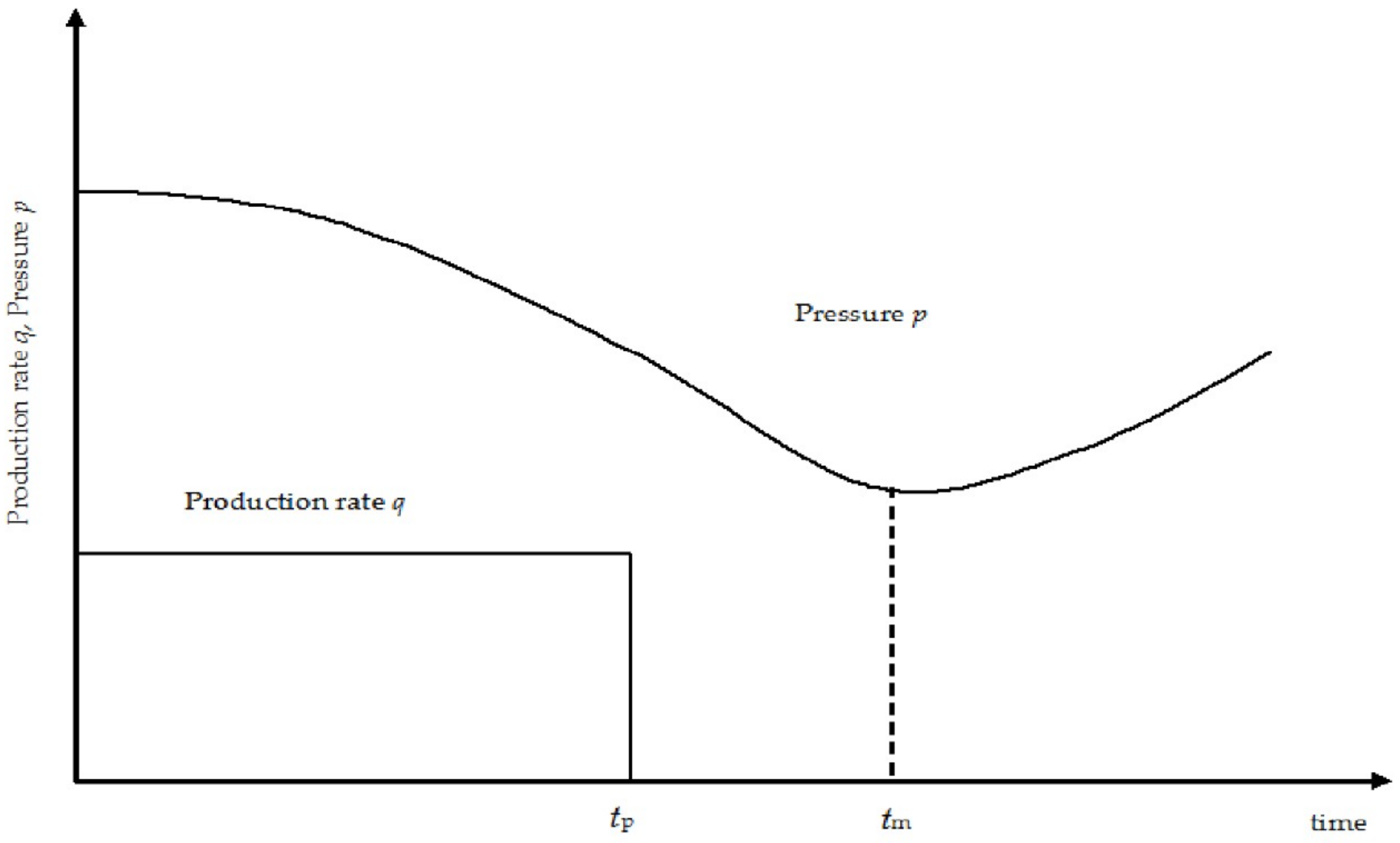
When an interference test is performed, a well is selected as an active well, and its production rate is changed to vary the pressure of the reservoir. At the same time, a neighboring well acts as an observation well, in which a high-precision pressure gauge is used to record the pressure variation. The production rate variation of the active well and the pressure in the observation well are shown in Figure 1. The connectivity is determined according to the pressure response in the observation well, and the pressure conductivity coefficient is calculated based on the time interval of the pressure signal received and other information [38].
3. Model and Solution for the Interference Test
3.1. Mathematical Model and Pressure Transient Solution
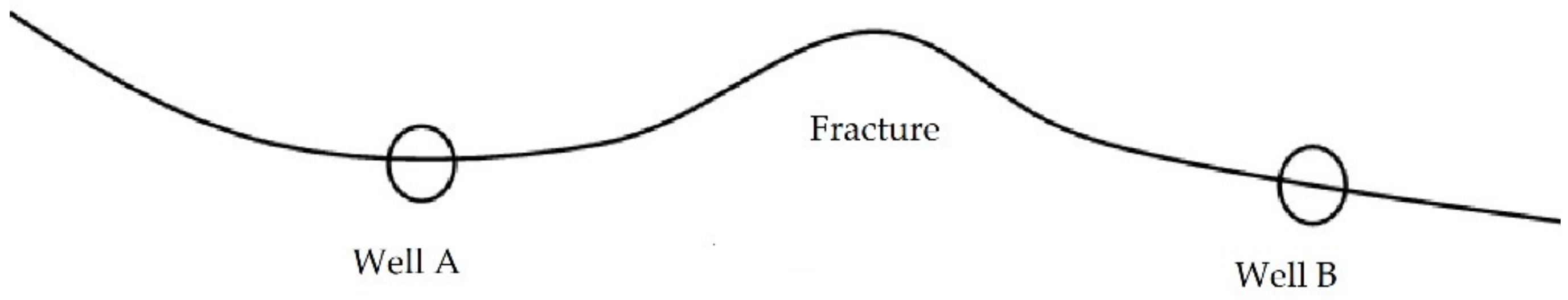
A simplified physical model considers two wells A and B connected by a large fracture. Well A is an active well, and it shuts in after a period of production time tp. Well B is an observation well, in which a precision pressure gauge is set up at the bottom-hole and kept closed. When the production time is short and the matrix of the reservoir is tight, well A and B influence each other mainly by the flow in large fractures, and the impact of flow in the matrix can be ignored. The fracture is presumed to run through the formation vertically. Therefore, the flow in the fracture can be treated as one-dimensional flow. The original of the coordinate system is set at Well A, and the right direction of axis x is along the fracture from Well A to Well B (Figure 2). The latter analysis assumes that the activation signal does not reach the end of the fracture which is treated as an infinite condition. The one-dimensional equation of flow in porous media is [39]
where p is the reservoir pressure (Pa), x is the coordinate along fracture (m), t is the time (s) and η is the pressure conductivity coefficient (m2/s).
Considering the pressure transient when Well A produces with a production rate q, boundary conditions and initial conditions are
where b is the fracture width (m), h is the reservoir thickness (m), K is the permeability of fracture (m2), B is the volumetric ratio of fluid, μ is the viscosity (Pa∙s), pi is the original pressure of reservoir, (Pa).
Defining the dimensionless quantities
The governing Equation (1) becomes Equation (6) [39]
The initial conditions and boundary condition Equations (2)–(4) can be written as Equations (7)–(9)
Given the above equations, the following similarity transformation is performed according to Liu et al. [39].
Then
Therefore, the governing equation becomes
and the boundary conditions and initial conditions are written as the following
A special solution of Equation (15) is
Assuming another special solution that is linearly independent with U1 is
Substituting Equation (19) into the control differential Equation (15)
Solving Equation (20), the following equation is derived
Therefore, another special solution is
The general solution is
where c1 and c2 are constant, and erf denotes the error function. Using the definite conditions Equations (16) and (17), the following constants are determined
Therefore, the solution of Equations (15) and (16) is
The solution of Equations (6)–(9) is
Transforming the solution into the dimensional form, the pressure transient of the well with the production q is
It can be seen from Equation (27) that the pressure change of the active well can immediately affect the pressure of the observation well. However, the pressure variation can only be observed when the pressure changes exceed the pressure gauge resolution and maximum noise.
3.2. Extremum Analysis of the Interference Test
When Well A shuts after a period of production time tp with a production rate q, the pressure transient of Well B can be derived by the superposition principle because the governing Equation (1) is a linear equation, as follows
To the pressure transient of Well B in the period (0, tp), the ratio of pressure change can be derived using Equation (26) as follows
Therefore, in the period (0, tp), the pressure of Well B is monotonically decreasing. When t > tp, according to Equation (27),
Setting
then
Using Equation (31), the following equation is derived
It can easily be found that when , f(t) monotonically increases, while when , f(t) monotonically decreases. Combining the above equation with Equation (32), it can be concluded that when , , the pressure p of Well B monotonically increases, and when , , the pressure p of well B monotonically decreases.
The continuously differentiable function p monotonically decreases in the region [0, max (tp, )], and monotonically increases in the region . Therefore, there must be a point when the pressure p of Well B reaches a minimal value. According to the extremum condition of a function,
where tm is the time when the pressure reaches the minimal value. From Equation (34), we can get the pressure conductivity coefficient as follows
3.3. Type-Curve of the Interference Test
The interference test type-curve can be obtained when the active well keeps producing and the observation well stays closed. The dimensionless pressure derivative can be defined similarly to that in the pressure transient analysis
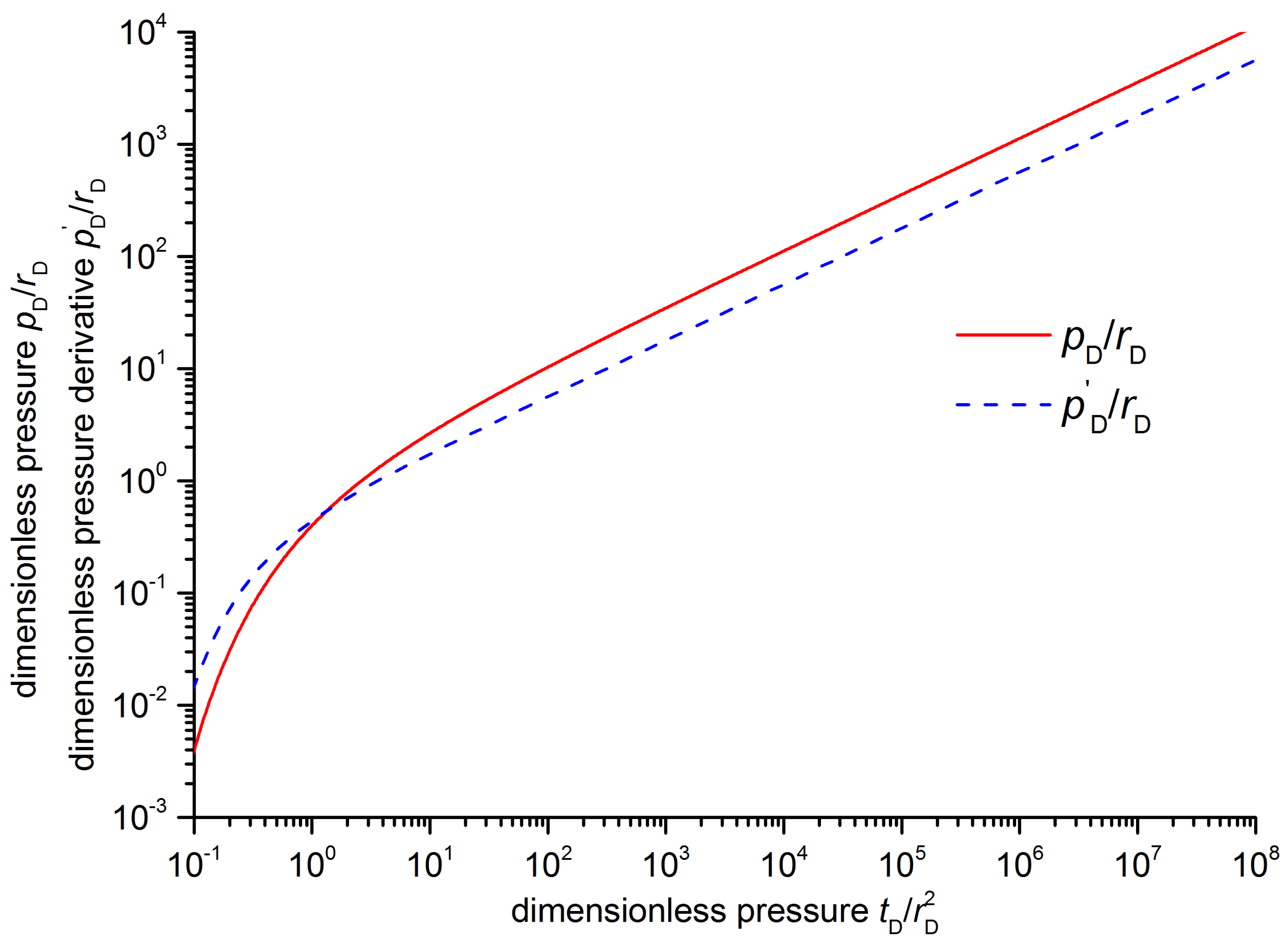
In Equation (36), the variable rD that replaces the variable xD is the distance between the active well and the observation well along the fracture. The curves of the dimensionless pressure derivative denoted in Equation (36) and the dimensionless pressure denoted in Equation (26) are drawn in one type-curve as Figure 3. This finding can be observed in the double logarithmic coordinate system, when the distance between wells is constant, the pressure and pressure derivative increase over time, and the speed of increase approaches a constant. Both of the two curves become linear with a slope of 0.5.
It is easy to obtain the cross point of a dimensionless pressure curve and dimensionless pressure derivative curve in an interference test type-curve of WsCLF as follows:
When , according to Equations (26) and (36), it can be found that
Therefore, approaches a straight line through the original point. However, in a homogeneous reservoir, pD~lgtD becomes a straight line when . In a double logarithmic coordinate system, it can also be found that
Thus, the distance between pD/rD and p′D/rD is lg2 log-period in a double-logarithmic coordinate system.
If the distance between wells and the width of the fracture are known, the pressure conductivity coefficient and permeability can be obtained by fitting the pressure and pressure derivative with the type-curve of interference test. Because it is difficult to obtain a precise value of the width of a fracture, the fracture conductivity Kb is usually computed.
4. Verification of the Interference Test Analysis Model for Wells Connected by a Large Fracture
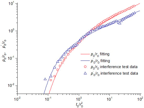
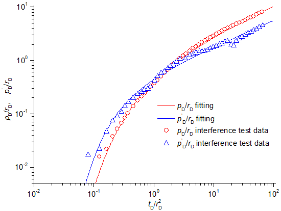
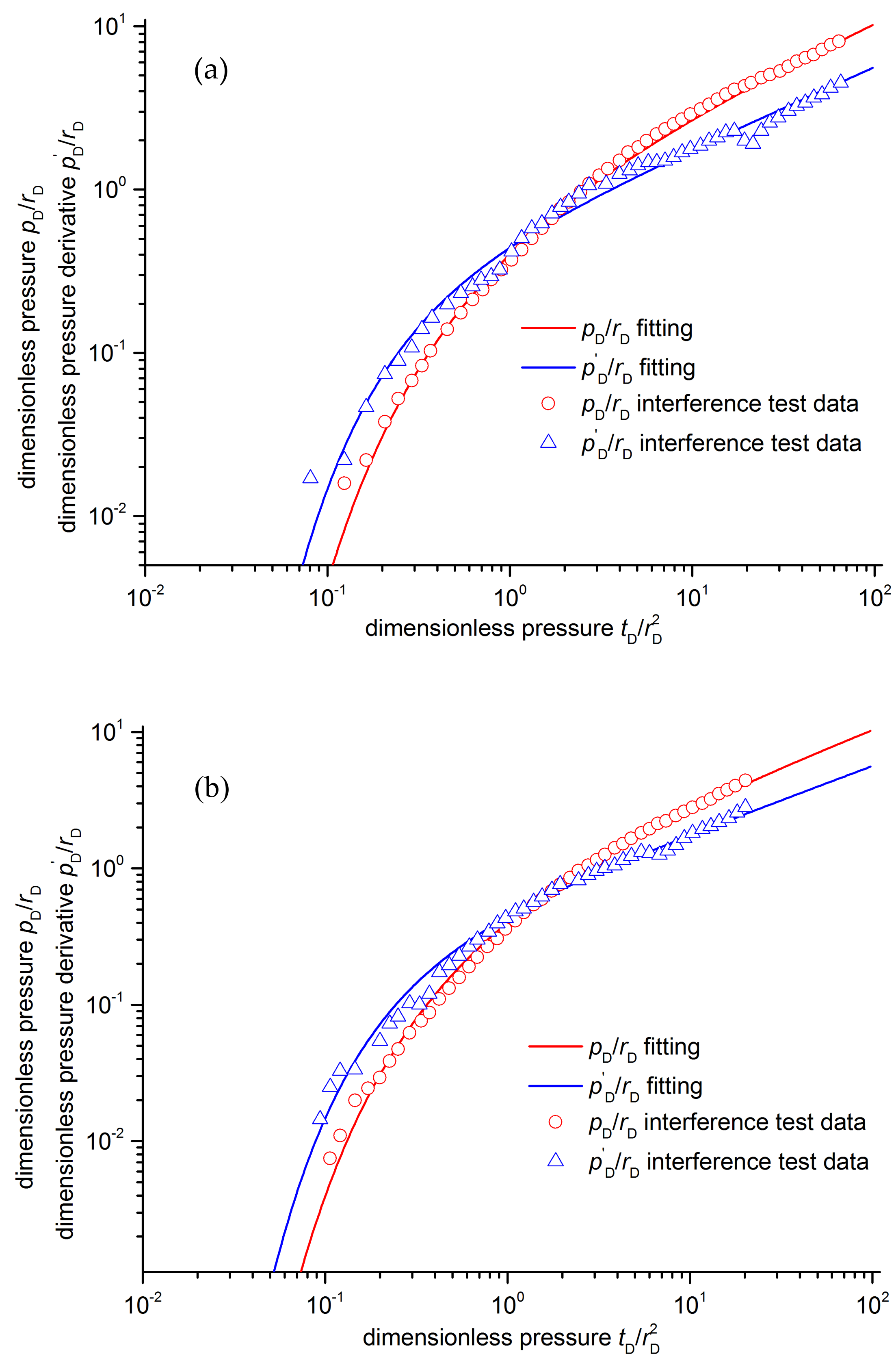
The previously proposed model was verified against interference test data from Chu et al. [36]. Due to the fracturing of the horizontal well, Chu et al. [36] found that the 3H well was connected to the 4H and 6H wells. Although they are horizontal wells and 3H and 4H wells are vertically connected, it is not difficult to understand that our model still applies. It can be seen that the fitting results are very good (Figure 4), and this proves the correctness of the proposed model. The fitting parameters for the 4H well are
where r is the distance between wells along the fracture (m). For the 6H well, the fitting parameters are
It should be noted that h in the above Equations (40) and (41) is not the thickness of the formation, but the width of the inter-well fracture communication. Since the production rate q, distance between wells r, viscosity μ, and volumetric ratio of fluid B are not given, and h is unknown, the permeability K and the pressure conductivity coefficient η cannot be further determined.
5. Discussion
The assumption that two wells are connected by a large fracture is usually too strong. Actually, they may be connected by the channel formed through several groups of intersected fractures. However, this does not influence the analysis process and results in this study. When one well connects with multiwells through several large fractures, it has little impact on the computation result of the pressure conductivity coefficient because the equation of the pressure conductivity coefficient derived by the extremum analysis is independent of the flow rate.
To further understand its characteristics, the interference test of WsCLF, is compared with cases of homogeneous and double porosity medium reservoirs. The equation of pressure conductivity coefficient for homogeneous reservoirs is as follows [40]
From Equations (35) and (40), it can be seen that the pressure conductivity coefficient for WsCLF differs from that for homogeneous reservoirs by a factor 2. The distance used in Equation (35) is the distance along the fracture rather than the straight line distance. Although, the former is always longer than the latter, they are on the same order of magnitude. Actually, a large fracture and homogeneous reservoirs are respectively two extreme connection forms of two wells. This indicates that the pressure conductivity coefficient computed by the equation for homogeneous reservoirs is on the same order of magnitude of the actual value if the fundamental information is precise. It should be pointed out that according to the definition of the pressure conductivity coefficient, the permeability would be very different because of the huge diversity between their porosity and total compressibility.
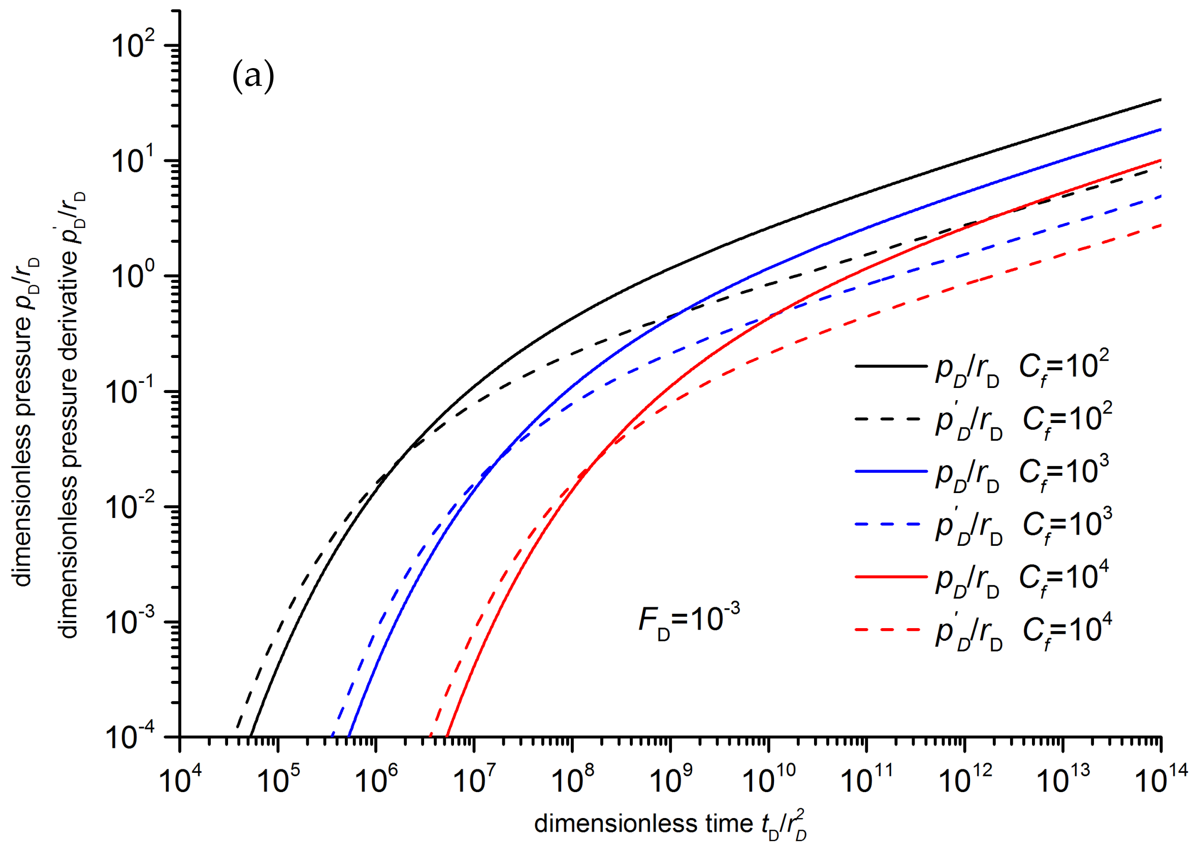
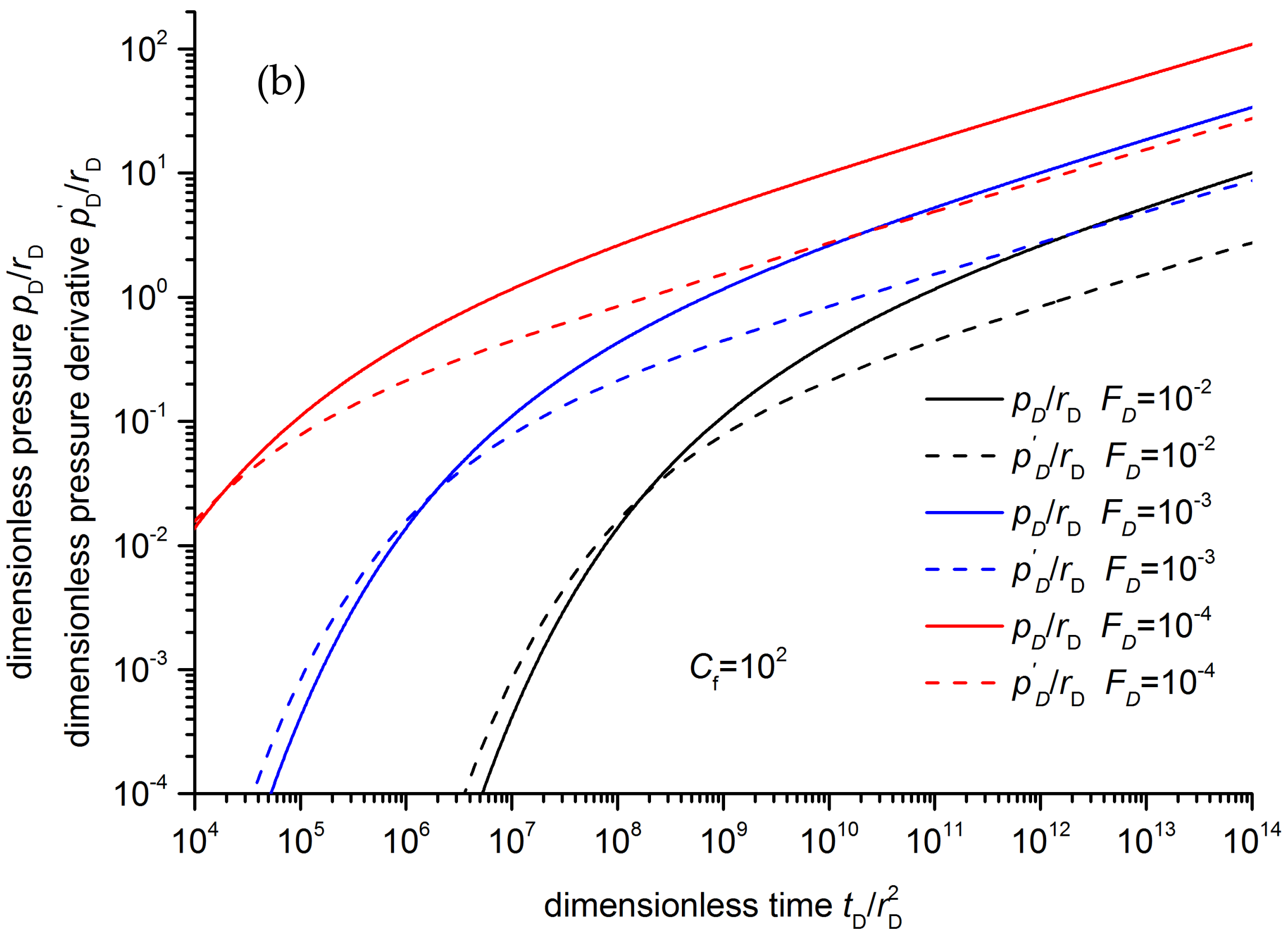
Different connection forms and boundary conditions also reflect their characters in the interference test type-curve. For two wells connected by a homogeneous reservoir, the dimensionless pressure derivative increases and then approaches a 0.5 horizontal line [38]. Therefore, the shapes of their dimensionless pressure derivative curves are highly different. The pressure derivative would appear between the 0.5 horizontal lines and the straight line with a slope of 0.5, when the difference between the conductivity of the large fracture and the matrix is not large enough to ignore the influence of the matrix. Considering the crossflow of the reservoir matrix to the large fracture, the pressure transient can be obtained through Laplace transformation and the Stehfest numerical inversion method. The details can be seen in the Appendix A. The interference test type-curve of WsCLF with a crossflow of reservoir matrix is shown in Figure 5. It can be seen that the pressure and pressure derivative curves approach parallel straight lines with a slope of 0.25. It can be found that FD and Cf have a similar influence on the curves, and they cannot be distinguished. This can also be concluded from Equation (A19).
The intensity of the fractures can affect the shape of the pressure derivative curves. The reservoir approximates a double porosity medium when there are intensive fractures, and the pressure derivative curve has a cavity compared with that of the homogeneous reservoir [41]. The storativity ratio ω is related to the intensity of fractures and can be evaluated by the pressure derivative [38].
Therefore, the appearance of the pressure and pressure derivative curves in the double logarithmic coordinate can be used to diagnose the form of connections. In addition, the fracture intensity can be qualitatively judged based on the deviation of the pressure derivative from that of a homogeneous reservoir and WsCLF.
6. Conclusions
To deal with the situation that there is no practical analysis model of the interference test for WsCLF, an one-dimensional governing equation is established in this study. An analytical solution is further obtained by the similarity transformation method. Using this solution, the extremum equation of the interference test for WsCLF is derived, and the type-curve of the interference test is plotted. Then, interference test data was fitted by the type-curve. It is found that the extremum equation of the interference test for WsCLF differs from that for homogeneous reservoirs by a factor 2. However, it is to be noted that the computed permeability may be quite different because their respective porosity and compressibility are quite different.
On the interference test type-curve of the double logarithmic coordinate, the pressure and pressure derivative curves of WsCLF increase over time, and both finally become straight lines with a slope of 0.5. When the crossflow of the reservoir matrix to the large fracture cannot be ignored, the slope of these straight lines is 0.25. Considering the distinct shapes of pressure derivative curves for different connections, the connection form of wells can be diagnosed and the intensity of fractures can be qualitatively judged through the pressure derivative curves of the interference test.
In this study, it is assumed that the two wells are connected by a large fracture. In fact, when two wells communicate through a narrow, high-permeability strip formation, the flow in the formation is a radial flow near the well and then turns into a linear flow. If the strip is very narrow, the radial flow phase is very short and is even covered by the wellbore storage phase. At this time, the flow characteristics are similar to that of the WsCLF. Therefore, the results of this study can also be used for the analysis of such a situation.
It is difficult to maintain the production rate of gas or oil wells constant in reality. Given that the extremum equation is independent of the production rate, it is only necessary to be able to distinguish the relationship between different active signals. However, when using the type-curve for analysis, the production rate must be considered. If the fluctuation of the production rate is not large over a long time, it can be treated as a constant production period. The average production rate is used in the analysis. Therefore, in order to use the type-curve for analysis, it is necessary to retain a substantially stable production rate over an extended period of time.
Author Contributions
Conceptualization, G.H. and Y.L.; methodology, G.H. and W.L.; formal analysis, G.H. and W.L.; investigation, D.G. and W.L.; writing—original draft preparation, G.H.; writing—review and editing, D.G. and Y.L.; funding acquisition, G.H.
Funding
This research was funded by the National Natural Science Foundation of China, grant number 11602276.
Conflicts of Interest
The authors declare no conflict of interest.
Appendix A. Pressure Transient of WsCLF with Crossflow of the Reservoir
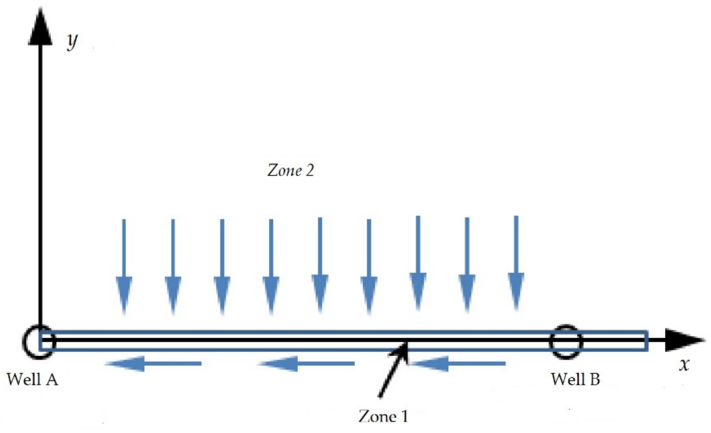
When the crossflow of a reservoir to the large fracture cannot be ignored, the flow regime is shown in Figure A1. Zone 1 is the large fracture, and Zone 2 is the reservoir.
Figure A1.
Flow regime of a large fracture with crossflow of the reservoir.

The dimensionless quantities are defined as follows
where ηm is the pressure conductivity coefficient of reservoir matrix (m2/s), and Km is the permeability of reservoir matrix (m2). It is easy to derive the dimensionless governing equations, initial conditions and boundary conditions. In Zone 1, the governing equation is [42]
The initial conditions and boundary conditions are
In Zone 2, the governing equation is [42]
The initial conditions and boundary conditions are
The followings can be obtained from Equations (A2)–(A9) through Laplace transformation
The following can be derived using Equations (A13) and (A15)
where u is the Laplace transform variable, and c1 is constant with respect to variable yD. By combining Equations (A14) and (A16), it yields
Substituting Equations (A17) and (A16) into Equation (A10) results in
Using Equations (A18), (A11) and (A12), the pressure transient solution of Zone 1 in the Laplace domain can be obtained as follows
The pressure transient solution in the real domain can be obtained using the solution (A19) in the Laplace domain using the Stehfest numerical inversion method.
References
- Kamal, M.M. Interference and pulse test—A review. J. Petrol. Technol. 1983, 35, 2257–2270. [Google Scholar] [CrossRef]
- Estrada, C.A.; Leung, L.; Majcher, M.B.; Johnson, B. Interference test to Characterize the injection behavior of a 20-Acre pattern in the Court Field. J. Can. Pet. Technol. 2008, 47, 31–38. [Google Scholar] [CrossRef]
- Ohaerl, C.U.; Sankaran, S.; Fernandez, J.J. Evaluation of reservoir connectivity and hydrocarbon resource size in a deep water gas field using multi-well interference tests. In Proceedings of the SPE Annual Technical Conference and Exhibition, Amsterdam, The Netherlands, 27–29 October 2014. SPE 170829. [Google Scholar] [CrossRef]
- Kutasov, I.M.; Eppelbaum, L.V.; Kagan, M. Interference well test-variable fluid flow rate. J. Geophys. Eng. 2008, 5, 86–91. [Google Scholar] [CrossRef]
- AI-Harthi, M.A.; Pardo, C.; Kilany, K.; Otaibi, M.A.; Zeybek, M.; Amin, A. Comprehensive reservoir vertical interference test to optimize horizontal well placement strategy in a giant carbonate field. In Proceedings of the SPE Saudi Arabia Section Annual Technical Symposium and Exhibition, Al-Khobar, Saudi Arabia, 21–23 April 2015. SPE 178013. [Google Scholar] [CrossRef]
- Hocking, G. Hydraulic Pulse interference tests for site hydrogeologic characterization. In Proceedings of the 3rd International Conference on Remediation of Chlorinated and Recalcitrant Compounds, Monterey, CA, USA, 20–23 May 2002. [Google Scholar]
- Akin, S. Design and analysis of multi-well interference tests. In Proceedings of the World Geothermal Congress, Melbourne, Australia, 19–25 April 2015. [Google Scholar]
- Theis, C.V. The relation between lowering of the piezometric surface and the rate and duration of discharge of a well using ground-water storage. Transactions AGU 1935, 16, 519–524. [Google Scholar] [CrossRef]
- Ogbe, D.O.; Brigham, W.E. A correlation for interference test with well bore storage and skin effects at both wells. SPE Format. Eval. 1989, 3, 391–396. [Google Scholar] [CrossRef]
- Gringarten, A.C.; Witherspoon, P.A. A method of analyzing pump test data from fractured aquifers. In Proceedings of the Symposium on Percolation through Fissured Rocks, International Society for Rocks Mechanics, Stuttgart, Germany, 18–19 September 1972; Volume 3-B, pp. 1–9. [Google Scholar]
- Chu, L.; Grader, A.S. Transient pressure analysis of three wells in a three-composite reservoir. In Proceedings of the SPE Annual Technical Conference and Exhibition, Dallas, TX, USA, 6–9 October 1991. SPE 22716. [Google Scholar] [CrossRef]
- Onur, M.; Reynolds, A.C. Interference test of a two-layers commingled reservoir. SPE Format. Eval. 1989, 4, 595–603. [Google Scholar] [CrossRef]
- Slack, T.Z. Hydromechanical Interference Slug Tests in a Fractured Biotite Geniss. Master’s Thesis, Clemson University, Clemson, SC, USA, July 2010. [Google Scholar]
- Martinez, N.R.; Samaniego, F.V. Advance in the analysis of pressure interference tests. J. Can. Pet. Technol. 2010, 49, 65–70. [Google Scholar] [CrossRef]
- Malekzadeh, D.; Tiab, D. Interference test of horizontal wells. In Proceedings of the SPE Annual Technical Conference and Exhibition, Dallas, TX, USA, 6–9 October 1991. SPE 22733. [Google Scholar] [CrossRef]
- AI-Khamis, M.; Ozkan, E.; Raghavan, R. Interference test with horizontal observation wells. In Proceedings of the SPE Annual Technical Conference and Exhibition, New Orleans, LA, USA, 30 September–3 October 2001. SPE 71581. [Google Scholar] [CrossRef]
- Awotunde, A.A. Characterization of reservoir parameters using horizontal well interference test. In Proceedings of the SPE Annual Technical Conference and Exhibition, San Antonio, TX, USA, 24–27 September 2006. SPE 106517. [Google Scholar] [CrossRef]
- Sheng, J.J. A new technique to determine horizontal and vertical permeabilities from the time-Delayed response of a vertical interference test. Transport Porous Med. 2009, 77, 507–527. [Google Scholar] [CrossRef]
- Hounli, A.; Tiab, D. Analysis of interference test of horizontal wells in an anisotropic medium. In Proceedings of the SPE Asia Pacific Oil and Gas Conference and Exhibition, Perth, Australia, 18–20 October 2004. SPE 88537. [Google Scholar] [CrossRef]
- Awotunde, A.A.; Ai-Hashim, H.S.; AI-Khamis, M.N.; AI-Yousef, H.Y. Interference test using finite-conductivity horizontal wells of unequal lengths. In Proceedings of the SPE Eastern Regional/AAPG Eastern Section Joint Meeting, Pittsburgh, PA, USA, 11–15 October 2008. SPE 117744. [Google Scholar] [CrossRef]
- Syed, A.F.; AI-Hashim, H.S. Interference test with horizontal wells in layered reservoir. In Proceedings of the Asia Pacific Oil and Gas Conference and Exhibition, Jakarta, Indonesia, 30 October–1 November 2007. SPE 109023. [Google Scholar] [CrossRef]
- Adewole, E.S. Mathematical formulation of interference tests analyses procedure for horizontal and vertical wells both in a laterally infinite layered reservoir. Petrol. Sci. Technol. 2013, 3, 680–690. [Google Scholar] [CrossRef]
- AI-Farhan, F.A.; Gazi, N.H.; AI-Naqi, M.; Ali, F.; Dasti, L.; AI-Qattan, A. Reservoir connectivity analysis using long term interference test in a waterflood pilot in the carbonate Marrat formation of the greater Burgan Field, Kuwait. In Proceedings of the SPE Annual Technical Conference and Exhibition, San Antonio, TX, USA, 8–10 October 2012. SPE 159126. [Google Scholar] [CrossRef]
- AI-Farhan, F.A.; Gazi, N.H.; AI-Humoud, J.; Tirkey, N.; Haryono, R. An interference test coupled with a drawdown analysis of horizontal well using a multi-phase flow meter to evaluate reservoir parameters and connectivity. In Proceedings of the Abu Dhabi International Petroleum Conference and Exhibition, Abu Dhabi, UAE, 11–14 November 2012. SPE 161711. [Google Scholar] [CrossRef]
- Nurafza, P.R.; AI-Shamma, B.; Feng, W.C. Interference test of horizontal producers and injectors in the Huntington. In Proceedings of the International Petroleum Technology Conference, Doha, Qatar, 19–22 January 2014. IPTC 17586. [Google Scholar] [CrossRef]
- Koening, R.A.; Stubbs, P.B. Interference test of a coalbed methane reservoir. In Proceedings of the SPE Unconventional Gas Technology Symposium, Louisville, KY, USA, 18–21 May 1986. SPE 15225. [Google Scholar] [CrossRef]
- Ajani, A.A.; Kelkar, M.G. Interference study in shale Plays. In Proceedings of the SPE Hydraulic Fracturing Technology Conference, The Woodlands, TX, USA, 6–8 February 2012. SPE 151045. [Google Scholar] [CrossRef]
- Kazemi, H.; Seth, M.S.; Thomas, G.W. The interpretation of interference tests in naturally fractured reservoirs with uniform fracture distribution. SPE J. 1969, 9, 463–472. [Google Scholar] [CrossRef]
- Vasilev, I.; Aleksakhin, Y. Interference test in naturally fractured formation gas field case study. In Proceedings of the SPE Russian Petroleum Technology Conference and Exhibition, Moscow, Russia, 24–26 October 2016. SPE 181969. [Google Scholar] [CrossRef]
- Araujo, H.N.; Andina, S.A.; Gilman, J.R.; Kazemi, H. Analysis of interference and pulse tests in heterogenous naturally fractured reservoirs. In Proceedings of the SPE Annual Technical Conference and Exhibition, New Orleans, LA, USA, 27–30 September 1998. SPE 49234. [Google Scholar] [CrossRef]
- Biryukov, D.; Kuchuk, F.J. Transient pressure behavior of reservoirs with discrete conductive faults and fractures. Transport Porous Med. 2012, 95, 239–268. [Google Scholar] [CrossRef]
- Seth, P.; Manchanda, R.; Kumar, A.; Sharma, M. Estimating hydraulic fracture geometry by analyzing the pressure interference between fractured horizontal wells. In Proceedings of the SPE Annual Technical Conference and Exhibition, Dallas, TX, USA, 24–26 September 2018. SPE 191492. [Google Scholar] [CrossRef]
- Weijermars, R.; van Harmelen, A.; Zuo, L.; Alves, I.N.; Yu, W. Flow interference between hydraulic fractures. SPE Reserv. Eval. Eng. 2018, 21, 942–960. [Google Scholar] [CrossRef]
- Morales, A.; Zhang, K.; Gakhar, K.; Porcu, M.M.; Lee, D.; Shan, D.; Malpani, R.; Pope, T.; Sobernheim, D.; Acock, A. Advanced modeling of interwell fracturing interference: An Eagle Ford shale oil study-refracturing. In Proceedings of the SPE Hydraulic Fracturing Technology Conference, The Woodlands, TX, USA, 9–11 February 2016. SPE 179177. [Google Scholar] [CrossRef]
- Chu, W.; Scott, K.; Flumerfelt, R.; Chen, C. A new technique for quantifying pressure interference in fractured horizontal shale wells. In Proceedings of the SPE Annual Technical Conference and Exhibition, Dallas, TX, USA, 24–26 September 2018. SPE 191407. [Google Scholar] [CrossRef]
- Wu, K.; Wu, B.; Yu, W. Mechansim analysis of well interference in unconventional reservoirs: Insights from fracture-geometry simulation between two horizontal wells. SPE Prod. Oper. 2018, 33, 1–9. [Google Scholar] [CrossRef]
- Xiao, C.; Dai, Y.; Tian, L.; Lin, H.; Zhang, Y.; Yang, Y.; Hou, T.; Deng, Y. A semianalytical methodology for pressure-transient analysis of multiwall-pad-production scheme in shale gas reservoirs, part 1: New insights into flow regimes and multiwall interference. SPE J. 2018, 23, 1–21. [Google Scholar] [CrossRef]
- Bourdet, D. Well Test Analysis: The Use of Advanced Interpretation Models; Elsevier Science B.V.: Amsterdam, The Netherlands, 2002; pp. 273–299. [Google Scholar]
- Liu, W.; Yao, J.; Wang, Y. Exact analytical solutions of moving boundary problems of one-dimensional flow in semi-infinite long porous media with threshold pressure gradient. Int. J. Heat. Mass Tran. 2012, 55, 6017–6022. [Google Scholar] [CrossRef]
- Liu, N. Practical Modern Well Test Interpretation Method, 5th ed.; Petroleum Industry Press: Beijing, China, 2008; p. 290. [Google Scholar]
- Deruyck, B.G.; Bourdet, D.P.; Da Prat, G.; Ramey, H.J., Jr. Interpretation of interference tests in reservoirs with double porosity behavior-theory and field examples. In Proceedings of the SPE Annual Technical Conference and Exhibition, New Orleans, LA, USA, 26–29 September 1982. SPE 11025. [Google Scholar] [CrossRef]
- Lee, S.T.; Brockenbrough, J.R. A new approximate analytic solution for finite-conductivity vertical fractures. SPE Forma. Eval. 1986, 1, 75–88. [Google Scholar] [CrossRef]
Figure 1.
Active well production rate and observation well pressure of interference test.

Figure 2.
Schematic diagram of wells connected by a large fracture.

Figure 3.
Interference test type-curve of wells connected by a large fracture.

Figure 4.
Fitting results for interference test data of Chu et al. [36]. (a) 4H well. (b) 6H well.
Figure 4.
Fitting results for interference test data of Chu et al. [36]. (a) 4H well. (b) 6H well.

Figure 5.
Interference test type-curve for wells connected by a large fracture with crossflow of the reservoir. (a) Different Cf. (b) Different FD.
Figure 5.
Interference test type-curve for wells connected by a large fracture with crossflow of the reservoir. (a) Different Cf. (b) Different FD.


© 2019 by the authors. Licensee MDPI, Basel, Switzerland. This article is an open access article distributed under the terms and conditions of the Creative Commons Attribution (CC BY) license (http://creativecommons.org/licenses/by/4.0/).
Share and Cite
MDPI and ACS Style
Han, G.; Liu, Y.; Liu, W.; Gao, D. Investigation on Interference Test for Wells Connected by a Large Fracture. Appl. Sci. 2019, 9, 206. https://0-doi-org.brum.beds.ac.uk/10.3390/app9010206
AMA Style
Han G, Liu Y, Liu W, Gao D. Investigation on Interference Test for Wells Connected by a Large Fracture. Applied Sciences. 2019; 9(1):206. https://0-doi-org.brum.beds.ac.uk/10.3390/app9010206
Chicago/Turabian StyleHan, Guofeng, Yuewu Liu, Wenchao Liu, and Dapeng Gao. 2019. "Investigation on Interference Test for Wells Connected by a Large Fracture" Applied Sciences 9, no. 1: 206. https://0-doi-org.brum.beds.ac.uk/10.3390/app9010206
Note that from the first issue of 2016, this journal uses article numbers instead of page numbers. See further details here.