Characteristic Analysis and Experiment of Adaptive Fiber Optic Current Sensor Technology

School of Electrical and Electronic Engineering, North China Electric Power University, Beijing 102206, China
*
Author to whom correspondence should be addressed.
Appl. Sci. 2019, 9(2), 333; https://0-doi-org.brum.beds.ac.uk/10.3390/app9020333
Submission received: 27 December 2018
/
Revised: 14 January 2019
/
Accepted: 16 January 2019
/
Published: 18 January 2019
(This article belongs to the Special Issue Recent Progress in Fiber Optic Sensors: Bringing Light to Measurement)
Abstract
:The straight-through magneto-optical glass current sensor has desirable temperature properties, but it is vulnerable to magnetic interference. In contrast, a polarization-type fiber optic current sensor has poor temperature performance, but the magnetic anti-interference characteristic is very good. Aiming at the problem that the accuracy of a fiber optic current sensor is susceptible to external disturbances and temperature fluctuations, we present an adaptive technology of a fiber optic current sensor that uses the magneto-optical output signal to correct the fiber output signal. The working principle of the improved method is introduced in this paper. The structure of the specific optical system and the signal processing system are presented. Temperature fluctuation and magnetic change detection units are included in the design in order to provide signal selection under different environmental fluctuations, thus stabilizing the output current data. The signal processing system was proved to be effective by building an experimental platform.
1. Introduction
With the development of the smart grid, sensors in electric power systems have stricter requirements. Compared with a traditional electromagnetic current sensor, a fiber optic current sensor has outstanding advantages such as excellent insulation performance, lack of magnetic saturation without ferromagnetic resonance, a wide frequency response range, and good dynamic performance [1,2]. It has potential application in metering protection, real-time data monitoring, and fault diagnosis analysis in power systems [3,4].
The sensing fiber in a fiber optic current sensor is a closed circle structure with good magnetic field characteristics [5], but the fiber is sensitive to temperature changes. When the temperature fluctuates between −10 °C and 60 °C, the experimental ratio error varies from −0.648% to 0.673%. A greater temperature fluctuation exacerbates the fiber optic current sensor error drift [6]. Thus, temperature fluctuations degrade the accuracy of the system, which has become a major limit in its practical application [7]. Many scholars have carried out related research. The influence of ambient temperature on a quarter wave plate and Verdet constant were analyzed in a prior study, and the resulting fiber optic current sensor error expression was derived [8]. Variable temperature parameters and a fiber optic current sensor-equivalent digital control model were introduced, and the influence of temperature on steady-state output accuracy from a fiber optic current sensor was simulated [9].
Some publications proposed measures for compensating temperature drift based on an analysis of the influence of temperature on fiber optic current sensor accuracy. Compensation of Verdet constant temperature dependence by crystal core temperature measures the temperature of the same volume of crystal that affects the beam polarization in a magnetic field or current sensing process [10]. A suitable initial phase delay angle can be selected to compensate changes in the Verdet constant caused by temperature when constructing a quarter-wave plate [11]. A polynomial model for describing errors due to temperature fluctuations was also established [12]. Least squares regression was used to determine the polynomial coefficients from experimental data gathered at different temperatures, and errors were dynamically compensated based on the actual temperature. A temperature sensor was also used to measure external temperature changes, and a corresponding algorithm was used to compensate the actual error caused by temperature fluctuations [13]. However, compensation requires accurate temperature measurements of the fiber optic current sensor itself rather than the external ambient temperature, making real-time measurement difficult. It is also impossible to establish a mathematical model relating accurate temperature compensation and output error. The model is complex and the coefficient is difficult to determine, thus the method of applying compensation based on changes in ambient temperature is not feasible.
The state of art of fiber optic current sensor typically employs Sagnac interference sensors, reflective sensors or polarization-type fiber optic sensor. A detailed review of all-fiber sensors and bulk-optic current sensor [14] stated that the fiber is vulnerable to temperature gradients, and the high Verdet constants in magneto-optic glass allows for sensors with high sensitivities. In order to solve the polarization-type fiber optic current sensor measurement accuracy problem caused by temperature changes, we propose using a magneto-optical glass sensing signal to correct the fiber output signal. An adaptive method of fiber optic current sensor is designed, which provides a new method for solving the temperature drift problem and providing stable operation in a power system.
2. Open Loop Mechanism of Polarization-Type Fiber Optic Current Sensor
Figure 1 shows the polarization-type fiber optic current sensor. The fiber optic current sensor can be divided into three parts: a light source, a sensing system, and a photoelectric conversion system.
During light propagation in the absence of birefringence, refractive index , , incident linearly polarized light waves can be decomposed into left and right circularly polarized light corresponding to the different propagation coefficients and :
where χ is the polarizability tensor of the medium , c is the speed of light in the vacuum, and ω is the optical frequency.
After light passes through an ideal fiber of length dl, the rotation angle of the electric vector is
In the presence of birefringence, , refractive index , the propagation coefficients are:
After light passes through an ideal fiber of length dl, the rotation angle of the electric vector is:
The photoelectric conversion system converts the light signal into an electric signal. Then the electrical signal is input to a computer system through an interface for post-processing, so as to obtain the magnitude of the measured current. A PIN photodetector is often used. The signal output from the photodetector can be expressed as:
where IP is the output current, JP is the luminous flux, VP is the voltage across the photoelectric converter, hf is the sensitivity of photodetector, and h0 is the conductance parameters of the photodetector.
The output signal from the signal processing circuit is:
where Uout is the output signal from the signal processing circuit, Js and Jp are the output signals of the two linearly polarized beams passing through the photodetector, respectively, and Jsave and Jpave are the DC components corresponding to the two optical paths, respectively.
The influence of external factors like temperature drift on the fiber optic current sensor can be equivalently converted into an additional magnetic field. The temperature-dependent magnetic field can be written as follows:
where Hν is the temperature-dependent equivalent magnetic field, H is the magnetic field induced by the measured current, ν is a coefficient related to the molecular field, C is the Curie constant, and TP is the paramagnetic Curie temperature.
The open loop system diagram of a polarization-type fiber optic current sensor can be derived from this model, as shown in Figure 2.
One can see from Figure 2 that the input variables I1 and T have only positive feedback, thus the fiber optic current sensor is an open loop system [15].
In fact, the difference between the refractive indices of the core and cladding is much less than 1% in a general sensing fiber. After invoking weak derivatives approximation, light transmission in the fiber optic current sensor is the same as in a magneto-optical glass current sensor. Both of the sensors are open loop systems, i.e. the measurement accuracy is determined by the environment and the open loop mechanism. Therefore, an external closed loop is required if stable output is desired from a fiber optic current sensor.
3. Impact of Temperature Drift on a Fiber Optic Current Sensor
Temperature drift has a long duration but slow rate of change, where the duration is measured in seconds. Transient mutation of the magnetic field is fast and may be caused by external overvoltage interference, where the duration is measured in microseconds.
A fiber optic current sensor has a closed circle structure, which satisfies Ampère’s circuital law. After integration, the derived current is similar to the current being measured, so the transient magnetic field mutation produces a weak effect:
Temperature drift lasts for a long time. A fiber optic current sensor is wound with a multi-turn coil, so the optical path is long. The temperature change produces strong interference in the fiber optic current sensor, and the temperature disturbance generates birefringence in the optical fiber, thus changing the rotation angle.
Faraday’s effect and Ampère’s circuital law can be used to derive the rotation angle in the sensing as:
where N is the number of winding turns in the sensing fiber, V is the Verdet constant of the optical fiber, and i is the measured current.
A multi-turn optical fiber forms a closed light path, so the fiber signal is shielded from external magnetic field interference. However, the fiber is sensitive to temperature fluctuations, producing changes in the Verdet constant [16]:
where ΔT = T − T0, T is the actual temperature, T0 = 25 °C, and V0 = 1.0 × 10⁻⁶ rad/A at 25 °C.
On the other hand, the installation of a sensing ring inevitably causes the fiber to bend, and temperature fluctuations generate a stress difference along the cross section of the curved fiber, thereby generating stress-induced birefringence. Q is the temperature-induced linear birefringence coefficient per unit length [17]:
where λ is the wavelength of light, ν is Poisson’s ratio, p12 and p11 are components of the photoelastic tensor, A is the fiber radius, R is the fiber bending radius, and α is the fiber thermal expansion coefficient.
When temperature drift occurs, the actual rotation angle is:
where δ0 is the residual linear birefringence per unit length, and l is the fiber length.
3.1. Comsol Simulation Models
3.1.1. Geometric Model
We adopted wave optics and a magnetic field module in simulation. When using wave optics to analyze the optical field characteristics, the length of sensing units should be close to the wavelength 1310 nm, so usually in the micron scale. The three-dimensional equivalent model of optical sensing units is shown in Figure 3. The cylinder with a smaller radius is used as a model of the conductor. The optical fiber was selected as the sensing unit in a COMSOL simulation and the micro-arc is built to simulate a bending fiber. Its bending radius is 15 cm, the central angle is 4.87° and the fiber core radius is 9 µm. The cylinder with the larger radius is with the air region as the simulation domain to solve magnetic fields.
3.1.2. Material Selection
The material, relative dielectric constant εr, relative magnetic permeability µr, and refractive index n in each simulation region are shown in Table 1.
When the current was set to 2 kA, the Verdet constant increases linearly with temperature at 0.7 × 10⁻⁴ rad/(A∙℃), δ0 = 0, and Q = 5.89 × 10⁻³ rad/°C. Temperature fluctuations were set to ∆T to 0 ℃, 20 °C, and 40 °C. The relationships between the rotation angle θ and the transmission distance L for different temperature changes are shown in Figure 4, and the maximum rotation angle θmax and the corresponding angle error ∆θ are shown in Table 2.
One can infer from Figure 4 that the rotation angle is almost linear with transmission distance when ∆T = 0 °C. When ∆T ≠ 0 °C, θ is no longer linear with L as the transmission distance increasing, the curve becomes nonlinear and also the maximum rotation angle reduces. This is due to the cumulative effects of temperature drift with increased transmission distance because the fiber signal is multiplied by a coefficient that is less than 1. The greater the temperature fluctuation, the larger is the deviation of the rotation angle. According to Table 2, a greater temperature fluctuation results in greater deviation in the rotation angle, which is consistent with Equation (12).
4. Effect of Magnetic Field Changes on a Straight-Through Magneto-Optical Glass Current Sensor
A straight-through magneto-optical glass current sensor can solve the temperature drift problem due to the use of diamagnetic material. If a diamagnetic material is selected, it is no longer necessary to consider the influence of temperature on the Verdet constant, resulting in stable temperature performance. This kind of current sensor has a small volume and a short optical path, and it is difficult to satisfy the closed loop integral in Ampère’s circuital law. Therefore, a sudden non-uniform magnetic field will create interference in a magneto-optical glass current sensor.
Faraday’s effect and the Biot-Savart law can be used to derive the rotation angle through magneto-optic glass:
where VG is the Verdet constant of the magneto-optical glass, L is the length of magneto-optical glass, and h is the distance between the current wire and magneto-optical glass.
Magneto-optical glass is in an open optical circuit, in contrast with the closed circle structure of the sensing fiber. The magneto-optical signal is affected by internal magnetic field changes caused by current changes and external magnetic field interference. When the internal or external magnetic field changes, the rotation angle will change to:
where ΔH is the magnetic field changes.
4.1. Comsol Simulation Models
4.1.1. Geometric Model
Magneto-optical glass was selected as the sensing unit in a COMSOL simulation. The geometric model of magneto-optic glass is a rectangle with a height and width of 2 µm and a length of 10µm. In the COMSOL simulation, the size of magneto-optical glass is set in micrometers in order to better observe the light propagation process. The cylinder with the larger radius is with the air region as the simulation domain to solve magnetic fields. The three-dimensional equivalent model of magneto-optical glass sensing units is shown in Figure 5.
4.1.2. Material Selection
The material, relative dielectric constant εr, relative magnetic permeability µr, and refractive index n in each simulation region are shown in Table 3.
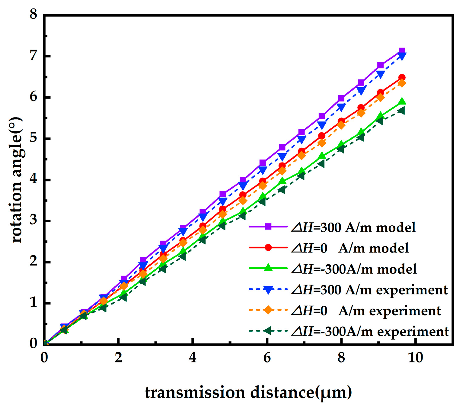
The current was set to 2 kA, and the magnetic field change ∆H was set to 0 A/m, –300 A/m, 300 A/m. The relationship between the rotation angle θ and the transmission distance L for different magnetic field changes is shown in Figure 6, and the maximum rotation angle θmax and the corresponding angle error ∆θ are shown in Table 4.
Figure 6 and Table 4 show that the rotation angle increases linearly with transmission distance. A greater change in magnetic field and longer distance lead to larger deviations in rotation angle. ∆θ = −0.0106 rad ≈ V∆HL when ∆H = −300 A/m, and ∆θ = 0.0110 rad ≈ V∆HL when ∆H = 300 A/m. It can be seen that the magneto-optical output signal is superimposed with an offset linearly related to the distance when the magnetic field changes, which is consistent with Equation (14).
The above analysis shows that the optical fiber output signal is sensitive to temperature drift, while magneto-optical glass is sensitive to magnetic field changes. Therefore, an adaptive technology of fiber optic current sensor is required in order to achieve stable output from the sensor under temperature fluctuations.
5. Adaptive Technology of Fiber Optic Current Sensor
An independent variable must be added in order to imbue the fiber optic current sensor with adaptive characteristics. A new independent variable that is related to the output signal is introduced externally. The system has a feed forward characteristic that yields the output signal independent of temperature interference, thus improving measurement accuracy.
A schematic diagram of the adaptive fiber optic current sensor is shown in Figure 7, where the box with south-east arrow indicates adjustable characteristics. Compensating adjustment in the relevant parameters is performed with an adaptive algorithm that is driven by the output of the fiber optic current sensor, and the signal analysis.
The sensor unit in the adaptive fiber optic current sensor adds two magneto-optical glasses. The optical system part outputs three signals and includes temperature fluctuation detection and magnetic change detection in real-time signal processing systems. The average value of the fiber signal and the magneto-optical glass signal are the output during stable operation. The magneto-optical signal is used for correction when the temperature fluctuation causes the optical fiber output to fluctuate. When there is a sudden change in the external magnetic field, the output of fiber optic current sensor is maintained.
The design allows selection of the output signal under different conditions, which suppresses magnetic interference in the closed optical fiber sensing ring and overcomes the output fluctuation problem caused by temperature drift.
5.1. Optical System Structure
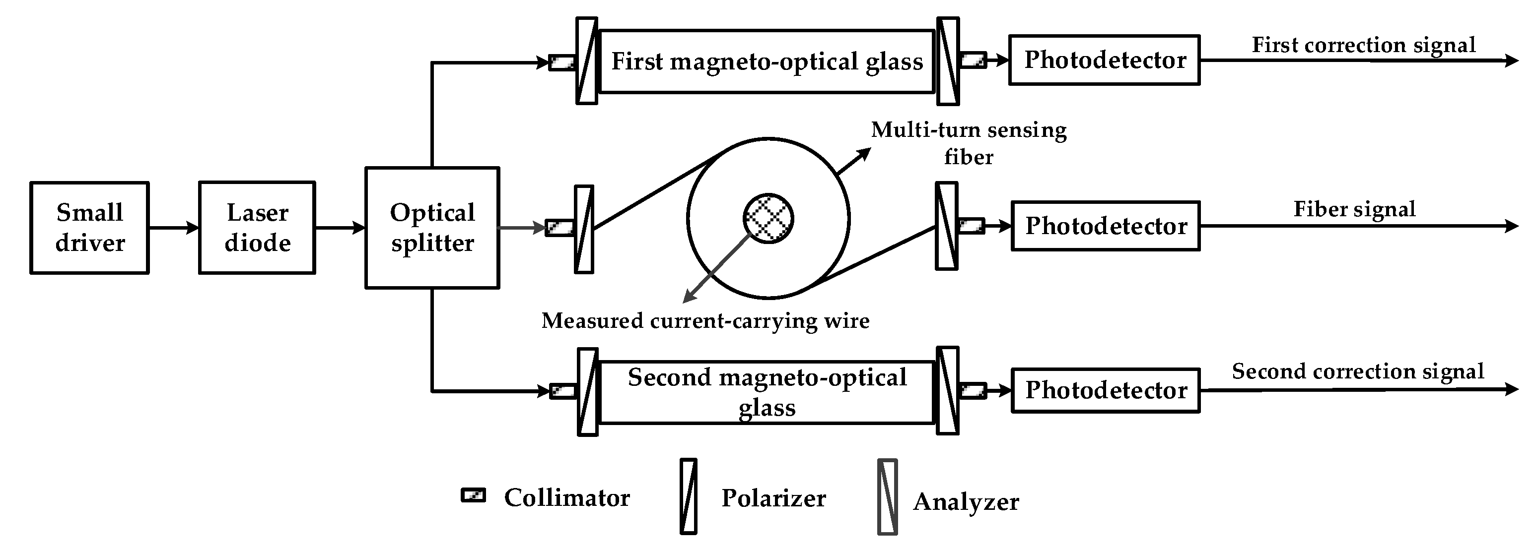
The adaptive method is based on the polarization-type fiber optic current sensor. Magneto-optical glasses are added on both sides of the optical fiber [18]. The specific structure of the optical system is shown in Figure 8. A small driver works at a constant current or constant power mode to drive a laser diode to output linearly polarization light. The incident light is split into three beams with factors K1, K2, and (1 – K1– K2) with an optical splitter, where 0.001 < K1 < 0.999, 0.001< K2 < 0.999, and 0.001 < K1 + K2 < 0.999. Each beam of light passes through a collimator, polarizer, sensing material, analyzer, and collimator. Finally, the light signal is converted to an electrical signal with a photodetector for further signal selection and processing.
The fiber signal uF can be expressed as follows:
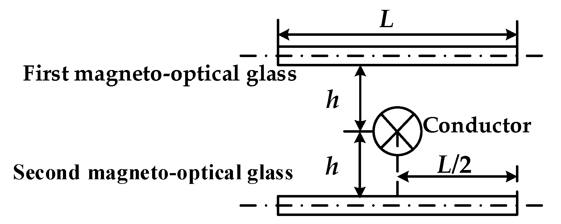
Two pieces of magneto-optical glass with the same size and material are used as sensing units for signal correction. They are placed symmetrically on both sides of the conductor. The arrangement is shown in Figure 9.
The first and second correction signal can be expressed as follows:
where P0 is the power of the light source, K is the factor, θ is the Faraday rotation angle.
5.2. Real-Time Signal Processing System
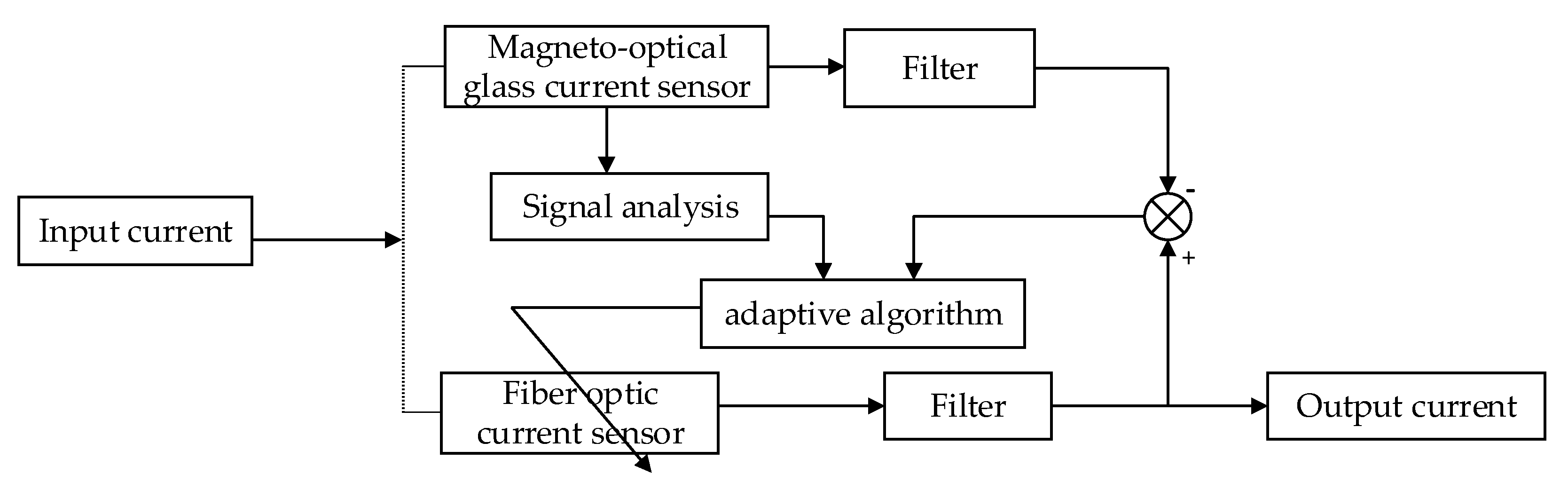
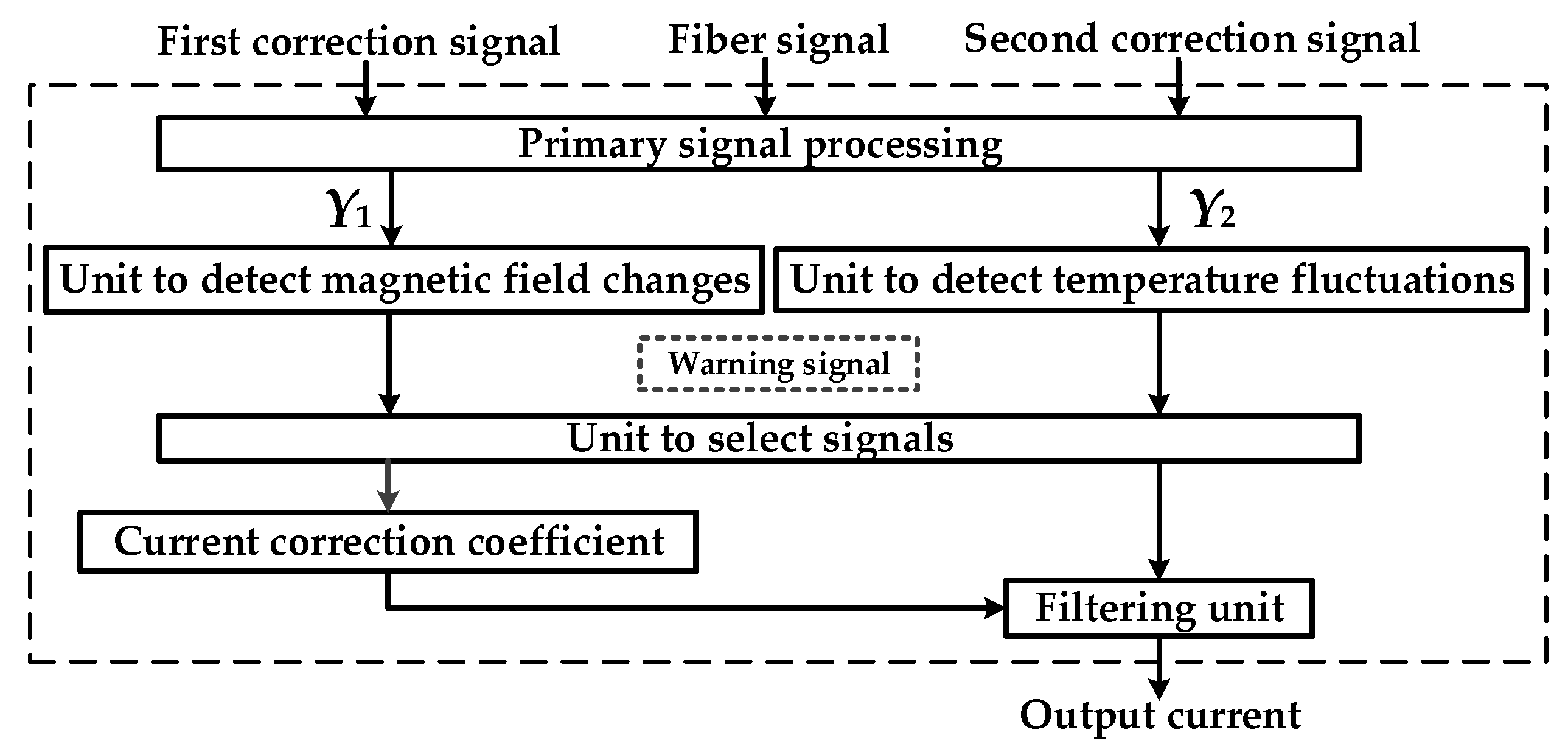
The output signal is processed to obtain the magneto-optical correction signal Y1 and a fiber optic AC signal Y2. Then Y1 enters the magnetic change detecting unit, and Y2 enters the temperature fluctuation detecting unit. The detecting unit outputs a warning signal to the signal selection unit, which subsequently determines the proportionality coefficient for signal correction, and a current is output through the filtering unit. The structure of the real-time signal processing system is shown in Figure 10.
(1) Primary signal processing
The coefficient adjustment make correction signal 1 and correction signal 2 be equal. The two signals are subtracted to obtain a magneto-optical compensatory correction signal:
Substituting Equations (15) and (16) into Equation (17):
according to Equation (13), where
The magneto-optical compensatory correction signal Y1 obtained from the primary signal processing unit does not include a DC component and is proportional to the measured current. Signal subtraction will weaken the external interference effect when there is a certain degree of external magnetic interference, thus two magneto-optical glasses are used for compensation. The rotation angles along the directions of the two beams are opposite, thus the magnetic field change caused by current changes will double after subtraction.
The correction coefficient between the fiber signal and the magneto-optical signal is defined as follows:
Substituting the corresponding output signal yields an AC optical fiber signal:
where
The AC optical fiber signal Y2 does not contain a DC component. Y2 is only proportional to the measured current after the light source and the sensing fiber parameters are determined.
(2) Detecting magnetic field changes
Magnetic field changes are calculated using the compensatory correction signal Y1 obtained from the primary signal processing unit:
where Y1m is the m′th peak AC value in Y1.
The magnetic change warning value is defined as SetB. P1m > SetB indicates that the magnetic field has changed, and the detection unit outputs WB = 1. The measured current will contain waveform distortion when the power system changes from the steady state to the transient state and the signal analysis method can be used to detect the moment of mutation. By observing whether waveforms Y1 and Y2 are equivalent, one can determine whether the change is caused by external magnetic field interference or the input current itself. If waveform distortion is present in both, then the change is caused by the measured current. If only Y1 is distorted and Y2 is unchanged, the magnetic field change is due to external magnetic interference. At this time, the compensatory correction signal is locked in order to maintain the fiber optic current sensor output. WB = 0 when P1m ≤ SetB.
(3) Detecting temperature fluctuations
Temperature fluctuations are calculated using the fiber optic current sensor output signal Y2:
where Y2m is the m′th peak AC value in Y2.
The temperature fluctuation warning value SetT is set in order to output a corresponding warning signal in the presence of temperature fluctuations. P2m > SetT indicates that the temperature has changed, and the detection unit outputs WT = 1. WT = 0 when P2m ≤ SetT.
(4) Signal selection unit
The sensor operates stably when WB = 0 and WT = 0, and the average fiber optic current sensor signal value and the magneto-optical signal are selected as the output value. Here one can define Y = (Y1 + Y2)/2 and the proportionality coefficient is set to M = (M1 + M2)/2. The filtered output AC signal is accurately converted to the input current signal.
The magnetic field is stable when WB = 0 and WT = 1, and the output from the fiber optic current sensor fluctuates due to temperature drift. Thus, the magneto-optical signal corrects the fiber signal, setting the proportionality coefficient to M = M1, which is subsequently input to the filtering unit.
There is a transient magnetic field when WB = 1 and WT = 0, and the fiber optic current sensor output value will not be corrected by the magneto-optical glass output signal. The fiber AC output is stable, the fiber AC signal Y2 is selected as the final output signal, and the current proportionality coefficient is set to M = M2.
(5) Filtering unit
The filtering unit filters the output from the signal selecting unit, the noise in the current sensor is mainly white noise [19], and the output signal is filtered using linear Kalman filtering. The specific steps are as follows:
where Ak−1 and I are third order unit arrays, Xk = [x1,x2,x3]T, Xk−1 is the state variable before each cycle, Xk|k−1 is the preliminary prediction of the state variable, Xk is the state variable after each cycle, Pk−1 is covariance matrix before update, Pk|k−1 is the preliminary prediction covariance matrix, Pk is the covariance matrix after the update, Yk is the sampling measurement that is input by the signal selecting unit, Kk is Kalman filter gain matrix, H = [sin(100πt),cos(100πt),1], Q and R are the first covariance and the second covariance, respectively, and the range of values is from 0 to 1.
The filtered AC signal output is:
The output current signal is obtained by setting the proportionality coefficient M from the signal selection unit:
where i is the real-time AC current value and φ is the current phase angle.
6. Experiment
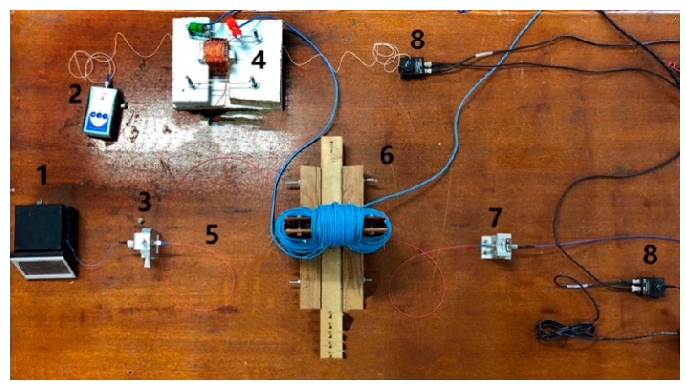
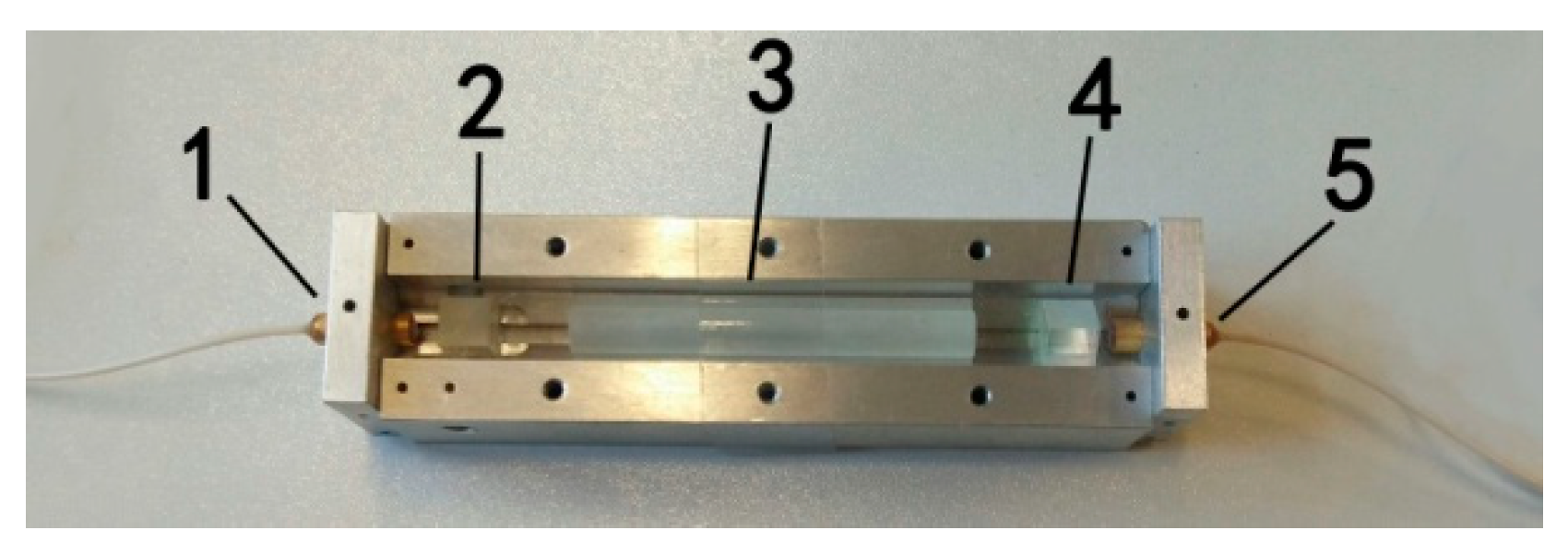
In the experiment, the two optical paths pass through the magneto-optical glass and the optical fiber respectively as Figure 11 shows, then enter the labview signal processing system through the photodetector. The light source of fiber optic current sensor is an LPS-PM1310-FC (THORLABS, Shanghai, China) 1310 nm laser diode with an extinction ratio of 28.2 dB driven by a compact laser diode controller. The wavelength of magneto-optic current sensor’s light source is 850 nm. The sensing fiber is made of low-birefringence fiber (Spun LoBi Fiber). The MR-1 magneto-optical glass in the solenoid structure is diamagnetic, which is independent of temperature with higher sensitivity and stability. The diameter of magneto-optical glass is 4.5 mm, the length of it is 40 mm as Figure 12 shows.
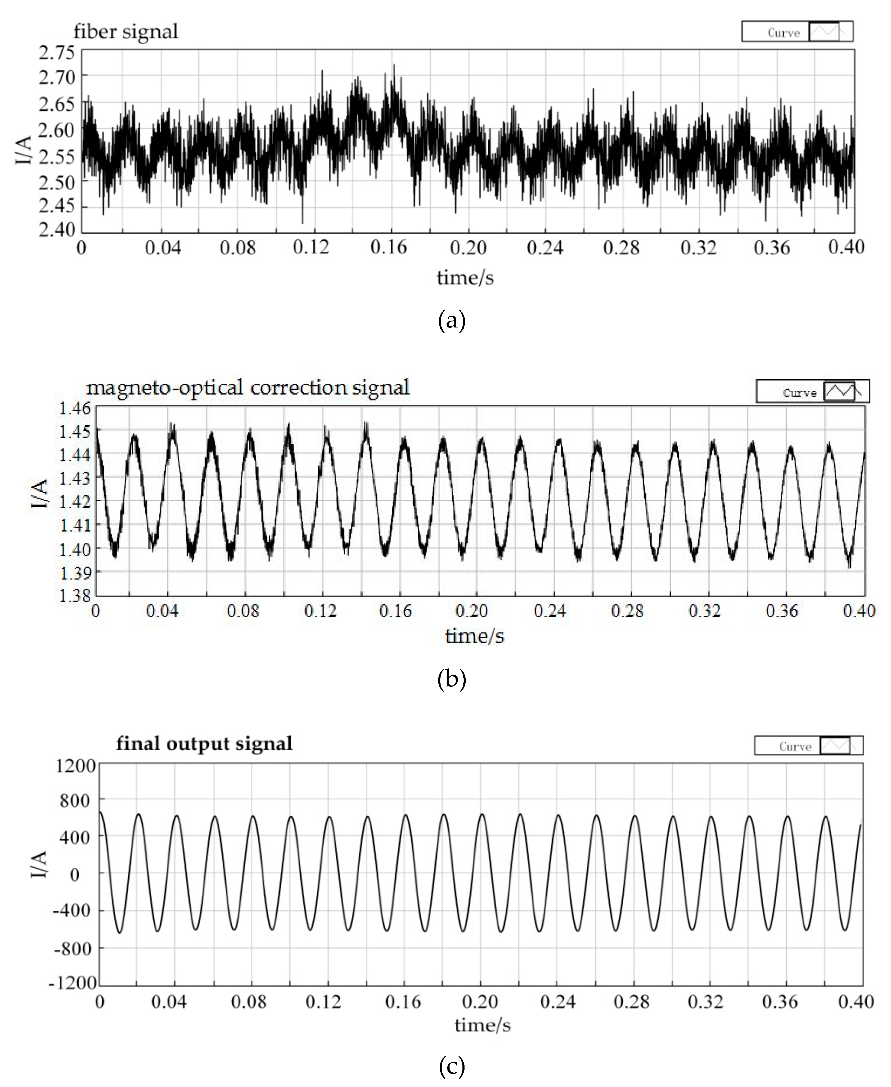
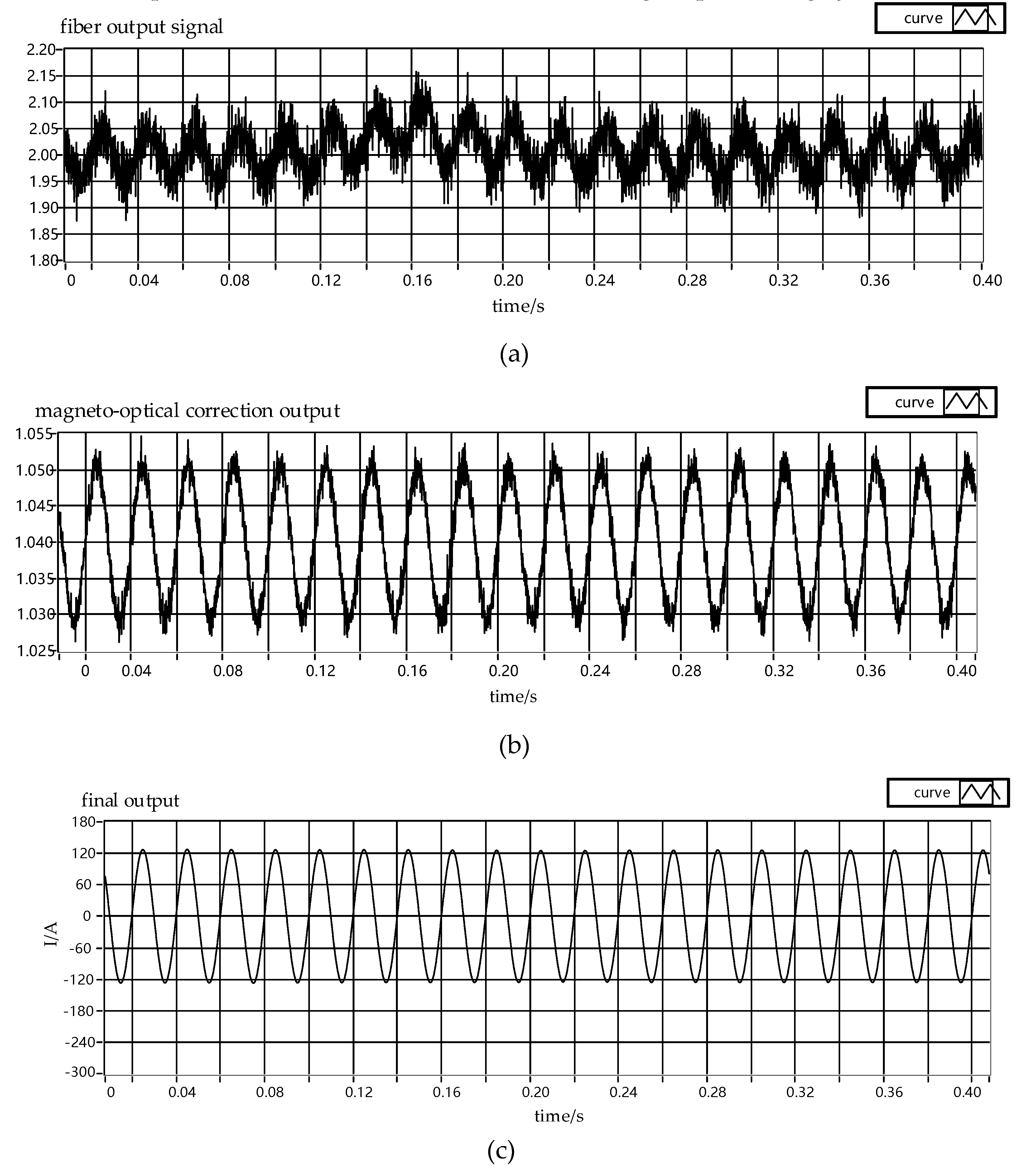
In the experiment, 1.5 A AC is energized by Agilent AC power, the frequency of alternative current is 50 Hz, the number of turns of the coil was 300, and the equivalent current was 450 A. The fiber signal is disturbed by temperature drifts, and the signal fluctuates as Figure 13a shows, but the output signal of the magneto-optical glass is still a stable sine wave as Figure 13b shows, and the final signal output as Figure 13c shows is obtained after processing by Labview. The final current output RMS value obtained after signal processing is 448.8 A, the accuracy of the adaptive method is 0.267%.
When decreasing the input current to 0.3 A AC which is equivalent to RMS 90 A, the result shows the output RMS value is 89.74 A, the accuracy of it is 0.289%. Figure 14 shows the result of the test of 0.3 A. The experiment verifies the effectiveness of the signal processing system.
7. Conclusions
The open loop structure of the polarization-type fiber optic current sensor is the fundamental reason for the low accuracy of fiber optic current sensor measurements. In this paper, an external closed loop system was formed by introducing magneto-optical glasses for signal correction.
We propose an adaptive technology of a fiber optic current sensor that takes advantage of the good anti-magnetic interference ability of a fiber optic current sensor and the desirable temperature stability of a magneto-optical glass current sensor. We verify the effectiveness of the Labview signal processing system by setting up an experimental platform. The combination of the two systems is passive, providing desirable insulation performance. The steady and transient state accuracy of the current sensor are effectively improved, thus eliminating the influence of temperature drift on the fiber optic current sensor measurements.
The adaptive fiber optic current sensor additionally has two output channels, which is also a redundant design for power system protection. Compared with the use of a separate optical current sensor, it is more resistant to interference and provides more accurate measurements.
Author Contributions
Conceptualization, Y.S.L.; writing—original draft preparation, writing—review and editing, W.W.Z.; software, X.Y.L.; formal analysis J.L.
Funding
This research received no external funding.
Conflicts of Interest
The authors declare no conflict of interest.
References
- Li, C.; Lin, H.; Xu, Q.F. New design of OCT with Faraday rotation angle linear measurement. Trans. China Electrotech. Soc. 2015, 32, 46–54. [Google Scholar]
- Qi, X.W.; Yin, X.G.; Li, G.; Zhang, Z.; Wang, Y. A construction method for the simulation platform for the analysis of the current transformer. Power Syst. Prot. Control 2015, 43, 69–76. [Google Scholar]
- Ma, Z.W.; Xie, J. Brief introduction of common current transformer in Substation. Electr. Eng. 2017, 1, 133–136. [Google Scholar]
- Li, Y.S. Theory, Method and Application of Optical Current Transformer; Science Press: Beijing, China, 2015. [Google Scholar]
- Chen, S.; Guo, Z.Z.; Zhang, G.Q.; Yu, W.B.; Yan, S. Distributed parameter model for characterizing magnetic crosstalk in a fiber optic current sensor. Appl. Opt. 2015, 54, 10009–10017. [Google Scholar] [CrossRef] [PubMed]
- Li, Y.S.; Liu, X.Y.; Zhang, W.W.; Liu, J. Error characteristic analysis and experimental research on a fiber optic current transformer. Appl. Opt. 2018, 57, 8359–8365. [Google Scholar] [CrossRef] [PubMed]
- Song, X.K.; Yan, P.L.; Xiao, Z.H.; Liu, D.W.; Li, Y.B. Comment on the technology and application of fiber optic current transformer. Power Syst. Protect. Control 2016, 44, 149–154. [Google Scholar]
- Yin, S.Y.; Zhang, S.C.; Wu, T. Temperature error analysis and temperature error compensation of the all fiber optic current transformer. Electr. Meas. Instrum. 2017, 54, 16–21. [Google Scholar]
- Qing, L.; Daiyin, F.; Peng, M.; Ning, Y. Real-time dynamic simulation model of fiber optical current transformer considering temperature characteristics. Power Syst. Technol. 2015, 39, 1759–1764. [Google Scholar]
- Petricevic, S.J.; Mihailovic, P.M. Compensation of Verdet Constant Temperature Dependence by Crystal Core Temperature Measurement. Sensors 2016, 16, 1627. [Google Scholar] [CrossRef] [PubMed]
- Xiao, H.; Liu, B.Y.; Wan, S.W.; Zhao, Y.C. Temperature error compensation technology of all-fiber optical current transformers. Autom. Electr. Power Syst. 2011, 35, 91–95. [Google Scholar]
- Li, Y.Y.; Yang, X.J.; Xu, J.T.; Wang, Y.L. Temperature Compensation in Full Optical Fiber Current Transformer using Signal Processing. In Proceedings of the 6th International Symposium on Computational Intelligence and Design, Hangzhou, China, 28–29 October 2013; pp. 227–230. [Google Scholar]
- Cheng, S.; Guo, Z.Z.; Zhang, G.Q.; Shen, Y.; Song, P.; Huang, H.W. Temperature characteristic of fiber optic current sensor. High Volt. Eng. 2015, 41, 3843–3848. [Google Scholar]
- Silva, R.M.; Martins, H.; Nascimento, I.; Baptista, J.M.; Ribeiro, A.L.; Santos, J.L.; Jorge, P.; Frazão, O. Optical Current Sensors for High Power Systems: A Review. Appl. Sci. 2012, 2, 602–628. [Google Scholar] [CrossRef] [Green Version]
- Li, Y.S.; Li, X.; Liu, J. Mechanism analysis and modeling on the sensing of fiber-optical current transformer. Proc. CSEE 2016, 36, 6560–6569, 6624. [Google Scholar]
- Williams, P.A.; Rose, A.H.; Day, G.W.; Milner, T.E.; Deeter, M.N. Temperature dependence of the Verdet constant in several diamagnetic glasses. Appl. Opt. 1991, 30, 1176–1178. [Google Scholar] [CrossRef] [PubMed]
- Li, Y.S.; Wang, B.; Liu, J. Modeling analysis and experiment study on temperature characteristic of all-fiber optical current transformer. Proc. CSEE 2018, 38, 2772–2782, 2847. [Google Scholar]
- Bucholtz, F.; Koo, K.P.; Dandridge, A. Effect of external perturbations on fiber-optic magnetic sensors. J. Lightwave Technol. 1988, 6, 507–512. [Google Scholar] [CrossRef]
- Kumai, T.; Nakabayashi, H.; Hirata, Y.; Takahashi, M.; Terai, K.; Ihniuisbi, T.; Uebar, K. Field trial of optical current transformer using optical fiber as Faraday sensor. In Proceedings of the Power Engineering Society Summer Meeting, Chicago, IL, USA, 21–25 July 2002; pp. 920–925. [Google Scholar]
Figure 1.
Structure of the polarization-type fiber optic current sensor.

Figure 2.
Open loop in a polarization-type fiber optic current sensor.

Figure 3.
Geometric model of optical fiber units.

Figure 4.
Effects of the temperature fluctuations on the relationships between θ and L in the optical fiber.
Figure 4.
Effects of the temperature fluctuations on the relationships between θ and L in the optical fiber.

Figure 5.
Geometric model of magneto-optical glass units.

Figure 6.
Effects of magnetic field changes on the relationship between θ and L.

Figure 7.
Schematic diagram of the adaptive fiber optic current sensor.

Figure 8.
Optical system of the adaptive fiber optic current sensor.

Figure 9.
Position of the measured current and two pieces of magneto-optical glass.

Figure 10.
Real-time signal processing system in the adaptive fiber optic current sensor.

Figure 11.
Experimental platform: 1. Compact laser diode controller and laser diode; 2. Light source; 3. Polarizer; 4. Magneto-optical glass sensor; 5. Sensing optical fiber (Between two splints); 6. Input alternative current; 7. Analyzer; 8. Photodetector.
Figure 11.
Experimental platform: 1. Compact laser diode controller and laser diode; 2. Light source; 3. Polarizer; 4. Magneto-optical glass sensor; 5. Sensing optical fiber (Between two splints); 6. Input alternative current; 7. Analyzer; 8. Photodetector.

Figure 12.
Magneto-optical glass sensor: 1. Collimator; 2. Polarizer; 3. Magneto-optical glass; 4. Analyzer; 5. Collimator.
Figure 12.
Magneto-optical glass sensor: 1. Collimator; 2. Polarizer; 3. Magneto-optical glass; 4. Analyzer; 5. Collimator.

Figure 13.
(a) fiber signal; (b) magneto-optical glass signal; (c) final output signal.

Figure 14.
(a)fiber signal; (b) magneto-optical glass signal; (c) final output signal.


Table 1.
Material Parameters.
| Region | Material | εr | µr | n |
|---|---|---|---|---|
| Wire | Copper | 1 | 0.9999 | -- |
| Air region | Air | 1 | 1 | 1 |
| Sensing fiber | SiO2 | 2.09 | 1 | 1.45 |
Table 2.
Maximum rotation angle θmax and angle error ∆θ for different temperature changes.
| Temperature Fluctuation ∆T (°C) | 0 | 20 | 40 |
|---|---|---|---|
| θmax (°) | 6.482 | 5.979 | 5.502 |
| ∆θ (°) | 0 | −0.503 | −0.980 |
Table 3.
Material parameters.
| Region | Material | εr | µr | n |
|---|---|---|---|---|
| Wire | Copper | 1 | 0.9999 | -- |
| Air region | Air | 1 | 1 | 1 |
| Magneto-optic glass | ZF-7 Glass | 4.10 | 1 | 1.44698 |
Table 4.
θmax and ∆θ for different magnetic field interferences.
| Magnetic Field Interference ∆H (A/m) | 0 | −300 | 300 |
|---|---|---|---|
| θmax (°) | 6.502 | 5.894 | 7.135 |
| ∆θ (°) | 0 | −0.608 | 0.633 |
© 2019 by the authors. Licensee MDPI, Basel, Switzerland. This article is an open access article distributed under the terms and conditions of the Creative Commons Attribution (CC BY) license (http://creativecommons.org/licenses/by/4.0/).
Share and Cite
MDPI and ACS Style
Li, Y.; Zhang, W.; Liu, X.; Liu, J. Characteristic Analysis and Experiment of Adaptive Fiber Optic Current Sensor Technology. Appl. Sci. 2019, 9, 333. https://0-doi-org.brum.beds.ac.uk/10.3390/app9020333
AMA Style
Li Y, Zhang W, Liu X, Liu J. Characteristic Analysis and Experiment of Adaptive Fiber Optic Current Sensor Technology. Applied Sciences. 2019; 9(2):333. https://0-doi-org.brum.beds.ac.uk/10.3390/app9020333
Chicago/Turabian StyleLi, Yansong, Weiwei Zhang, Xinying Liu, and Jun Liu. 2019. "Characteristic Analysis and Experiment of Adaptive Fiber Optic Current Sensor Technology" Applied Sciences 9, no. 2: 333. https://0-doi-org.brum.beds.ac.uk/10.3390/app9020333
Note that from the first issue of 2016, this journal uses article numbers instead of page numbers. See further details here.