The Influence on Response of a Combined Capacitance Sensor in Horizontal Oil–Water Two-Phase Flow

Abstract

In the process of production logging interpretation, a water cut is one of the key factors to obtain the oil phase content in the oil well. In order to measure the water cut of the horizontal oil–water two-phase flow with low yield, the response characteristics of the combined capacitance sensor (CCS) are investigated under different flow patterns. Firstly, the measuring principles of coaxial, cylindrical, and CCS are introduced in detail. Then, according to the different flow pattern conditions of the horizontal oil–water two-phase flow, the response characteristics of the CCS are simulated and analyzed using the finite element method. Additionally, compared with the other two sensors, the advantages of the CCS are verified. Finally, the temperature and pressure calibration experiments are carried out on the CCS. The horizontal oil–water two-phase flow patterns in a low yield liquid level are divided in detail with a high-speed camera. Dynamic experiments are carried out in a horizontal pipe with an inner diameter of 125 mm on the horizontal oil–water two-phase flow experimental equipment. The simulation and experimental results show that the CCS has good response characteristics under different working conditions.

1. Introduction

As an efficient production logging technology, horizontal well development plays an important role in improving single well productivity and oil recovery [1,2]. In recent years, most oil fields were in the high water cut stage due to the long-term water injection development of horizontal wells in China [3]. The realization of the water cut measurement has great practical value for optimizing production profile logging technology [4,5].

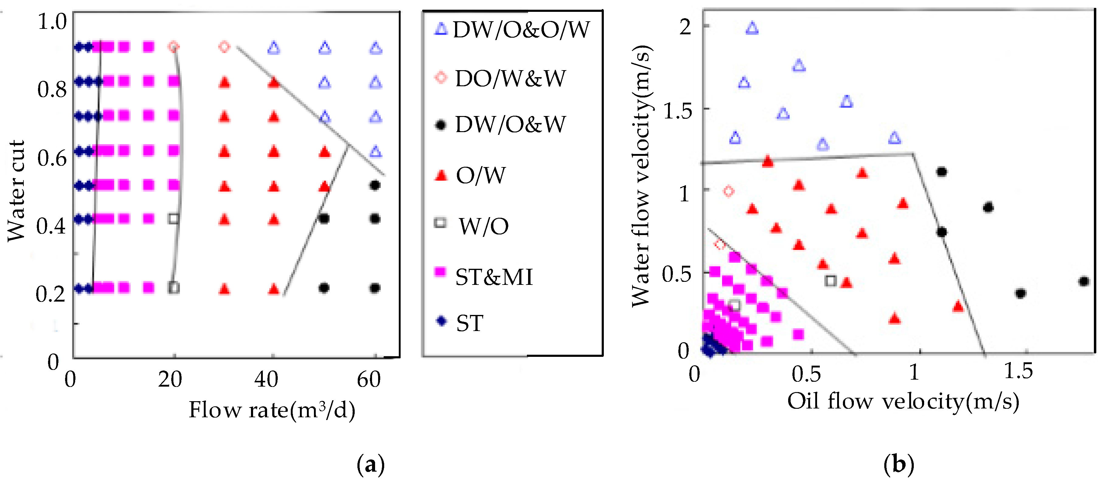
It is necessary to understand the flow characteristics of horizontal oil–water two-phase flow for the water cut measurement. In the process of horizontal profile logging, the fluid exists in the flow state of low yield liquid and high water cut. In this case, because of the difference of oil and water density, the mixture of oil and water exists in the form of a segregated flow. There are many early studies on the flow pattern of horizontal oil–water two-phase flow. Russell et al. [6], Charles et al. [7], Hasson et al. [8], and Trallero et al. [9] carried out the experiment with a horizontal pipe to obtain the flow patterns. Brauner et al. [10] presented the physical model of oil–water two-phase flow pattern transformation in horizontal pipe. It can be deduced that various complex flow structures in the horizontal oil–water two-phase flow bring new challenges to the design of parameter measurement sensors.

Because the capacitance sensor has the advantages of high sensitivity near the electrode, simple structure, fast response speed, and small flow pattern disturbance, the capacitance sensor is gradually used in liquid holdup measurement of two-phase flows [11,12,13]. The capacitance sensors are divided into two types, invasive capacitance sensors and non-invasive capacitance sensors. For invasive capacitance sensors, Zhai et al. [14] employed a parallel-wire capacitance probe to compose the cross-correlation velocity measurement and found that the sensor was affected by the flow patterns to some extent. Ahmed [15] used capacitance probes to investigate the air-oil slug flow parameters by experiments. Zhao et al. [16] optimized the concave capacitance sensor and found that the concave capacitance sensor has a good response character for dispersion of water in oil (DW/O) flow and dispersion of water in oil and oil in water (DW/O&DO/W) flow in horizontal pipe. Han et al. [17,18] optimized the geometry of the coaxial capacitance sensor (COS) and analyzed the influence of oil bubbles on coaxial capacitance sensors. However, the coaxial capacitance sensor may be submerged in the oil or water phase under the conditions of oil–water two-phase stratified flow, which reduces the resolution of the water cut measurement. When the water cut is more than 0.5, the resolution will be lower, which cannot meet the needs of the actual measurement.

Although the above invasive capacitance sensors have achieved good results in the liquid holdup measurement of oil–water two-phase flow, they are obviously limited to the fluid structure of the horizontal oil–water two-phase segregated flow. For the non-invasive capacitance sensor, Xu et al. [19,20] designed a cylindrical capacitance sensor (CYS) and carried out the experimental study by the sensor. However, the cylindrical capacitance sensor loses its resolution when the flow rate is above 20 m³/d and below 3 m³/d, so the sensor cannot meet the requirements of the water cut measurement in horizontal wells within the application range of the flow rate. The combined capacitance sensor (CCS) is a combination of the cylindrical capacitance sensor and the coaxial capacitance sensor and combines the advantages of both. In this paper, the response characteristics of the CCS under different oil–water two-phase flow patterns were analyzed by simulation and experiments, which verified the validity of the CCS.

2. Measuring Principle

2.1. Measurement Principle of the Coaxial Capacitance Sensor

The coaxial capacitance sensor consists of a center electrode and an outer electrode, that is, the metal shell. The center electrode on the central line of the pipe is coated with an insulating layer as shown in Figure 1. The outer electrode is in contact with the fluid and forms a capacitance with the center electrode. When oil and water phases flow between the two electrodes, the capacitance values are different due to the different dielectric constant of oil and water, so the change of capacitance value can indicate the change of the water cut.

When the oil cut is high, the oil is used as the continuous phase in the fluid, and the dielectric property of the fluid is weak. At this time, the entire flow runner is basically insulated, and the sensor has the greatest capacitance value. When the water cut is high, the capacitance of the coaxial capacitance sensor is mainly determined by the size and quantity of the oil bubble near the central electrode. However, the reaction is not obvious for the oil bubble farther away from the central electrode, that is, when the water cut is high, the size, quantity, and distribution of the oil bubble will affect the measurement effect of the sensor.

2.2. Measurement Principle of the Cylindrical Capacitance Sensor

The cylindrical capacitance sensor as shown in Figure 2, is made up of a metal shell, an outer insulating layer, a metal electrode, and an inner insulating layer. The metal electrode is excited by voltage and sealed to insulate the shell and leads to the wire. The metal case is grounded. The fluid flows along the axis in the runner. While ensuring the response strength is measured by the sensor, in order to facilitate the stratified flow of the fluid and increase the measurable range of the fluid, it is necessary to increase the width of the runner so that the thickness of each layer is as small as possible. Moreover, the thinner the internal insulation layer, the wider the response range of the sensor.

Obviously, the metal electrode, the outer insulating layer, and the metal shell form a capacitance C0 in the cylindrical capacitance sensor. When the oil–water two-phase flow is stratified in the sensor runner, because the density of oil is smaller than that of water, oil is in the upper layer of water. The metal electrode, the inner insulating layer, and the water surface in contact with the inner insulating layer form a capacitance C1. The metal electrode, inner insulating layer, oil, and water surface form another capacitance C2. The total capacitance of the cylindrical capacitance sensor is connected in parallel with the above three parts. It can be seen that the cylindrical capacitance sensor is mainly focused on the fluid in the oil–water stratified state, but it is difficult to guarantee an effect when the fluid is in the non-stratified state.

2.3. Measurement Principle of the Combined Capacitance Sensor

The designed CCS in this paper is a combination of the cylindrical capacitance sensor and the coaxial capacitance sensor. As shown in Figure 3, the center electrode of the coaxial capacitance sensor is placed at the center of the cylindrical capacitance sensor, which is in parallel with the metal layer of the cylindrical capacitance sensor. Both of them are electrodes. The shell of the sensor is grounded and the fluid flows in the annular region. For the CCS, the cylindrical capacitance sensor and the coaxial capacitance sensor act together and compensate each other, which increases the response range of the sensor in the state of stratified flow. The effective contact area between the oil bubble and the sensor is increased and the adhesion rate of the oil bubble is increased under the condition of non-stratified flow, thus improving the resolution of the sensor. In Figure 3, R₀, R₁, R₂, R₃, R₄, and R₅ are center electrode radius, insulating layer radius, flow runner radius, inner insulating layer radius, metal electrode radius, and outer insulating layer radius, respectively. L is the length of the sensor. α, β is the center angle of the circle with the radius of R₁, R₂ and oil–water interface, respectively.

When the fluid is in the oil–water two-phase segregated flow, the total capacitance of the CCS is made up of five-part capacitors in parallel. The capacitance formed by the center electrode, metal electrode, and outer insulating layer is recorded as C0. The capacitance formed by the central electrode, the inner insulating layer, and the water in contact with the inner insulating layer is recorded as C1. The capacitance produced by the edge effect of C1 near the interface is denoted by C2. The capacitance formed by the central electrode, insulating layer, and water in contact with the insulating layer is recorded as C3. The capacitance produced by the edge effect of C3 near the interface is denoted by C4.

$$\mathrm{C}0=\frac{2\mathsf{\pi }\mathsf{\epsilon }{\mathsf{\epsilon }}_0\mathrm{L}}{\ln ({\mathrm{R}}_5/{\mathrm{R}}_4)}$$

(1)

$$\mathrm{C}1=\frac{\mathsf{\beta }\mathsf{\epsilon }{\mathsf{\epsilon }}_0\mathrm{L}}{\ln ({\mathrm{R}}_3/{\mathrm{R}}_2)}$$

(2)

$$\mathrm{C}2=\frac{4\mathsf{\beta }\prime \mathsf{\epsilon }{\mathsf{\epsilon }}_0\mathrm{L}}{\ln (\mathrm{R}\prime /{\mathrm{R}}_0)}({\mathrm{Y}}_{\mathrm{w}}-{{\mathrm{Y}}_{\mathrm{w}}}^2)$$

(3)

$$\mathrm{C}3=\{\begin{array}{cc}0& \mathsf{\beta }\le 2\arccos ({\mathrm{R}}_1/{\mathrm{R}}_2)\\ \frac{\mathsf{\alpha }\mathsf{\epsilon }{\mathsf{\epsilon }}_0\mathrm{L}}{\ln ({\mathrm{R}}_1/{\mathrm{R}}_0)}& 2\arccos ({\mathrm{R}}_1/{\mathrm{R}}_2)<\mathsf{\beta }<2\mathsf{\pi }-2\arccos ({\mathrm{R}}_1/{\mathrm{R}}_2)\\ \frac{2\mathsf{\pi }\mathsf{\epsilon }{\mathsf{\epsilon }}_0\mathrm{L}}{\ln ({\mathrm{R}}_1/{\mathrm{R}}_0)}& \mathsf{\beta }\ge 2\mathsf{\pi }-2\arccos ({\mathrm{R}}_1/{\mathrm{R}}_2)\end{array}$$

(4)

$$\mathrm{C}4=\{\begin{array}{cc}\frac{\mathsf{\beta }\mathsf{\epsilon }{\mathsf{\epsilon }}_0\mathrm{L}}{\ln (\mathrm{R}″/{\mathrm{R}}_0)}& \mathsf{\beta }\le 2\arccos ({\mathrm{R}}_1/{\mathrm{R}}_2)\\ \frac{\mathsf{\beta }\mathsf{\epsilon }{\mathsf{\epsilon }}_0\mathrm{L}(1-\mathsf{\alpha }/2\mathsf{\pi })}{\ln (\mathrm{R}\prime /{\mathrm{R}}_0)}& 2\arccos ({\mathrm{R}}_1/{\mathrm{R}}_2)<\mathsf{\beta }<2\mathsf{\pi }-2\arccos ({\mathrm{R}}_1/{\mathrm{R}}_2)\\ \frac{\mathsf{\beta }\mathsf{\epsilon }{\mathsf{\epsilon }}_0\mathrm{L}(2\mathsf{\pi }-\mathsf{\alpha })}{2\mathsf{\pi }\ln (\mathrm{R}\prime /{\mathrm{R}}_0)}& \mathsf{\beta }\ge 2\mathsf{\pi }-2\arccos ({\mathrm{R}}_1/{\mathrm{R}}_2)\end{array}$$

(5)

where, $\mathsf{\epsilon }$ is the dielectric constant of the vacuum state, and ${\mathsf{\epsilon }}_0$ is the dielectric constant of the insulating layer, the inner and outer insulating layer, and oil. ${\mathrm{Y}}_{\mathrm{w}}$ is the water cut of fluid. $\mathrm{R}\prime =({\mathrm{R}}_1+{\mathrm{R}}_2)/2$. $\mathrm{R}″=[{\mathrm{R}}_2+{\mathrm{R}}_2\cos (\mathsf{\beta }/2)]/2$. $\mathsf{\beta }\prime =2\arccos ({\mathrm{R}}_1/{\mathrm{R}}_2)$.

The total capacitance of CCS is the sum of C0, C1, C2, C3, and C4. It can be seen from the formulas that the capacitance of CCS is corresponding to the water cut of the fluid, which can reflect the water cut of the horizontal oil–water two-phase segregated flow.

3. Simulation and Analysis

Based on the structure model of the CCS in Figure 3, the electric field can be formed between exciting and measuring electrodes through voltage excitation. Because of the complicated nature, it is difficult to establish a function to describe the relationship between sensor output and sensor parameters. Thus, finite element analysis [21,22,23] was used to calculate the sensor responses.

For a given dielectric distribution, electrode configuration, and boundary conditions, the potential of the sensor can be calculated by solving Poisson’s equation:

$${\nabla }^2\phi =-\frac{\rho }{\epsilon }.$$

(6)

For the three-dimensional electric field:

$$\begin{array}{cc}\frac{{\partial }^2\phi }{\partial x^2}+\frac{{\partial }^2\phi }{\partial y^2}+\frac{{\partial }^2\phi }{\partial z^2}=-\frac{\rho (x,y,z)}{\epsilon (x,y,z)}& \phi =\phi (x,y,z)\end{array}$$

(7)

where $\phi$ is the space potential distribution function, $\rho$ refers to the space charge density, $\epsilon$ represents the space permittivity distribution function. If there is no free charge in the measurement field ($\rho =0$), Equation (6) can be calculated by ${\nabla }^2\phi =0$. Thus, the capacitance values can be obtained by the finite element method.

The normalized capacitance values denoted by C_N were used to analyze the static response characteristics of the CCS, and can be calculated by

$${\mathrm{C}}_{\mathrm{N}}=\frac{{\mathrm{C}}_{\mathrm{w}}-\mathrm{C}}{{\mathrm{C}}_{\mathrm{w}}-{\mathrm{C}}_{\mathrm{o}}}$$

(8)

where ${\mathrm{C}}_{\mathrm{w}}$ and ${\mathrm{C}}_{\mathrm{o}}$ are the capacitance response values of sensors in the pure water phase and the pure oil phase, and C is the capacitance response values of sensors under different flow patterns. The response resolution of the sensor was analyzed by obtaining the curve of normalized capacitance value C_N with the water cut. Obviously, the greater the curve slope, the better the resolution of the sensor.

The employed geometry of the CCS was: R₀ = 4 mm, R₁ = 5 mm, R₂ = 13 mm, R₃ = 14 mm, R₄ = 15 mm, R₅ = 19 mm, L = 100 mm. The CCS was modeled and meshed by COMSOL simulation software, and the tetrahedron mesh was used to divide it. The relative dielectric constant of oil and insulating material was set as 3.5. The relative dielectric constant of water was set as 80. The relative dielectric constant of the metal material was set as 1000. The voltage of the center electrode and the metal electrode was set to 10 V, and the shell and water were grounded. Furthermore, the dependency of the CCS model on the number of the meshed grids in the finite model was investigated. Under the conditions that the CCS was in a pure oil phase, the simulation results of the CCS for different mesh numbers are listed in

Table 1. Capacitance values of the combined capacitance sensor (CCS) with different grids.

No.	Total Grids	Maximum Unit Size (mm)	Minimum Unit Size (mm)	Capacitance Values (F)
1	43,952	10	3.5	4.3235 × 10−10
2	60,352	10	2.5	4.3237 × 10−10
3	145,827	9	2	4.3238 × 10−10
4	228,374	8	1.5	4.3237 × 10−10
5	229,413	7	0.3	4.3237 × 10−10

. As shown in Table 1, it is obvious that the capacitance values of the CCS have very small differences in different grids, which indicates the relative independence of the calculated results on the meshed grids. Considering that the calculation speed and accuracy were not affected, the number 228,374 was selected to be the optimal number of elements for CCS simulation in this paper.

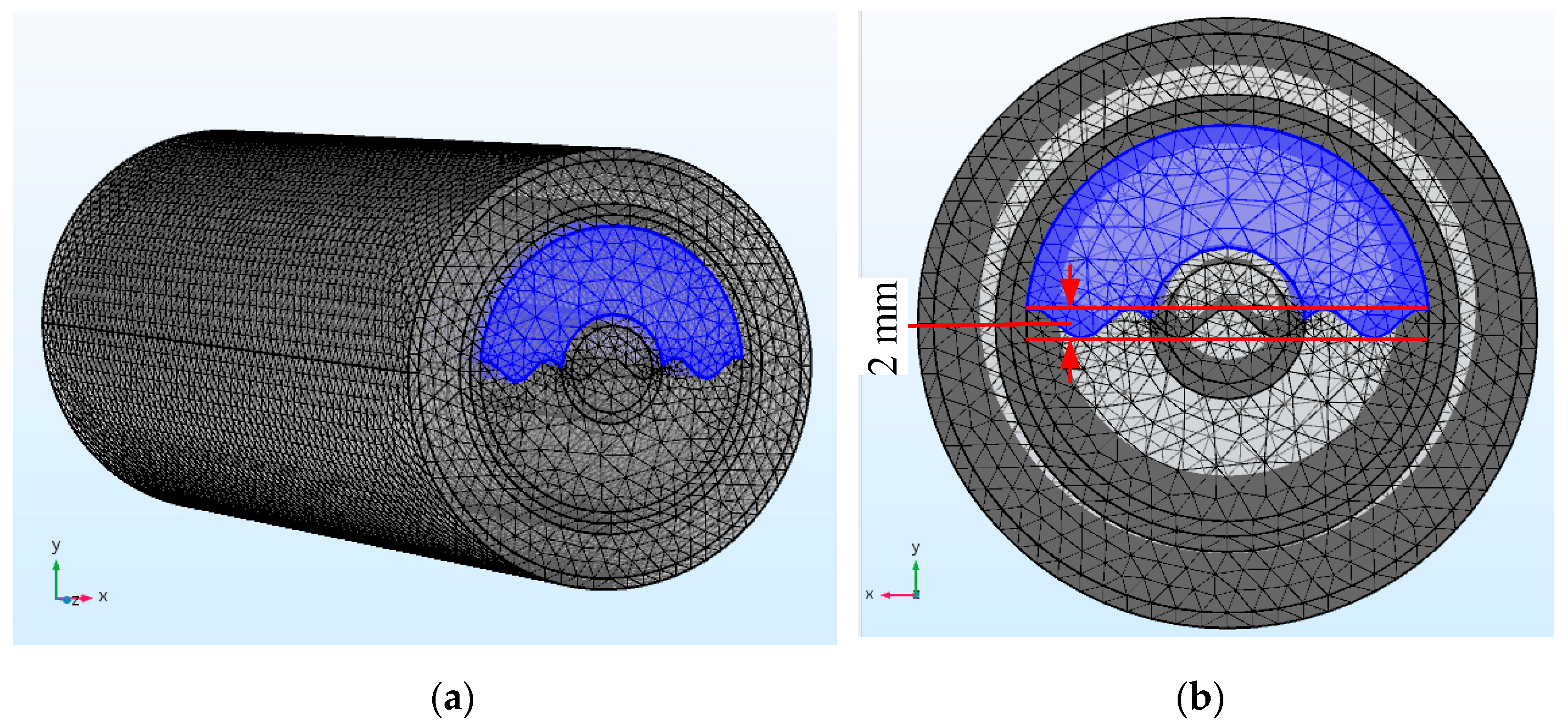
In order to obtain the response characteristics of CCS under different flow patterns, the finite element models of six flow patterns, including stratified flow (ST), stratified flow with mixing at the interface (ST&MI), dispersed flow that includes dispersion of oil in water and water flow (DO/W&W), oil in water emulsion (O/W), dispersion of water in oil and oil in water flow (DW/O&DO/W), and water in oil emulsion (W/O), which were proposed by Trallero et al. [9], were constructed. For ST flow patterns, the meshed model of the CCS is shown in Figure 4, where the blue color represents the oil phase and the area outside the annular runner represents the water phase for the ST flow pattern. In Figure 4, the water cut is 0.6.

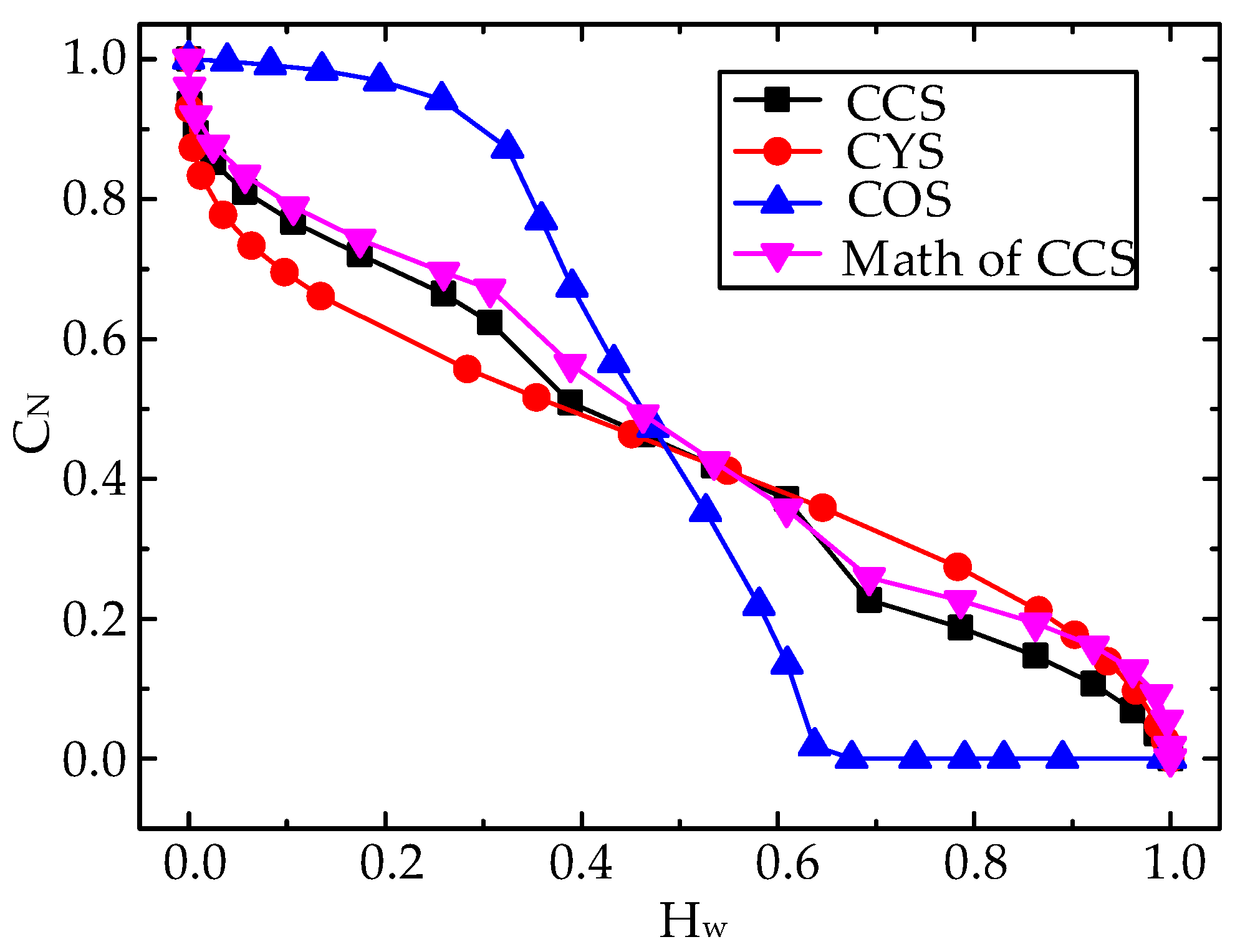
In order to better analyze the static response characteristics of the CCS, the sensors CYS and COS were modeled and simulated. Because the CCS is the combination of the CYS and the COS, the CYS and the COS were simulated with the same structural parameters and simulation conditions as the CCS. Using COMSOL simulation software, the static response curves of the CCS, CYS, and COS under the ST flow pattern were calculated by the finite element method as shown in Figure 5, where the math of the CCS represents the results calculated by the measurement principle of the CCS. As can be seen from the figure, the static response values of the CCS were basically consistent with the results obtained through the mathematical model, and the C_N decreased with the increase of the water cut. The reason for the slight difference between the simulation results and the results calculated by the mathematical model is that in the mathematical model of the CCS, the capacitance C3 and C4 introduced by the boundary effect near the oil–water interface were approximately calculated. Compared with the CYS, the slope of the result curve of the CCS in the water cut range 0~0.4 and 0.6~1 increases obviously, which indicates that the resolution oil of the CCS was better under an ST flow pattern. The COS has no response when the water cut was greater than 0.63. The reason is that when the oil–water interface exceeds the center electrode, the oil phase cannot contact the electrode, so the response value of the COS will not change. The results show that the CCS has better resolution abilities compared with the CYS and the COS for the ST flow pattern.

Figure 6 shows the mesh model of the CCS for the ST&MI flow pattern, where the water cut is 0.5058, the blue color represents oil, and the area outside the annular runner represents water. In order to construct the ST&MI flow pattern, the wave of flow pattern was represented by a sinusoidal curve with a peak value of 1 mm, which represents the wave height of the interface.

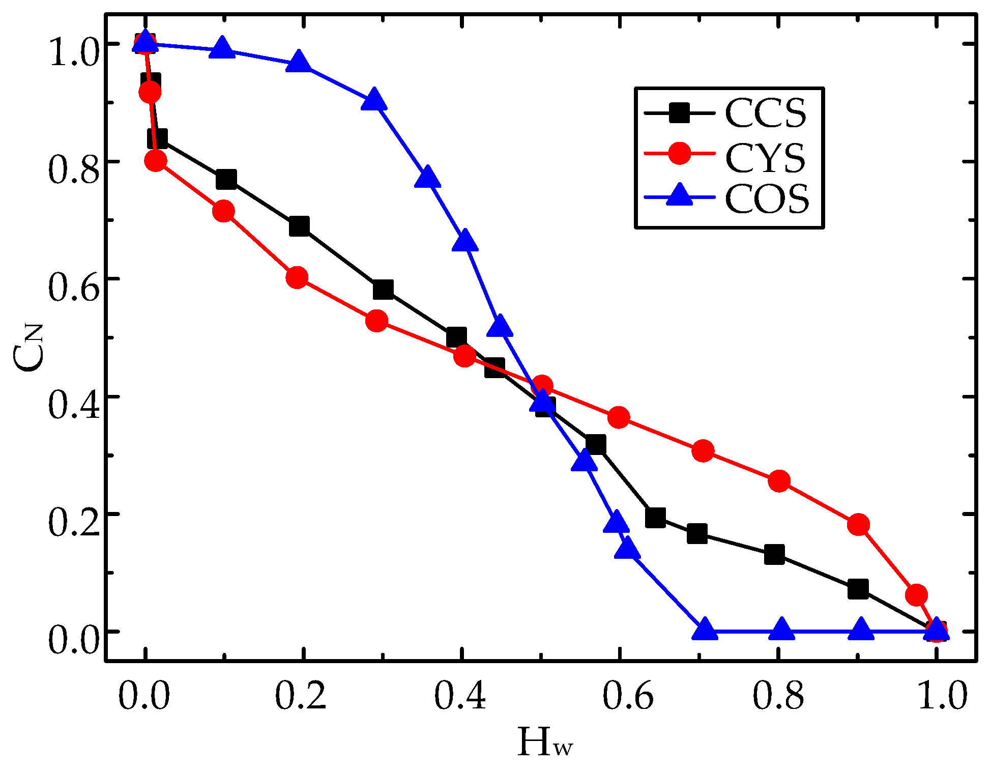
The static response curves of the CCS, CYS, and COS under an ST&MI flow pattern were calculated as shown in Figure 7. As observed from the figure, the variation trends of the three sensors are approximately the same as the response curves under an ST flow pattern. With the increase of the water cut, the response values decreased. Due to the structural characteristics of fluid fluctuations for the ST&MI flow pattern, the response curve is slightly less smooth than the ST flow pattern. Compared with the response values of the CYS and the COS, the CCS had better response characteristics, which shows that the combined capacitance sensor has a good resolution ability for ST&MI flow patterns with different water cuts.

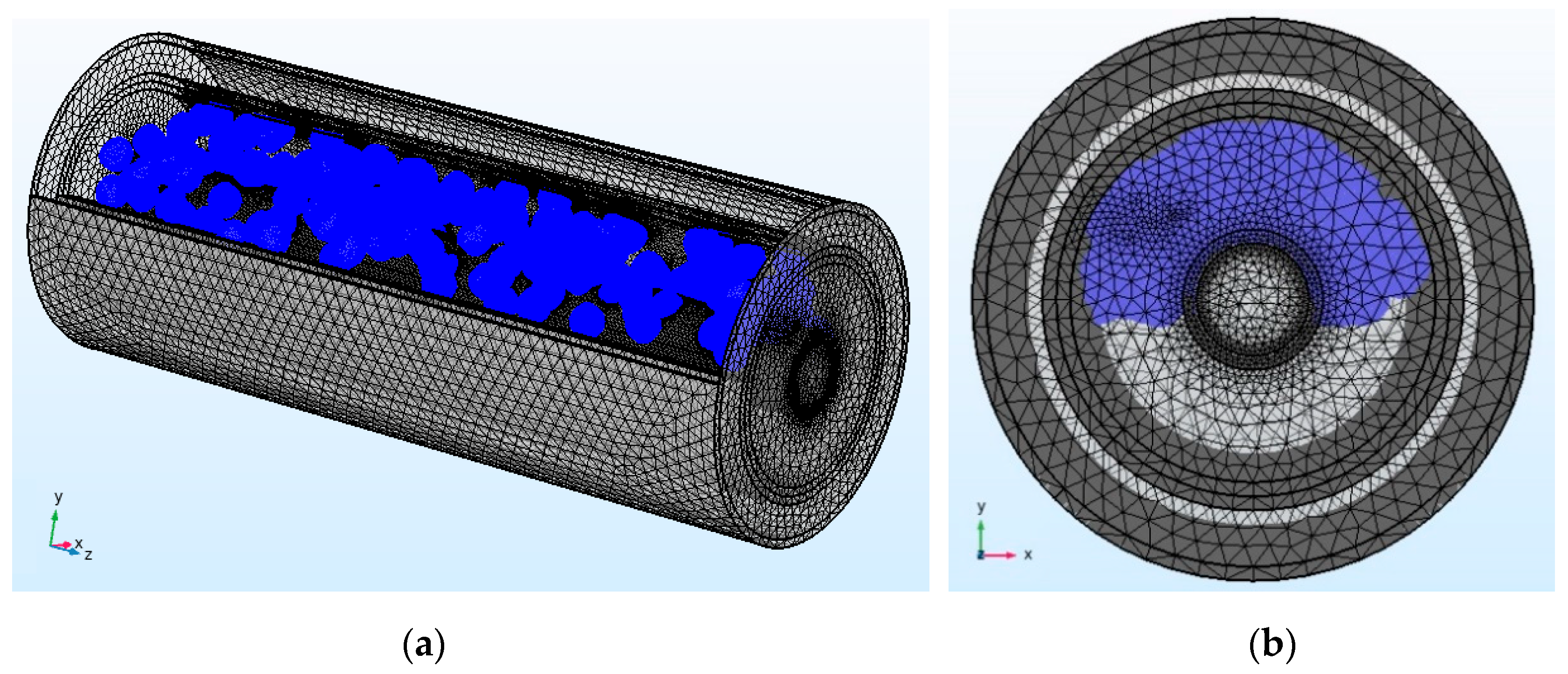
The mesh model of the CCS for the DO/W&W flow pattern is shown in Figure 8, where the water cut is 0.8907. In the process of constructing the model, in the upper water phase, the oil droplets with the same radius of 0.2 mm were randomly distributed in different axial and radial cross sections. The initial number of oil droplets was 200. The water cut was changed by changing the quantity of oil droplets. Because of the uneven distribution of oil droplets, the mesh model was encrypted. Figure 8a shows the relative position of the oil droplet to the center electrode, and Figure 8b is the 2D model of the XOY section under the DO/W&W flow pattern.

Figure 9 shows the static responses of the CCS, CYS, and COS for the DO/W&W flow pattern under different water cuts. Obviously, with the increase of the water cut, all response values showed a downward trend. From the analysis of the figure, the sensor resolution of the COS was the largest among the three sensors. The resolution of the CCS was greater than that of the CYS under the DO/W&W flow pattern. The variety of sensor response values was due to the oil droplets that attached to the electrode led to the variety of the thickness of the insulating layer between the sensor electrodes, so the response value of the sensor was changed. Moreover, the CCS had two electrodes to contact fluids, and oil droplets were more likely to attach to the sensor electrodes, which resulted in higher resolution of the CCS than that of the CYS. In addition, the non-smooth response curve of the sensor was mainly caused by the random distribution of the oil bubble, which better reflects the real situation of the actual measurement.

For the O/W flow pattern, the mesh model was constructed as shown in Figure 10, where the water cut is 0.795. The model was constructed similar to that of the DO/W&W flow pattern. The difference was that oil droplets of the same radius were also randomly distributed in the lower layers of the fluid. The initial number of oil droplets was 400. The water cut was changed by changing the quantity of oil droplets. The grid of the model was also encrypted. Figure 10a shows the relative position of oil droplets and the center electrode, and Figure 10b is the 2D model of the XOY section under the O/W flow pattern.

The static responses of the CCS, CYS, and COS for the O/W flow pattern under different water cuts are shown in Figure 11. It can be seen from the figure that the response result of the DO/W&W flow pattern is similar to that of the O/W flow pattern. Likewise, the CCS and the COS have greater resolution than the CYS for the O/W flow pattern.

Because of the complexity of the DW/O&DO/W flow pattern, the simplified model was used to simulate the DW/O&DO/W flow pattern. Figure 12 shows the finite element model for the DW/O&DO/W flow pattern with a water cut of 0.5543. The upper part of the runner was evenly distributed in the continuous oil phase, and the lower part of the flow runner was distributed in the continuous water phase. The oil–water interface was composed of sinusoidal curves with a peak value of 1 mm. By changing the oil droplet size in the continuous water phase and the water droplet size in the continuous oil phase, the capacitance value of the CCS for the DW/O&DO/W flow pattern can be measured under different water cut conditions. Figure 12a shows the relative position of the lower layer to the oil droplets with a radius of 1mm, in which the number of radial sections of the droplets was 20, each radial segment consisted of four oil droplets, and the total number of droplets in the continuous water phase was 80. Figure 12b shows the relative position of the upper layer and the water droplets with a radius of 1mm, in which the number of radial sections of the droplets was 20, each radial portion included 12 droplets, and the total number of drops in the continuous oil was 240. Figure 12c shows the 2D model of the XOY section under the DW/O&DO/W flow pattern.

The static responses of the CCS, CYS, and COS for the DW/O&DO/W flow pattern were simulation calculated as shown in Figure 13. As observed from the figure, the static response values of the CCS, CYS, and COS decreased with the increase of the water cut. The downward trend of the CCS simulation results were more consistent with that of the CYS, while the slope of the response curve of the COS was larger, which indicates that the COS has better resolution ability for DW/O&DO/W flow patterns. Furthermore, the CCS also has a certain resolution for DW/O&DO/W flow patterns.

Figure 14 shows the mesh model of the CCS for the W/O flow pattern with the water cut of 0.1759. In order to realize the uniform distribution of water droplets in the continuous oil phase, the isometric water droplets were placed in the axial direction. The water cut was changed by changing the radius of the water droplet. Figure 14a shows the relative position of the water droplet and the center electrode, in which eight water droplets were placed in different radial positions in the same axial position and 20 oil droplets in different axial positions in the same radial position. Figure 14b shows the 2D model of the XOY section under the W/O flow pattern.

The static responses of the CCS, CYS, and COS for the W/O flow pattern under different water cuts are shown in Figure 15. It can be seen from the figure that with the increase of the water cut, the static response values of the CCS, CYS, and COS decreased. The variation trend of the CCS and the COS was consistent, and the slope of the CYS response curve was smaller, which indicates that the CCS and the COS have a better resolution ability compared with the CYS for the W/O flow pattern under different water cuts.

In summary, for the six flow patterns of horizontal oil–water two-phase flow, although the COS shows a good resolution in some flow patterns, it has no resolution when the water cut is larger than 0.7 under ST and ST&MI flow patterns. Thus, the COS has difficulty meeting the conditions of low-yield horizontal wells. The CCS shows a good resolution under six flow patterns and is superior to the CYS. Therefore, the CCS combines the advantages of the CYS and the COS.

4. Experiments and Analysis

4.1. Experimental Facility

The CCS consists of a cylindrical metal layer electrode and a central electrode rod in parallel in circuit, which are both sensitive to the change of the retention rate of oil and water components in the flow runner space, as shown in Figure 16. The ring space between the inner wall of the metal electrode and the built-in electrode rod is the flow runner of the combined capacitance sensor, that is, the fluid flow region. The photo of the CCS we made is shown in Figure 17. The polyimide was used as the insulating layer.

In order to verify the effectiveness of the CCS in practical measurement, a dynamic experiment was carried out on a horizontal oil–water two-phase flow experimental facility in the Petrodaqing Test and Experiment Center of Logging and Testing Technology. The flow experimental facility is shown in Figure 18, which consisted of a water tank, an oil tank, a separation tank, two horizontal peristaltic metering pumps, two plexiglass testing pipes with a diameter of 125 mm and 20 mm, a high-speed camera, and the combined capacitance instrument. The pipe with the diameter of 125 mm was used to measure the water cut using the combined capacitance instrument. The pipe with the diameter of 20 mm was used to observe the flow pattern using the high-speed camera. The combined capacitance instrument was made up of the CCS, the umbrella-type flow collector, and the circuit. In the measurement, the fluid including oil and water phases was collected by the umbrella-type flow collector and flowed into the CCS. The Swiss MacroVis high-speed camera named SpeedCam was used in the experiment. A CMOS color sensor was built into the camera. Full resolution recording time was 3.3 s. When the maximum dynamic output pixel is 1280 × 1024, the picture update rate is 1000 frames/s, and when the minimum output pixel is 1280 × 10, the picture update rate can reach 93,282 frames/s. In this experiment, according to the velocity of flow, the frame rate was set from 2100 frames/s to 3000 frames/s, and the output pixels range from 1280 × 350 to 1280 × 500.

In the experiment, water from the water tank and oil from the oil tank through peristaltic metering pumps were pumped into the plexiglass testing pipe. The mixed fluid was collected through the umbrella-type collector and flowed into the CCS to measure the water cut. Then the fluid passed through the plexiglass pipe with the diameter of 20 mm and was photographed by the high-speed camera to obtain the flow pattern. Finally, the mixed fluid flowed into the separation tank and was separated by density difference, so that it could be recycled. The experimental medium was tap water and D110 white oil. The density of water is 1 g/cm³, and the density of D110 white oil is 0.825 g/cm³. The reason for the use of tap water is that due to the long-term water injection development in Daqing Oilfield, the mineralization degree of oilfield brine is reduced from 6000 to 2000 ppm, which is basically the same as that of tap water. Thus, the small difference between tap water and brine has little effect on the results.

Considering that the measurement results of the instrument were influenced by the repeatability errors of measurement and system errors for long time continuous operation, the horizontal oil–water two-phase flow experimental facility was used to carry out the segregated flow experiments multiple times using the experimental point where the flow rate was set as 3, 5, 10, 15, 20~60 m³/d by a step of 10 m³/d, and the water cut was set as 0~1 by a step of 0.1.

4.2. Calibration Experiments under Different Temperatures and Pressures

Since the temperature and pressure of oilfield fluid is different from that on the ground, the calibration experiments were first carried out to investigate the response characteristics of the CCS under different temperatures and pressures.

In the calibration experiment of temperature, the CCS was placed in an oil-filled or water-filled measuring cup in the oven. The temperature of oil was raised to 125 °C, and the temperature of water was adjusted to 80 °C. The capacitance values of the CCS were measured under different temperatures in the oil and water, respectively. The calibration results are listed in

Table 2. Calibration results of the CCS in the pure oil phase at different temperatures.

Oil temperature (°C)	20	80	100	125
Capacitance values (μF)	120	118	116	119

and

Table 3. Calibration results of the CCS in the pure water phase at different temperatures.

Water temperature (°C)	20	60	80
Capacitance values (μF)	390	392	394

. From the analysis of the results, the capacitance values of the CCS in the pure water phase are obviously larger than that in the pure oil phase, which was consistent with the simulation results. Moreover, the capacitance value of the CCS does not change obviously at different temperatures, which shows that the CCS has a good temperature performance.

In the calibration experiment of pressure, the combined capacitance instrument was put into the pressure simulation well filled with diesel oil in the Petrodaqing Test and Experiment Center of Logging and Testing Technology. The pressure was set as 15, 25, and 40 MPa. The calibration results were obtained and listed in

Table 4. Calibration results of the CCS instrument in the pure oil phase at different pressures.

Pressure (MPa)	Normal	15	25	40
Frequency values (Hz)	1744	1750	1754	1766

. It can be seen from the results that with the increase of pressure, the frequency response values had the tendency to increase slightly, but the change was not obvious. The maximum deviation of the response value was not more than 1.2%, which verifies the pressure stability of the instrument.

4.3. Flow Pattern Analysis under Different Working Conditions

Seven flow patterns were obtained using a high-speed camera, as shown in Figure 19. Stratified flow (ST) is shown in Figure 19a. The oil–water interface is clear, and the boundary line is a straight and smooth wave line. This flow pattern occurs at low velocity of the oil–water mixture, and gravity and buoyancy play leading roles. For the stratified flow with mixing at the interface (ST&MI) as shown in Figure 19b, the interface between oil and water is obvious and irregular. With the increase of the velocity of the oil–water mixture and the difference of the oil–water viscosity, during the development of the flow pattern, the difference of the oil–water velocity resulted in a particularly obvious fluctuation in the interface, but no obvious droplets were formed. For dispersed flow that includes dispersion of oil in water and water flow (DO/W&W), as shown in Figure 19c, in aqueous solution, there are some oil bubbles or slug in the upper part of the pipe. The bottom is water. Figure 19d is the oil in water emulsion (O/W), where oil is dispersed in water by oil bubbles and slug-shaped large oil bubbles. Water in oil emulsion and oil in water emulsion (DW/O&O/W), is shown in Figure 19e. When the water cut is low, the water phase exceeds the bearing capacitance of the oil phase with the increase of the flow velocity, and some oil droplets are dispersed in the water. For water in oil and water flow (DW/O&W), as shown in Figure 19f, when the flow rate of oil and water is low and the oil cut in the oil/water mixture is high, some water droplets in the oil phase are distributed in the upper layer of the pipe, and the water phase is distributed in the lower layer of the pipe due to gravity action. Water in oil (W/O) is shown in Figure 19g. Water is in the dispersed phase, and oil is in the continuous phase. It mainly occurs in the flow conditions of high flow and low water cut, where the water phase is dispersed into droplets and evenly dispersed in oil.

The distributions of different flow patterns with a flow rate and a water cut were obtained experimentally, as shown in Figure 20a. The flow pattern distribution of the oil and water phase velocity calculated by flow rate and water cut is shown in Figure 20b. From the figure, we can clearly obtain the relationship between the flow pattern of the horizontal oil–water two-phase flow and the flow rate, water cut, and the velocity of each phase. Through the analysis of the flow patterns of the horizontal oil–water two-phase flow, the response characteristics of capacitance sensors under different flow patterns can be obtained experimentally.

4.4. Analysis of Dynamic Experiment Results

In order to obtain a reliable measurement value, the output response of the instrument under different flow rates and water cuts was recorded. The output frequency value was used to reflect the capacitance value of the CCS, and the capacitance value had a certain relationship with the water cut. Thus, the frequency was used to calibrate the water cut. The frequency values obtained from the CCS in the pure water phase and the pure oil phase are listed in

Table 5. Frequency values obtained from the CCS under conditions of a pure water phase and a pure oil phase.

	Pure Water Phase	Pure Oil Phase
Frequency values (Hz)	224	1918

. It can be seen that the frequency value obtained from the CCS in the pure oil phase is larger than that in the pure water phase, which is consistent with the results of the simulation as shown in Figure 5.

The frequency signal from the CCS with the flow rate of 30 m³/d varies with time as shown in Figure 21. As observed from the figure, the frequency values decrease with the increase of the water cut, which was consistent with the simulation results of the CCS. In addition, it can be seen preliminarily that the higher the water cut, the more stable the frequency.

In order to be more conducive to the comparison of values, the output frequency of the instrument was standardized by that of the pure oil phase and the pure water phase to obtain the standardized response. Figure 22 shows the response law of the instrument under different flow rates and water cuts. It can be seen from the figure that when the flow rate is 3~60 m³/d, and the water cut is 0~1, the instrument has a response characteristic. When the water cut is less than 0.2, the trend of the CCS response curve is relatively smooth. When the water cut reaches 0.3, the response values of the CCS become larger, especially when the flow rate is greater than 40 m³/d. This is because when the water content is greater than 0.3, the height of the oil–water interface reaches the boundary of the central electrode rod of the CCS. In this case, the capacitance of the sensor was more easily affected by the electrode rod, which was consistent with the simulation results. When the flow rate increased, the oil–water interface at the central electrode rod became more unstable. Additionally, the more susceptible the CCS was to the electrode rod, the greater the change of response value.

The CCS was designed to measure the water cut under different flow rates. When measuring the water cut with the CCS, the flow rate of fluid is known. According to the flow rate of the fluid and the response value of the CCS as shown in Figure 22, the water cut of the fluid can be obtained. Thus, for a certain flow rate, the CCS has response characteristics under different water cuts, which indicates that the CCS can effectively measure the water cut. Although the resolution decreases below 10 m³/d and decreases to the minimum at 3 m³/d, it still has resolution and is better than the conventional coaxial and cylindrical capacitance sensors. In addition, because different flow patterns will appear at a certain flow rate in the dynamic experiments, it is difficult to obtain the corresponding flow pattern and the result curve of the simulation experiment. Nevertheless, it can be seen from the figure that for different flow patterns, the CCS has a good resolution, which shows that the calibration results of the CCS were consistent with the simulation results.

In order to obtain the fluctuation trend of the CCS under different working conditions, through setting parameters, a specified number of frequency values were sampled in a certain time using the instrument. In addition, the standard deviation [24,25] of all frequency numbers from each flow rate and water cut point was obtained. The standard deviation of each flow rate and water cut point was interpolated to obtain the 3D map, as shown in Figure 23.

As can be seen from the figure, when the flow rate is 10~60 m³/d, the fluctuation of CCS responses is very small, and the flow rate and water cut have little effect on it. When the flow rate is 60 m³/d and the water cut is 0.3~0.4, the standard deviation tends to increase. It can be deduced that in this case, the oil and water emulsifies, a large number of continuous water flows into the instrument, and the conduction current in the fluid increases sharply. Thus, the random fluctuation also increases, and the response volatility becomes larger. In addition, when the maximum standard deviation of the sensor appears at a low flow rate, it is considered that the oil bubble is large in volume and unevenly distributed in the water phase at this time. At the same time, due to the influence of the hydrophilicity of the insulating dielectric layer on the electrode surface, the oil-covered electrode or the departure electrode is accidental, so the response standard deviation is large.

5. Conclusions

This paper was devoted to analyzing the response characteristics of the CCS for oil cut measurement in the horizontal oil–water two-phase flow. By using the finite element method, the static response characteristics of the CCS, CYS, and COS were obtained. The simulation results show that the CCS was better than the other two sensors in measuring the water cut for different flow patterns. The temperature and pressure calibration experiments of the CCS were conducted. The calibration results show that the CCS has a good stability under different temperatures and pressures. The dynamic experiment was carried out on the horizontal oil–water two-phase flow experimental facility under different working conditions. The flow pattern distribution of the horizontal oil–water two-phase flow with different flow rates and water cuts was obtained by high-speed camera. The response values of the CCS were obtained under different flow pattern conditions, which show that the CCS has good response characteristics in the range of flow rate 3–60 m³/d. It can be deduced that the CCS can be effectively applied in the water cut measurement in the horizontal oil–water two-phase flow.

References

1. Edomwonyi-Otu, L.; Angeli, P. Pressure drop and holdup predictions in horizontal oil-water flows for curved and wavy interfaces. Chem. Eng. Res. Des. 2015, 93, 55–65. [Google Scholar] [CrossRef]
2. Zhai, L.S.; Angeli, P.; Jin, N.D.; Zhou, D.S.; Zhou, L. The nonlinear analysis of horizontal oil-water two-phase flow in a small diameter pipe. Int. J. Multiph. Flow 2017, 92, 39–49. [Google Scholar] [CrossRef] [Green Version]
3. Kong, W.; Kong, L.; Li, L.; Liu, X.; Cui, T. The influence on response of axial rotation of a six-group local-conductance probe in horizontal oil-water two-phase flow. Meas. Sci. Technol. 2017, 28, 065104. [Google Scholar]
4. Wang, Y.; Li, H.; Liu, X.; Zhang, Y.; Xie, R.; Huang, C.; Hu, J.; Deng, G. Novel Downhole Electromagnetic Flowmeter for Oil-Water Two-Phase Flow in High-Water-Cut Oil-Producing Wells. Sensors 2016, 16, 1703. [Google Scholar] [CrossRef] [PubMed]
5. Xie, B.; Kong, L.; Kong, D.; Kong, W.; Li, L.; Liu, X.; Chen, J. Design and numerical simulation on an auto-cumulative flowmeter in horizontal oil–water two-phase flow. Rev. Sci. Instrum. 2017, 88, 115003. [Google Scholar] [CrossRef] [PubMed]
6. Russell, T.W.F.; Hodgson, G.W.; Govier, G.W. Horizontal pipeline flow of mixtures of oil and water. Can. J. Chem. Eng. 2015, 37, 9–17. [Google Scholar] [CrossRef]
7. Charles, M.E.; Govier, G.W.; Hodgson, G.W. The horizontal pipeline flow of equal density oil-water mixtures. Can. J. Chem. Eng. 2015, 39, 27–36. [Google Scholar] [CrossRef]
8. Dong, T.; Ayala, L.F. Two-phase flow models for thermal behavior interpretation in horizontal wellbores. J. Pet. Explor. Prod. Technol. 2016, 6, 45–61. [Google Scholar] [CrossRef]
9. Trallero, J.L.; Sarica, C.; Brill, J.P. A study of oil-Water Flow Patterns in Horizontal Pipes. SPE Prod. Facil. 1997, 12, 165–172. [Google Scholar] [CrossRef]
10. Brauner, N.; Maron, D.M. Flow pattern transitions in two-phase liquid-liquid flow in horizontal tubes. Int. J. Multiph. Flow 1992, 18, 123–140. [Google Scholar] [CrossRef]
11. Goldstein, A.; Ullmann, A.; Brauner, N. Characteristics of stratified laminar flows in inclined pipes. Int. J. Multiph. Flow 2015, 75, 267–287. [Google Scholar] [CrossRef]
12. Jin, B.; Zhang, Z.; Zhang, H. Structure design and performance analysis of a coaxial cylindrical capacitive sensor for liquid-level measurement. Sens. Actuators A Phys. 2015, 223, 84–90. [Google Scholar] [CrossRef]
13. Cui, Z.; Wang, H.; Yin, W. Electrical Capacitance Tomography with Differential Sensor. IEEE Sens. J. 2015, 15, 5087–5094. [Google Scholar] [CrossRef]
14. Zhai, L.S.; Jin, N.D.; Gao, Z.K.; Zhao, A.; Zhu, L. Cross-correlation velocity measurement of horizontal oil–water two-phase flow by using parallel–wire capacitance probe. Exp. Therm. Fluid Sci. 2014, 53, 277–289. [Google Scholar] [CrossRef]
15. Ahmed, W.H. Experimental investigation of air–oil slug flow using capacitance probes, hot-film anemometer, and image processing. Int. J. Multiph. Flow 2011, 37, 876–887. [Google Scholar] [CrossRef]
16. Zhao, A.; Jin, N.D.; Zhai, L.S.; Gao, Z.K. Liquid holdup measurement in horizontal oil–water two-phase flow by using concave capacitance sensor. Measurement 2014, 49, 153–163. [Google Scholar]
17. Zhang, H.; Zhai, L.; Han, Y.; Chen, X.; Gao, Z.; Jin, N. The Response Characteristics of Coaxial Capacitance Sensor for Horizontal Segregated and Non-uniform Oil-Water Two-Phase Flows. IEEE Sens. J. 2017, 17, 359–368. [Google Scholar] [CrossRef]
18. Chen, X.; Han, Y.F.; Ren, Y.Y.; Zhang, H.X.; Zhang, H.; Jin, N.D. Water holdup measurement of oil-water two-phase flow with low velocity using a coaxial capacitance sensor. Exp. Therm. Fluid Sci. 2017, 81, 244–255. [Google Scholar] [CrossRef]
19. Liu, X.; Hu, J.; Xu, W.; Xu, L.; Xie, Z.; Li, Y. A new cylindrical capacitance sensor for measurement of water cut in a low-production horizontal well. J. Phys. Conf. Ser. 2009, 147, 1–7. [Google Scholar] [CrossRef]
20. Xu, W.; Xu, L.; Liu, X.; Hu, J. Experimental study on cylindrical capacitance sensor. In Proceedings of the 2009 IEEE Instrumentation and Measurement Technology Conference (I2MTC), Singapore, 5–7 May 2009; pp. 5–8. [Google Scholar]
21. Xiong, H.; Zhu, X.; Zhang, R. Energy Recovery Strategy Numerical Simulation for Dual Axle Drive Pure Electric Vehicle Based on Motor Loss Model and Big Data Calculation. Complexity 2018, 2018, 4071743. [Google Scholar] [CrossRef]
22. Rosu, L.; Elias-Birembaux, H.L.; Lebon, F. Finite Element Modeling of an Aircraft Tire Rolling on a Steel Drum: Experimental Investigations and Numerical Simulations. Appl. Sci. 2018, 8, 593. [Google Scholar] [CrossRef]
23. Sun, X.; Zhang, H.; Meng, W.; Zhang, R.; Li, K.; Peng, T. Primary resonance analysis and vibration suppression for the harmonically excited nonlinear suspension system using a pair of symmetric viscoelastic buffers. Nonlinear Dyn. 2018, 94, 1243–1265. [Google Scholar] [CrossRef]
24. Han, L.F.; Tang, W.Y.; Liu, Y.M.; Wang, J.; Fu, C.F. Evaluation of measurement uncertainty based on grey system theory for small samples from an unknown distribution. Sci. China Technol. Sci. 2013, 56, 1517–1524. [Google Scholar] [CrossRef]
25. Zhang, R.; He, Z.; Wang, H.; You, F.; Li, K. Study on self-tuning tyre friction control for developing main-servo loop integrated chassis control system. IEEE Access 2017, 5, 6649–6660. [Google Scholar] [CrossRef]
Figure 1. Structure diagram of the coaxial capacitance sensor.
Applsci 09 00346 g001
Figure 2. Structure diagram of the cylindrical capacitance sensor.
Applsci 09 00346 g002
Figure 3. Structure diagram of the combined capacitance sensor.
Applsci 09 00346 g003
Figure 4. Mesh model of the CCS for the stratified flow (ST) flow pattern (a) 3D; (b) XOY section.
Applsci 09 00346 g004
Figure 5. The static responses of the CCS, the cylindrical capacitance sensor (CYS), and the coaxial capacitance sensor (COS) for the ST flow pattern.
Applsci 09 00346 g005
Figure 6. Mesh model of the CCS for a stratified flow with mixing at the interface (ST&MI) flow pattern (a) 3D; (b) XOY section.
Applsci 09 00346 g006
Figure 7. The static responses of the CCS, CYS, and COS for the ST&MI flow pattern.
Applsci 09 00346 g007
Figure 8. Mesh model of the CCS for the dispersion of oil in water and water flow (DO/W&W) flow pattern (a) 3D; (b) XOY section.
Applsci 09 00346 g008
Figure 9. The static responses of the CCS, CYS, and COS for the DO/W&W flow pattern.
Applsci 09 00346 g009
Figure 10. Mesh model of the CCS for the oil in water emulsion (O/W) flow pattern (a) 3D; (b) XOY section.
Applsci 09 00346 g010
Figure 11. The static responses of the CCS, CYS, and COS for the O/W flow pattern.
Applsci 09 00346 g011
Figure 12. Mesh model of the CCS for the dispersion of water in oil and oil in water (DW/O&DO/W) flow pattern (a) 3D with relative position of oil layer and oil droplet; (b) 3D with relative position of water layer and water droplet; (c) XOY section.
Applsci 09 00346 g012aApplsci 09 00346 g012b
Figure 13. The static responses of the CCS, CYS, and COS for the DW/O&DO/W flow pattern.
Applsci 09 00346 g013
Figure 14. Mesh model of the CCS for the water in oil emulsion (W/O) flow pattern (a) 3D; (b) XOY section.
Applsci 09 00346 g014
Figure 15. The static responses of the CCS, CYS, and COS for the W/O flow pattern.
Applsci 09 00346 g015
Figure 16. Mechanical structure diagram of the CCS.
Applsci 09 00346 g016
Figure 17. Photo of the CCS: (a) sectional view; (b) overall view.
Applsci 09 00346 g017
Figure 18. Schematic diagram of experimental facility for horizontal oil–water two-phase flow in Petrodaqing Test and Experiment Center of Logging and Testing Technology.
Applsci 09 00346 g018
Figure 19. Seven horizontal oil–water two-phase flow patterns obtained by high-speed camera. (a) ST; (b) ST&MI; (c) DO/W&W; (d) O/W; (e) DW/O&O/W; (f) DW/O&W; (g) W/O.
Applsci 09 00346 g019
Figure 20. Flow pattern map of oil–water two-phase flow. (a) Flow pattern map based on flow rate and water cut; (b) flow pattern map based on oil and water flow velocity.
Applsci 09 00346 g020
Figure 21. Frequency signal obtained from the CCS with a flow rate of 30 m3/d.
Applsci 09 00346 g021
Figure 22. Calibration results of the CCS with a flow rate and water cut in the horizontal oil–water two-phase.
Applsci 09 00346 g022
Figure 23. Standard deviation results of the CCS in the horizontal oil–water two-phase.
Applsci 09 00346 g023