1. Introduction
Steel is widely used for the construction of a large variety of bridges. Welding operations are commonly used to connect the structural members. Residual welding stresses are introduced through this manufacturing process and the influence of these stresses are assumed to be covered by safety factors during the design. Residual stress distributions can have large stress gradients due to their non-uniform behavior [
1]. In a single-pass weld connection, residual stresses are the result of the resistance of the weld metal to the contraction of the weld. The presence of residual stresses promotes fracturing through fatigue, hydrogen cracking, and stress corrosion [
2]. Numerous structural connections in bridges also require multi-pass welding. Repeated thermal cycling is conducted on the weld metal which causes multi-mode deformation of this weld metal due to thermal straining. The multi-pass weldment introduces variably distributed residual stress fields across the weld and through the thickness [
3].
One of the most important failure modes for steel bridges with welded structural members is fatigue failure. Fatigue is a principal failure mode and it is still less understood than any other failure mode such as strength failure or serviceability failure. For the design of new steel bridges, the fatigue-sensitive bridge components require an accurate fatigue design in order to estimate premature fatigue failure more precisely [
4]. Residual stresses have an influence on the fatigue strength of the welded joints in bridge structures. Depending upon the sign and magnitude of the residual stresses, the contribution of these stresses to the loading stresses on the structural element can be harmful or beneficial. For example, the fatigue strength can be increased by the presence of compressive residual stresses [
5]. Stress corrosion cracking failure can be either accelerated or retarded by the presence of residual stresses [
6]. Therefore, accurate fatigue design of fatigue-sensitive bridge components requires knowledge of the distribution of the residual welding stresses. In order to estimate the effect of residual stresses on the design, a thorough understanding of the residual stresses is necessary. Therefore, measurement of residual welding stresses can be performed. Improvement of the fatigue strength can also be realized with mechanical surface treatments such as shot peening or deep rolling [
7].
Different methods have been developed to measure residual stresses. There are three main categories in which residual stress measurements can be classified: non-destructive, semi-destructive, and destructive measuring techniques. For both semi-destructive and destructive techniques, the original stress state is inferred by partially or completely relieving the stress through material removal and the deformations caused by this release are measured. Non-destructive measuring techniques measure a parameter that is related to the residual stress without damaging the specimen [
8].
X-ray and neutron diffraction are commonly used non-destructive measurement methods. The distance between atomic planes is measured with the aid of electromagnetic radiation. X-ray diffraction measures the spacing between the atomic planes caused by stressing the material. This measurement is used to calculate the total stress in the material. However, X-ray diffraction is not the most practical method to determine residual stresses in large welds since there is only limited space available on most X-ray diffractometers. This requires the material to be cut in smaller parts for the evaluation of the stresses. The geometry of the measured specimen is also of great importance since the X-ray has to hit the measurement area but also has to be diffracted to the detector without interfering with other material [
8].
The neutron diffraction method is similar to X-ray diffraction since the distance between atomic planes is also determined to calculate residual stress. A larger penetration depth can be obtained in comparison with X-ray diffraction since a neutron can penetrate several centimeters into the material. However, the relative cost for the neutron diffraction technique is higher [
8].
The sectioning technique is a destructive method that can be used to determine residual stresses. A cut is made through the material without introducing any plasticity or heat in the surface of the material. During the cutting process, strains are released which are measured with strain gauges. These strains are used to determine the residual stresses [
8].
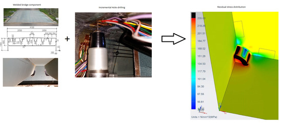
In this paper, an orthotropic steel deck is used to perform residual stress measurements near a welded connection and a semi-destructive measurement technique is used. The incremental hole-drilling method is used to measure residual stresses in the welded steel components. This method is preferred because the measurements can be easily performed at the bridge site without affecting the performance of it. A small hole is drilled in an incremental number of steps and the corresponding strains are measured with strain gauge rosettes on the surface. Residual stresses are calculated with these measured strains and a residual stress distribution into the depth of the material is obtained [
1].
By the evaluation of high residual welding stresses, plastic relaxed strains are introduced near the borehole. This plastic behavior can possibly introduce significant errors in the calculation of the residual stresses since the hole-drilling method only applies when the material behavior remains linear-elastic [
9,
10].
In this paper, the incremental hole-drilling method is simulated using finite element modeling (FEM) with a material model including plasticity. First, uniform in-depth residual stress is simulated and a comparison is made between calibration coefficients specified by the American Society for Testing and Materials ASTM E837-13a and calculated coefficients including the effect of plasticity from the finite element model. Afterwards, non-uniform in-depth residual stresses are studied by evaluating experimental residual stress values of an orthotropic steel deck.
2. Incremental Hole-Drilling Method
Residual stresses introduced by the welding operations for an orthotropic steel deck are evaluated with the incremental hole-drilling method. A small hole is drilled into the test material through the center of a strain gauge rosette [
10]. These strain gauge rosettes are used to measure the relieved surface strains caused by the introduction of a hole that is formed by drilling in a series of small steps. Residual stresses can be calculated with the measured strains and calibration coefficients according to the calculation principles specified in ASTM E837-13a. Reliable measurements are only achieved by limiting the residual stresses to 80% of the material’s yield stress [
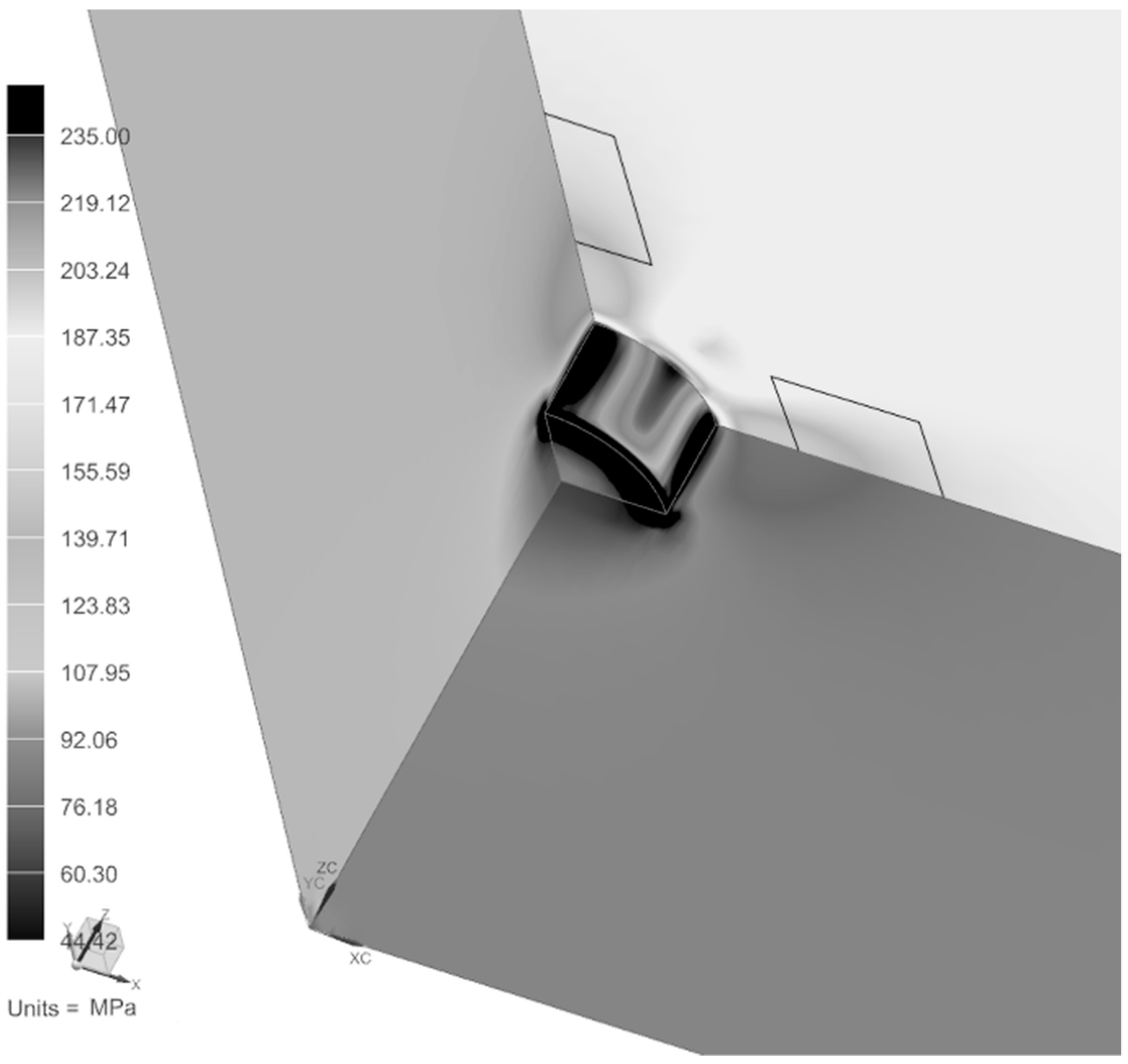
11]. However, the residual stress values can reach the material’s yield stress by drilling of the hole and the elastic limit of the material can be reached. This plastic region is present near the lower circumference of the hole and spreads out towards the strain gauges of the strain gauge rosette by increasing of the hole depth [
10]. The black zones in
Figure 1 indicate this plastic region where a hole drilled up to a depth of 1 mm is simulated for a quarter of a steel plate of quality S235 with 6 mm thickness using a linear-elastic material law. Two strain gauges of a strain gauge rosette are also indicated in the figure.
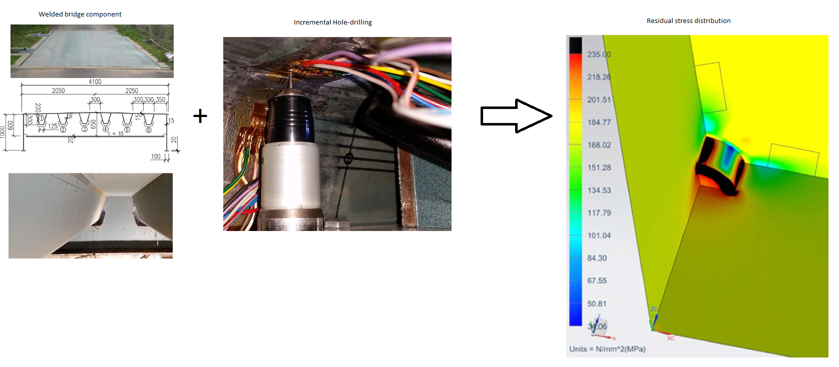
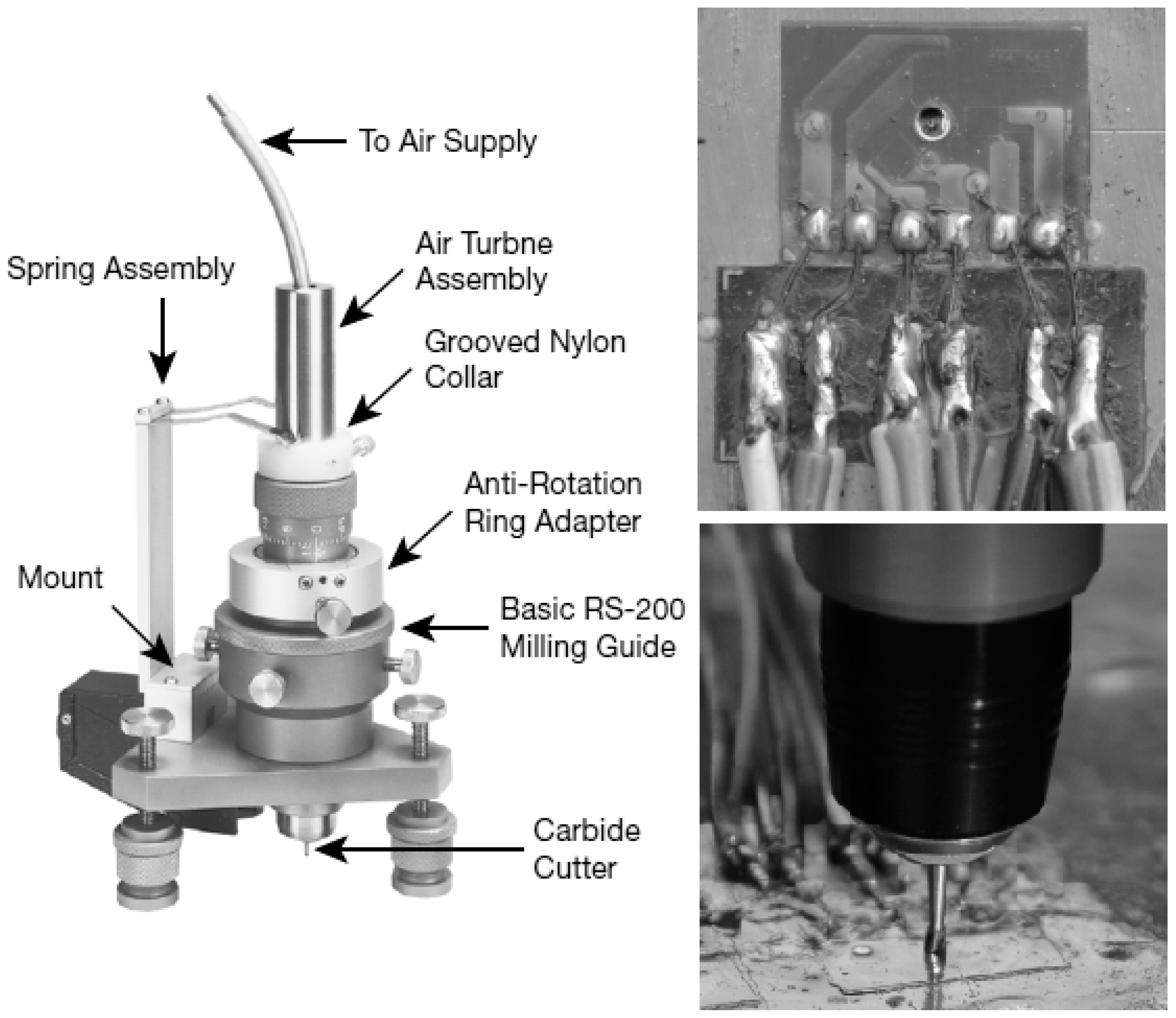
Residual welding stresses introduced by the weld connection of the deck plate with a longitudinal stiffener of an orthotropic steel deck are evaluated with the RS-200 Milling Guide (
Figure 2). For the installation of the strain gauge rosette, a smooth surface is required. However, the surface preparation prior to bonding the strain gauge rosette should not induce significant residual stresses [
10]. The paint layer of the orthotropic steel deck was removed with a grinding tool. After processing the first measurements, it was noticed that the near-surface stresses were very large. By using a grinding disc with less coarse abrasive paper, the near-surface stresses could be reduced. To expose the surface material, it is necessary to drill only through the material of the strain gauge rosette and not trough the material of the test specimen in order to establish the correct zero depth [
10,
12]. In practice, this zero depth is established by very slowly advancing the cutter by 0.02 mm and rotating the drilling machine all the way around. The strains of the strain gauge rosette are recorded and remain constant when the cutter has not yet reached the test surface. When the recorded strains are changing, the cutter has drilled through the material of the strain gauge rosette and reached the surface of the test material. This depth of the cutter indicates the first measurement of the strain gauge rosette. The zero depth is the depth of the cutter before this first measurement.
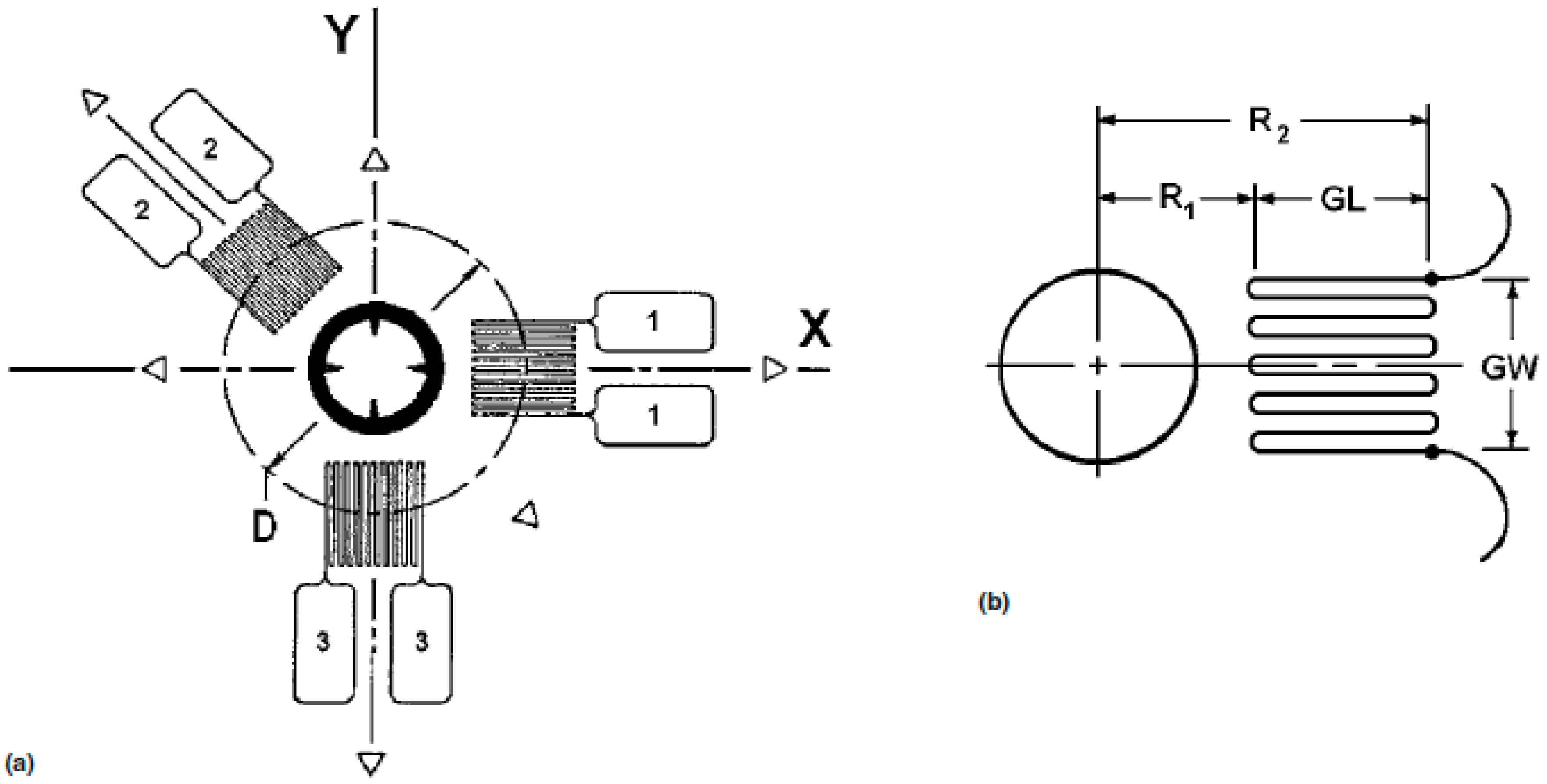
Only one type of strain gauge rosette is used for the measurements on the orthotropic steel deck. Therefore, only this type of strain gauge rosette will be considered in this paper. A strain gauge rosette with the Rendler and Vigness [
13] geometry. Strain gauge rosette type CEA-06-062UL-120 is used for the experimental measurements on the orthotropic steel deck. The geometry is schematically presented in
Figure 3a with a detail of one strain gauge on the rosette in
Figure 3b. The dimensions of the used strain gauge rosette are shown in
Table 1 and it has a hole diameter of 2 mm and a maximum hole-drilling depth of 1 mm [
10].
Bigger strain gauge rosettes can be used to obtain residual stresses more into the depth of the test surface. In this way, the uncertain near-surface residual stresses due to the surface preparations for the strain gauge rosettes can be eliminated. In future research, these bigger strain gauge rosettes can be used to obtain results more into the depth of the material [
11].
3. Three-Dimensional Finite Element Model
Siemens NX11 with solver type Nastran is used to set up a three-dimensional finite element model to determine the plastic relaxed strain readings of the used strain gauge rosette. The grid lines of the strain gauge on the rosette are exactly modeled by element nodes considering the length, spacing, and number of grid lines. The material of the strain gauge rosette is not taken into account. The assumption is made that the measured strains are identical to the relaxed strains [
10,
14]. At both ends of every grid line, the nodal displacements are simulated which are used to determine the radial strains according to following formulae, wherein n equals the total number of grid lines.
The drilling of the incremental holes for the hole-drilling method is simulated by deactivating a layer of elements with an element birth/death feature. For each removed layer, a pressure is applied to the sides of the model containing the hole due to Saint Venant’s principle and the strains are recorded which are used to calculate residual stresses according to ASTM E837-13a. The only interests are the normal x- and y-stresses and therefore only radial strains 1 and 3 (
Figure 3a) are considered to evaluate the residual stresses [
10].
3.1. Geometry, Material Properties, Constraints, and Loading Conditions
A 6 mm thick flat plate is considered to perform the hole-drilling simulation. An increase of the thickness of the plate is studied and there is almost no (less than 1%) effect on the results. Only a quarter of the entire plate has to be considered due to symmetry. The plate is a thick plate according ASTM E837-13a since the thickness of the plate is larger than the mean diameter of the strain gauge rosette. The width of the model is 15 times the hole diameter [
10]. The thickness of the modeled plate is also equal to the thickness of the longitudinal stiffener of the orthotropic steel deck. The steel grade of the orthotropic steel bridge deck is S235. This material is also used for the modeling, resulting in the material parameters specified in
Table 2.
Symmetry constraints are necessary because only a quarter of the plate is considered for the finite element modeling. These constraints are applied on the sides where the hole is situated. The displacements along x- and y-axes along these sides are set to zero. For the bottom surface, the displacement along the z-direction is set to zero [
10].
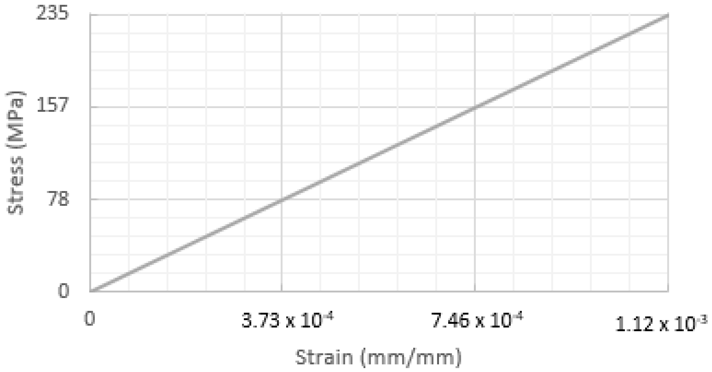
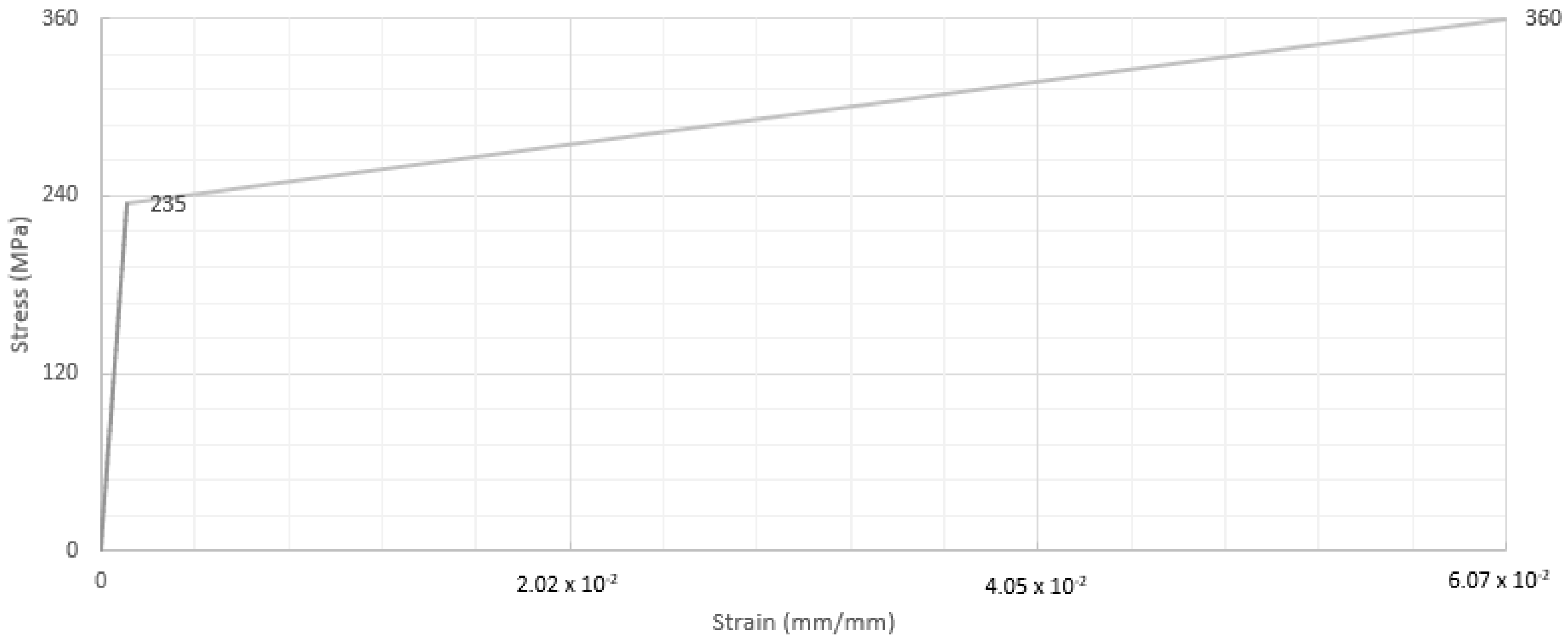
A difference in material behavior is specified with the specification of a different stress–strain curve. A linear stress–strain curve is used for linear-elastic material behavior with the yield stress as an upper limit (
Figure 4). A bilinear stress–strain curve (
Figure 5) is specified when the material behavior is elastic-plastic and an isotropic plasticity hardening model is used [
10].
For the linear-elastic stress–strain behavior, the finite element program follows the same linear curve for the post-critical stresses and strains. For the elastic-plastic stress–strain behavior, the post-critical behavior is determined by the second branch of the curve where it follows the same trend.
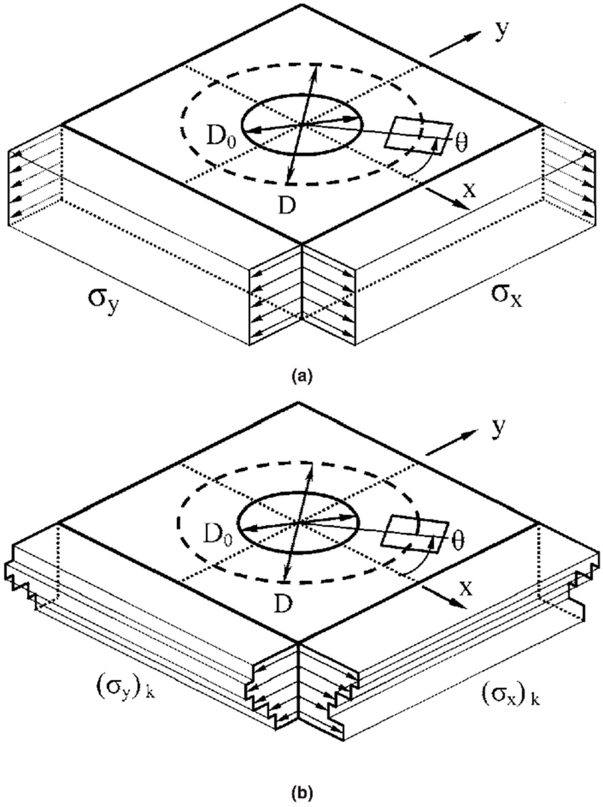
Both uniform (
Figure 6a) and non-uniform (
Figure 6b) in-depth residual stress fields will be evaluated with linear-elastic and elastic-plastic stress–strain behavior. The presence of a residual stress field is simulated by imposing time dependent uniform or non-uniform pressure distributions on the sides not containing the drilled hole. These imposed pressures are assumed to be equal to the principal residual stresses before a hole was drilled [
15]. The drilling of the hole is simulated by a time dependent deactivation of layers in the hole. For each time step that results in a removed layer, a corresponding pressure is applied on the sides at the same height of the hole depth.
Figure 6 gives a representation of the residual stress fields for a drilled hole.
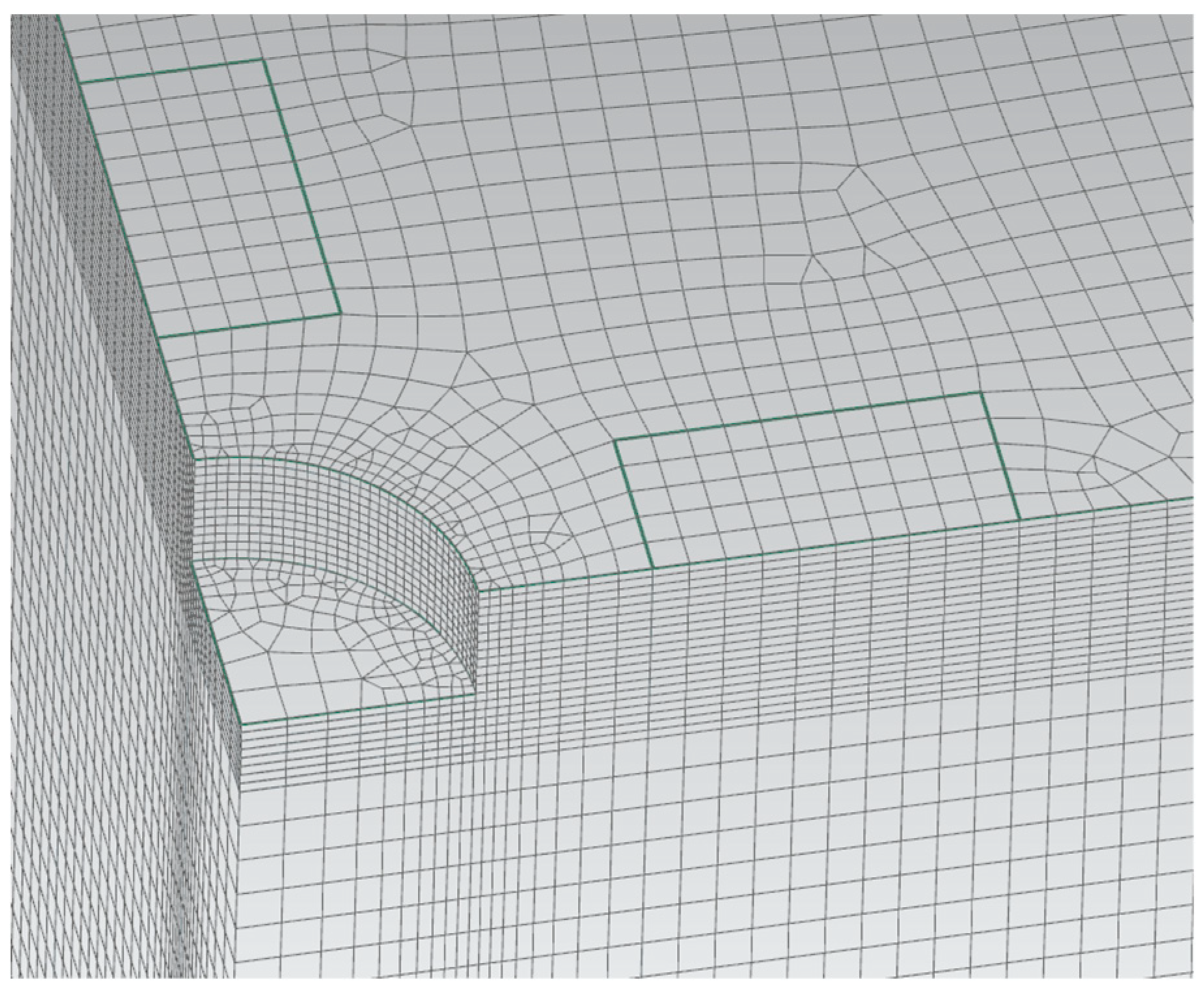
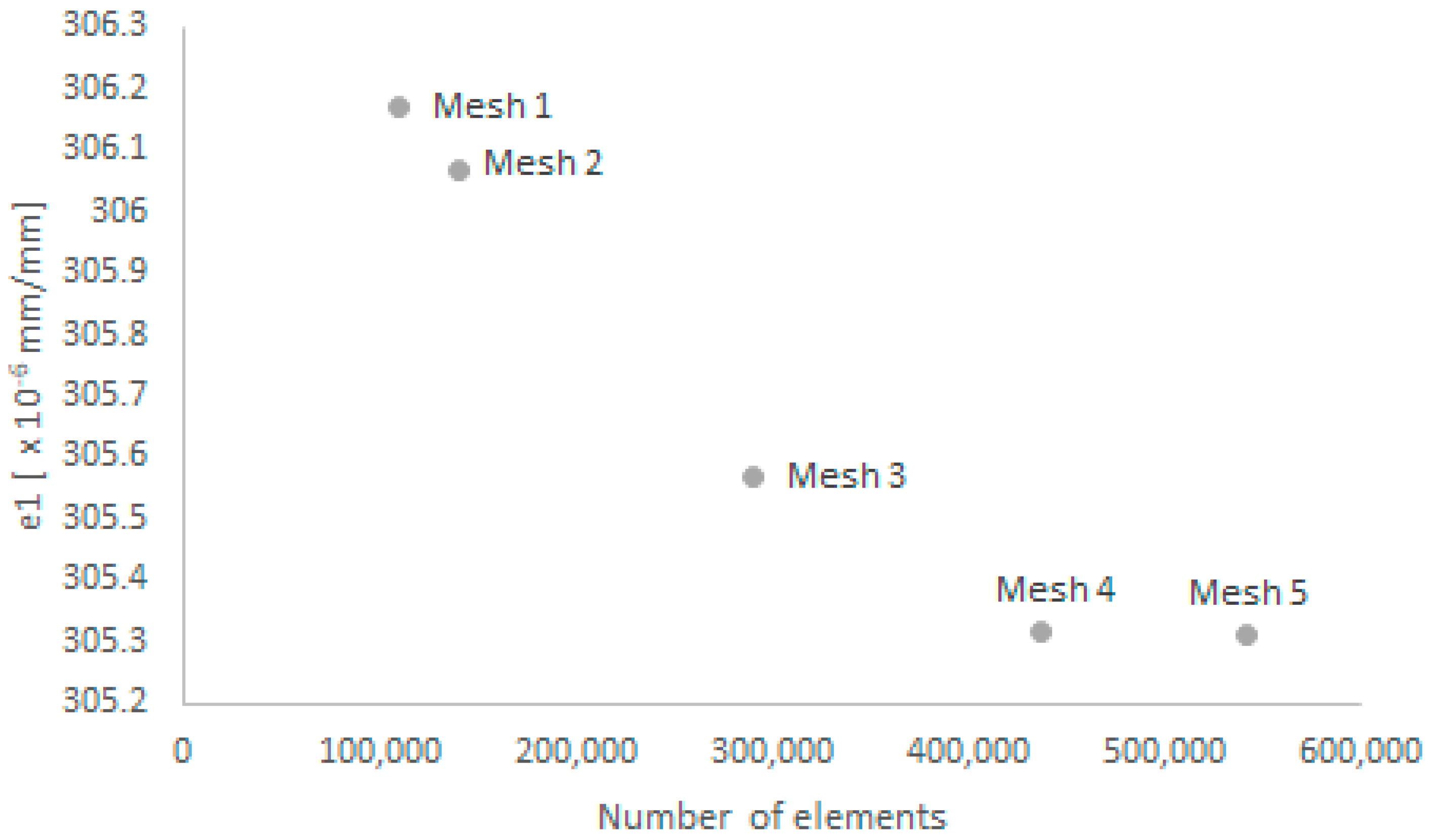
3.2. Mesh Sensitivity Study
The effect of mesh refinement in the area of the drilled hole is studied to examine the element sizes. Therefore, a uniform pressure distribution on the sides not containing the drilled hole is applied along the entire thickness of the plate and a linear-elastic stress–strain behavior is assumed. The strains obtained with this model are compared with the theoretical calculated strains according to ASTM E837-13a. The mesh is further refined until the results of the model are well aligned with the theoretical result. This results in a mesh size of 0.2 mm in a zone of 10 mm around the drilled hole. The rest of the model has a mesh size of 0.5 mm. The mesh size near the drilled hole is smaller since a higher precision is required for an accurate evaluation of the strains on the strain gauge rosette. Outside the drilled hole region and further away from the strain gauges, a less high precision is required resulting in a shorter calculation time. There are 436,410 three-dimensional hexagonal CHEXA-elements with eight nodes present in the entire model when there is no material removed by the drilling procedure. The depth increments where material has to be removed during the hole-drilling process are meshed separately. This mesh will be used as a reference for all 3D models used in this paper. The finite element model for drilling the hole is shown in
Figure 7.
When the mesh is further refined, the calculation time increases drastically and the precision stays almost the same. The procedure for the mesh refinement is shown in
Figure 8. The mesh refinement for radial strain 1 is displayed which is the radial strain in the x-direction and mesh 4 is the mesh used for further calculations.
3.3. Residual Stress Calculation
For uniform in-depth residual stress distributions, the principal residual stresses
σx and
σy can be calculated from the calibration coefficients a and b, the measured relaxed strains
ϵ1 and
ϵ3, Poisson’s ratio ν, and the Young’s modulus E of the material [
11]. The following relationships apply:
The calibration coefficients are dependent on the hole depth, type of strain gauge rosettes, and hole diameter of the drilled hole. A known uniform stress distribution is applied on the sides where the hole is not situated and the relaxed strains are evaluated to calculate these calibration coefficients [
9,
10].
For non-uniform residual stress distributions, the relation between residual stresses and relaxed strains is more difficult compared to uniform distributions. The standard errors in the combination strain vectors should also be considered to determine the principal residual stresses. For non-uniform residual stress fields, the calculated relaxed strains of the 3D model will be compared with the theoretical determined relaxed strains according ASTM E837-13a of an orthotropic bridge deck. These strains are used to determine a residual stress distribution of the orthotropic bridge deck.
4. Uniform In-Depth Residual Stress Field
A uniform in-depth residual stress field is simulated by applying known uniform pressure on the sides of the model. The drilling of the hole happens in different time steps and for each removed layer, a pressure of the same height on the side is applied. First, linear-elastic material behavior will be applied for the determination of the calibration coefficients. Then, simplified material plasticity is applied and a comparison is made between the results of the two different material laws.
4.1. Linear-Elastic Material Properties
First, the hole-drilling process is numerically calibrated with a test piece where a uniform in-depth residual stress field of 50 MPa is applied on and the calibration coefficients are determined. The uniform residual stress field is divided into equi-biaxial (σ
x = σ
y = 50 MPa) and deviatoric (σ
x = −σ
y = 50 MPa) residual stress fields and a linear-elastic material law is considered. Two 3D models with linear-elastic material behavior are evaluated. A known equi-biaxial stress field is applied on the first model while the second model is evaluated by applying a deviatoric stress field. The model with equi-biaxial residual stress field is used to determine calibration coefficient a. A deviatoric residual stress field gives calibration coefficient b. Ten depth-step increments of 0.1 mm are evaluated for both models until a final hole depth of 1 mm is reached. The calibration coefficients are calculated by evaluating the relaxed strains for each depth-step [
10]. Uniform in-depth residual stress fields of 100 MPa and 150 MPa were also considered which resulted in the same calibration coefficients. In
Table 3 the calculated calibration coefficients are shown. The coefficients for elastic-plastic material behavior are also already mentioned.
The calibration coefficients from the finite element modeling with linear-elastic material behavior should equal the coefficients specified in ASTM. However, the coefficients calculated with the 3D model are on average 4% smaller compared with the ones from ASTM. By increasing the hole depth, the difference also increases because the distance to the strain gauge rosette on the surface increases. There is less contribution of the relaxed strain at the deeper hole depth increments because the distance to the surface of the strain gauge rosette increases. Geometric variables such as the hole diameter, plate thickness, and drilling depth have an influence on the determination of the calibration coefficients. Measurement errors of strain, hole depth, and geometry cause a difference between the calibration coefficients determined with finite element modeling and specified in ASTM. Research conducted by Aoh and Wei [
16] shows that calibration coefficient a becomes ill conditioned faster than calibration coefficient b and this can also can be noticed in
Table 3.
There is also a comparison made with coefficients from other studies [
16] and similar error rates and trends are observed in the experimental calibration. Therefore it is concluded that the calibration coefficients from the three-dimensional finite element modeling are in agreement with the conventional coefficients of the incremental hole-drilling method specified in ASTM. This finite element model is used to model the incremental hole drilling for the determination of residual stresses in an orthotropic bridge deck [
10].
4.2. Elastic-Plastic Material Properties
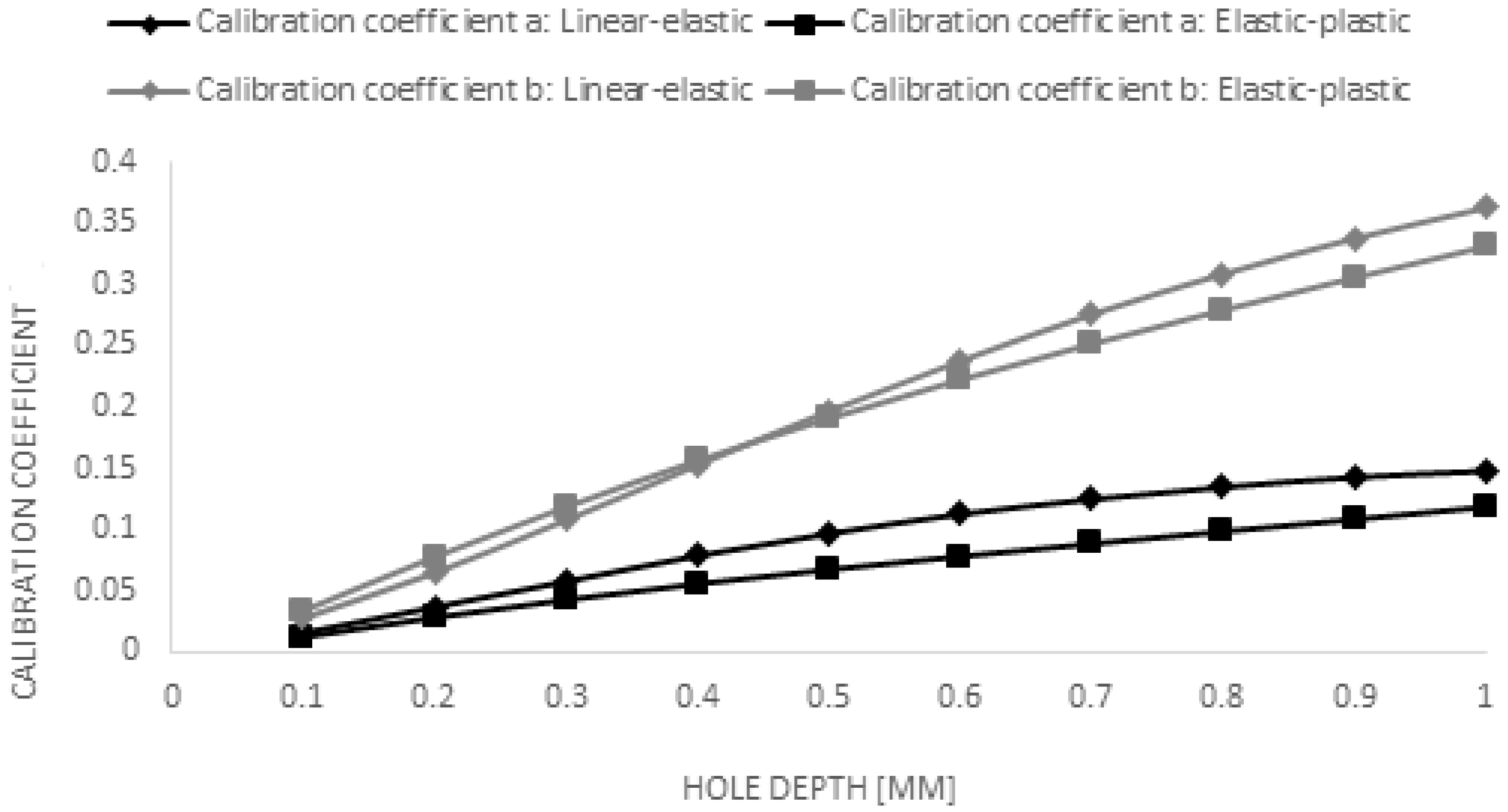
The calibration coefficients determined with linear-elastic and elastic-plastic finite element models are compared and this is shown in
Figure 9. Elastic-plastic material behavior coefficients are smaller, only for the first hole depth is calibration coefficient b larger. The difference between the two material behaviors also increases by an increasing hole depth. A smaller calibration coefficient means that the residual strains and their corresponding stresses are lower than the theoretical ones. Therefore, linear-elastic material behavior gives an overestimation of the residual stresses. The effect of plasticity is more pronounced for deviatoric residual stress fields [
10].
5. Non-Uniform In-Depth Residual Stress Field of the Orthotropic Bridge Deck
A non-uniform in-depth residual stress field of the orthotropic steel deck is simulated by applying a non-uniform pressure on the sides of the model not containing the drilled hole. The non-uniform residual stress field is obtained by hole-drilling measurements. The results of the finite element modeling will be compared with the experimental results from the hole-drilling measurements.
5.1. Experimental Hole-Drilling Measurements
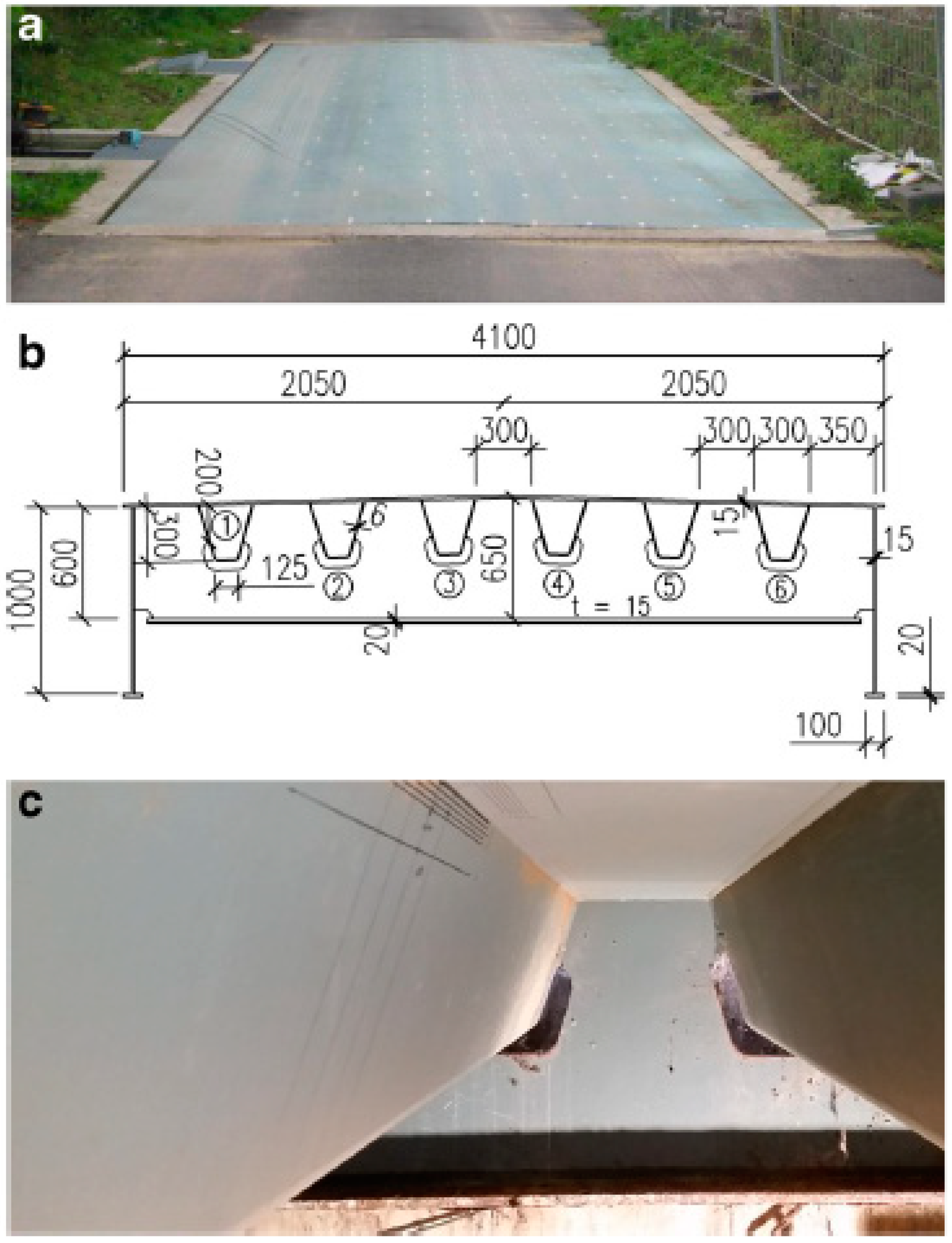
Experimental residual stress measurements on an orthotropic steel deck are performed with the incremental hole-drilling procedure according the ASTM standard. The full scale test specimen used for the measurements is shown in
Figure 10 [
17]. The longitudinal stiffeners are welded to the bridge deck plate with twin wire submerged arc welding. The welding can only be executed from the outside of the stiffener since the inside cannot be reached with a welding torch. The parameters of the welding procedure are provided by the manufacturer. The diameter of the electrodes is 2 mm while the extension of one electrode is 30 mm. The welding is executed with a current op 780 A and a voltage of 29 V. The advancing speed of the welding torches is 950 mm per minute. The welding current flows from the electrode to the base metal.
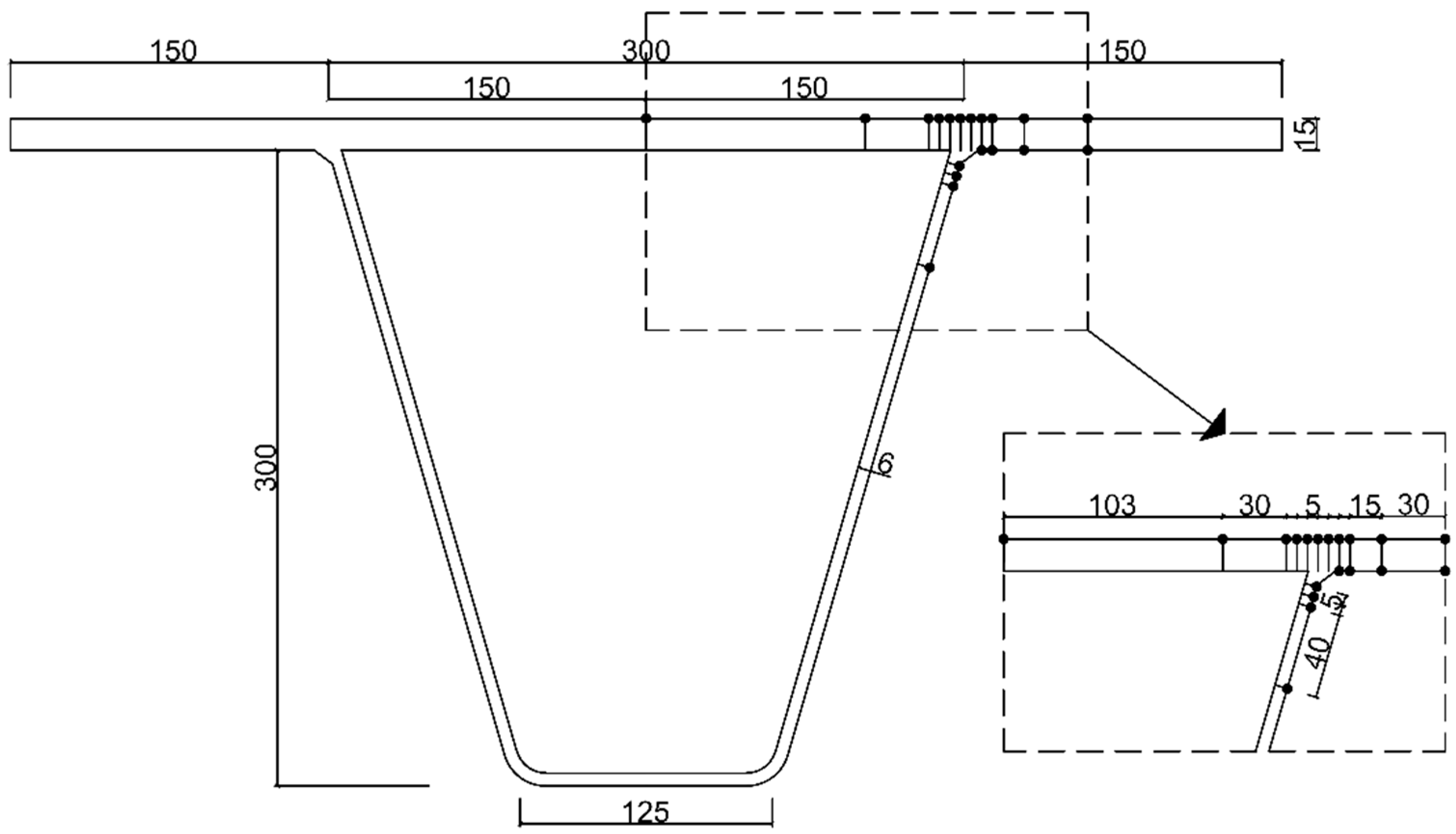
Locations on the top and bottom of the deck plate and on the longitudinal stiffener are evaluated. Strains are measured at incremental depths of 0.05 mm until a final hole depth of 1 mm is reached. A single representative value for the residual stress is selected for each strain gauge rosette in the residual stress distribution into the depth of that particular strain gauge rosette. The near surface stresses are affected by the grinding disc which is used to prepare the surface for the installation of the strain gauge rosette. The residual stress at the final hole depth of 1 mm is considered to minimize the impact of the surface preparation on the residual stress value. A residual stress distribution for the longitudinal and transverse directions can be established in relation to the distance to the weld. The locations of the different strain gauge rosettes are displayed in
Figure 11.
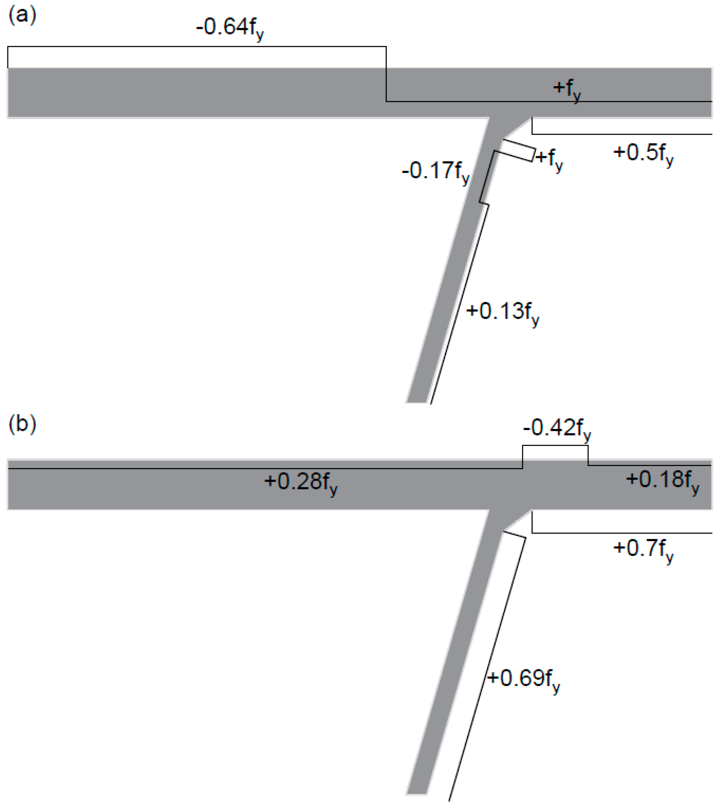
A residual stress value is assigned to each measured strain gauge rosette for the transverse and longitudinal directions. This residual stress value is the calculated stress at the final hole depth according the calculation principles of the ASTM standard for both directions. Since the values of the residual stresses vary for neighboring strain gauge rosettes, a distinction is made between compressive and tensile residual stress values. The measured locations are grouped in compressive and tensile zones. The residual stress values assigned to these zones are calculated by averaging the residual stresses of the strain gauge rosettes present in the considered zone. Positive values indicate tensile residual stresses while negative values indicate compressive stresses. In the longitudinal direction, there is a tensile and a compressive residual stress zone present on top of the deck plate. The tensile zone has a value of 64% of the yield strength (f
y) while the compressive zone reaches the yield strength. For the bottom of the deck plate, there is a tensile residual stress zone (0.5 × f
y) present in the longitudinal direction. On the stiffener, there is a small tensile yield stress zone present near the weld which is followed by a compressive zone (0.17 × f
y) and a tensile zone (0.13 × f
y). For the transverse direction, two tensile zones and a compressive zone are recognized on the top of the deck plate. In between the two welded webs of the stiffener, an average tensile residual stress of 67 MPa exists. Near the weld location on the deck plate, there is a compressive zone with an average residual stress equal to 0.42 × f
y. Another tensile residual stress zone exists at the right-hand side of the weld region on the deck plate. On the bottom side of the deck plate, an average tensile residual stress equal to 70% of the yield strength exists. For the longitudinal stiffener, there is a tensile residual stress zone present near the weld. These general residual stress distributions obtained with the experimental results are shown in
Figure 12.
Residual stresses are self-equilibrating since they remain within the material even after the initial cause of the stresses (welding) is removed. Therefore, the sum of all stresses in a local area creates zero resultant force and zero momentum. More hole-drilling measurements along the entire steel deck are necessary to verify to self-equilibrium. However, the residual stress distribution on top of the deck plate for the transverse direction indicates a good balance.
5.2. Finite Element Modeling Results
The hole-drilling procedure of the experimental setup for the orthotropic steel deck is simulated with finite element modeling. The hole is drilled in 20 depth steps of 0.05 mm until the final hole depth of 1 mm is reached. For each step, material is removed and stress is relieved. To compensate for this material removal, a corresponding pressure is applied at the sides of the model. In this way, the external force balance of stresses remains in equilibrium. The applied pressures correspond with the experimentally-obtained results and the residual stresses can be calculated for each drilling depth. This allows the comparison of the results obtained with experimental measurements and finite element modeling.
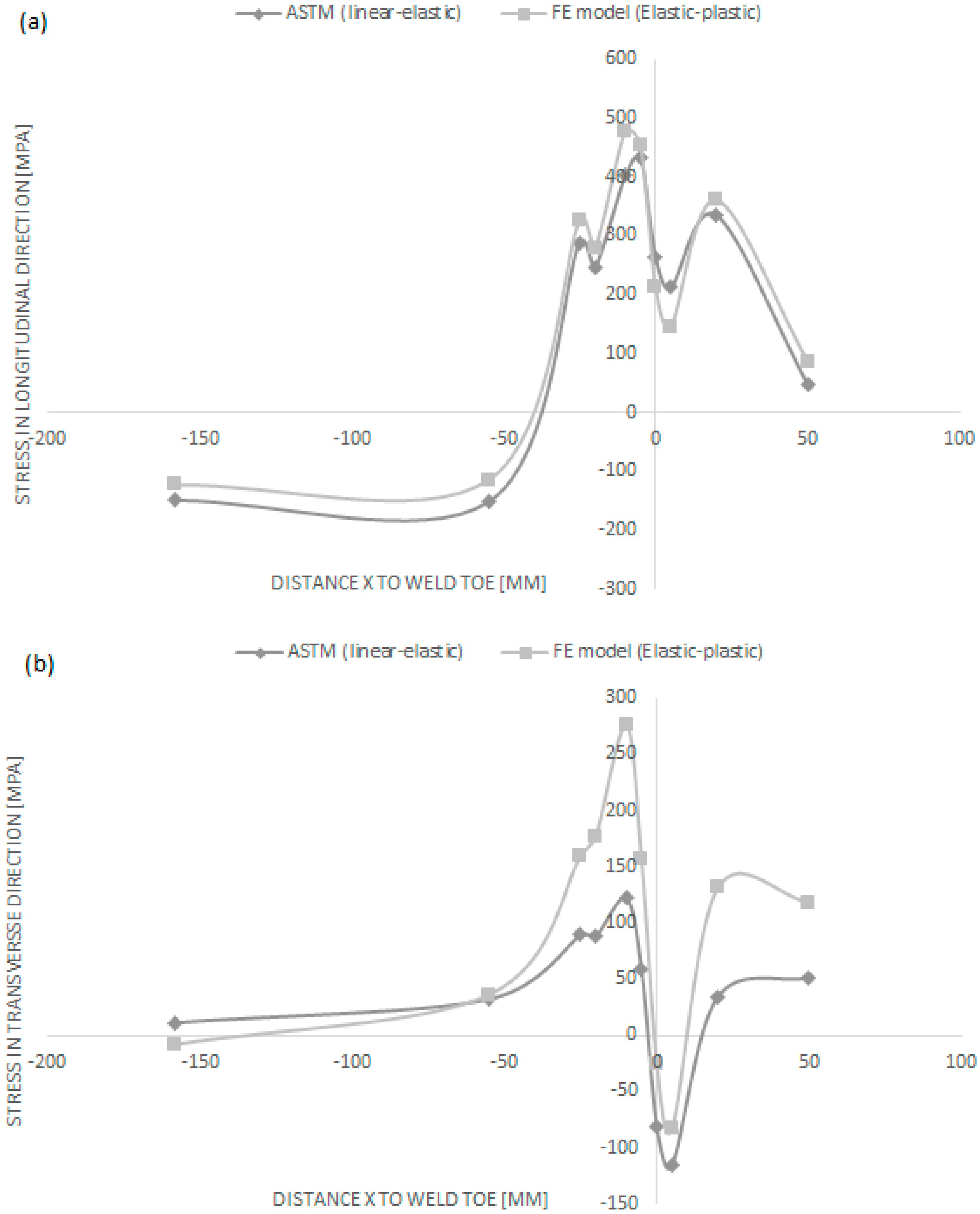
5.2.1. Top Side Deck Plate
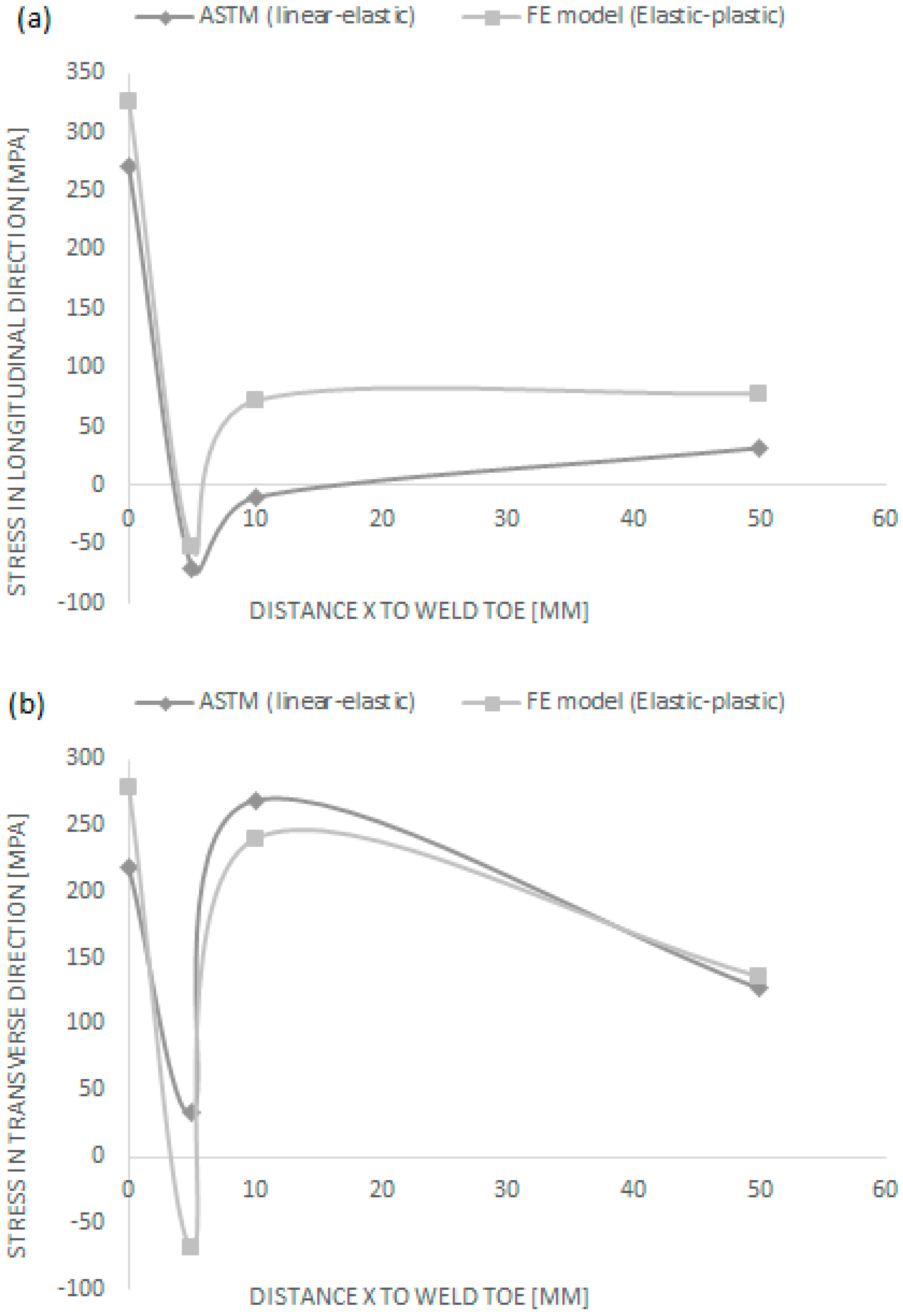
A total of 11 strain gauge rosettes are investigated on the top side of the deck plate. The measured residual stresses for each of these strain gauge rosettes at 20 incremental depths of 0.05 mm are applied to the 3D model on the boundaries not containing the hole and the hole-drilling procedure is simulated. The incremental strains obtained with the 3D model are used to calculate the residual stresses. For each strain gauge rosette, a representative residual stress value at the final hole depth of 1 mm is used to make a residual stress distribution in function of distance to the weld toe. The experimentally-determined residual stress distribution is compared with the measured residual stress distribution from the finite element model for both the transverse and longitudinal directions. This comparison is shown in
Figure 13. The horizontal axis gives the distance to the weld toe, the origin corresponds to the weld toe while positive distances are at the right-hand side of the weld toe and negative distances at the left-hand side.
The residual stress values obtained with elastic-plastic analysis result in higher tensile and lower compressive residual stresses compared to the expected ones from the experimental measurements according the ASTM standard. However, the general trend of the stresses in relation to the distance to the weld toe remains the same.
5.2.2. Bottom Side Deck Plate
On the bottom side of the deck plate, a total of 4 strain gauge rosettes are evaluated. In function of distance to the weld toe, the experimentally-expected residual stress distribution and the residual stress distribution calculated with the finite element model with elastic-plastic material behavior are shown in
Figure 14.
Again, the residual stress distribution from the 3D finite element model (FEM) shows a similar trend compared to the experimental measurements according ASTM. For the bottom side of the deck plate there are only tensile residual stresses which are higher for the results from the finite element modeling.
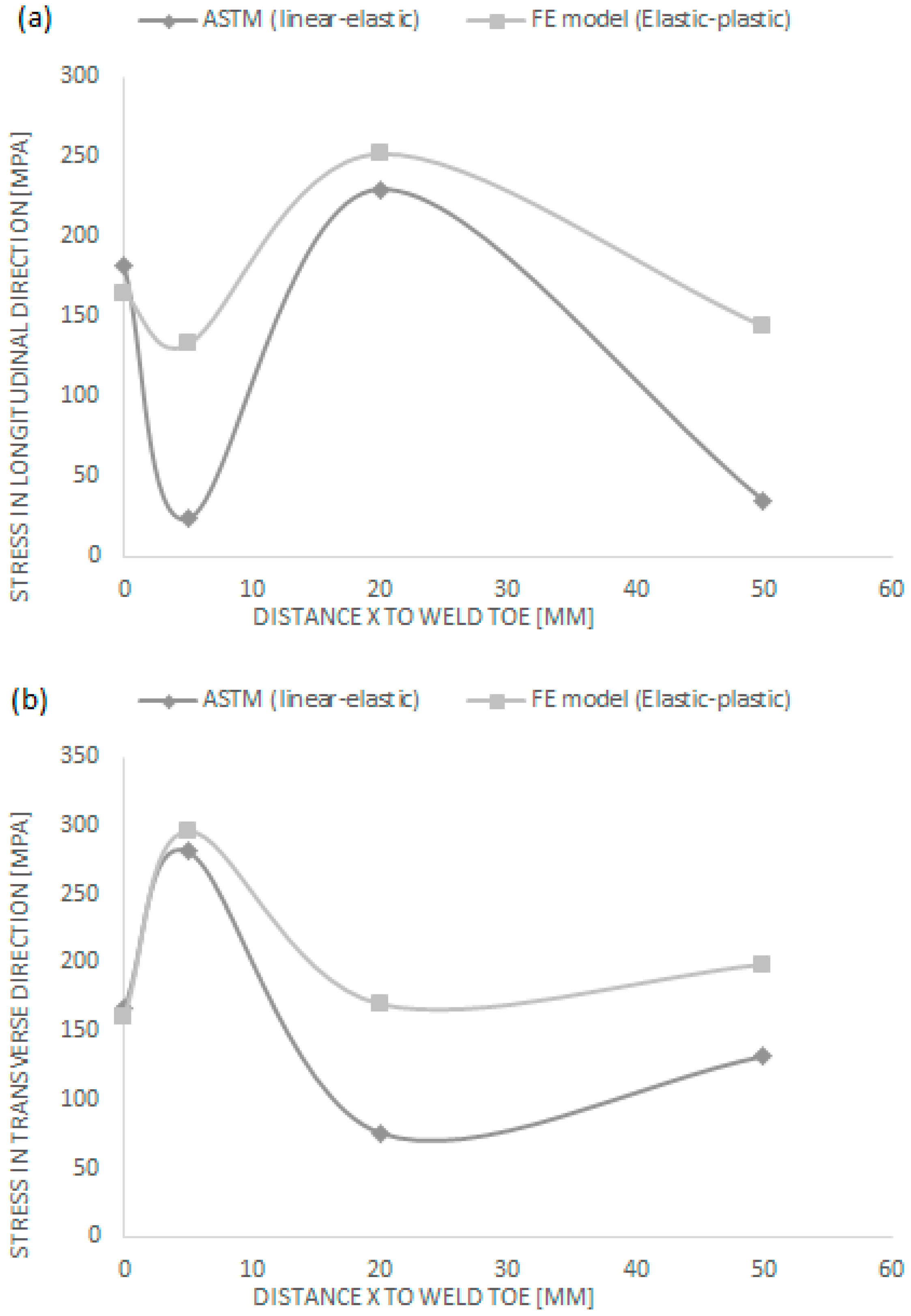
5.2.3. Longitudinal Stiffener
Finally, the 4 strain gauge rosettes located on the longitudinal stiffener are evaluated with the finite element model. The results are shown in
Figure 15.
The same trends are again observed. The residual stress distribution from the 3D model shows higher tensile and lower compressive residual stresses compared with the results from ASTM. The course of the residual stresses in function of the distance to the weld toe remain similar for the experimental and numerical results from the finite element modeling.
5.3. Residual Stress Distribution of the Orthotropic Steel Deck
The residual stresses from the experimental measurements are implemented in a finite element model and the results are shown in
Section 5.2. These residual stress results are more representative since the finite element model makes use of an elastic-plastic material model which is more realistic than the elastic behavior of the experimental setup. A general residual stress distribution is established in relation to the distance to the weld which can be compared with
Figure 12. Also here, a distinction is made between compressive and tensile residual stress zones and both the longitudinal and transverse direction are considered. The residual stress values assigned to these zones are calculated by averaging the residual stresses of the strain gauge rosettes present in the considered zone. This residual stress distribution is shown in
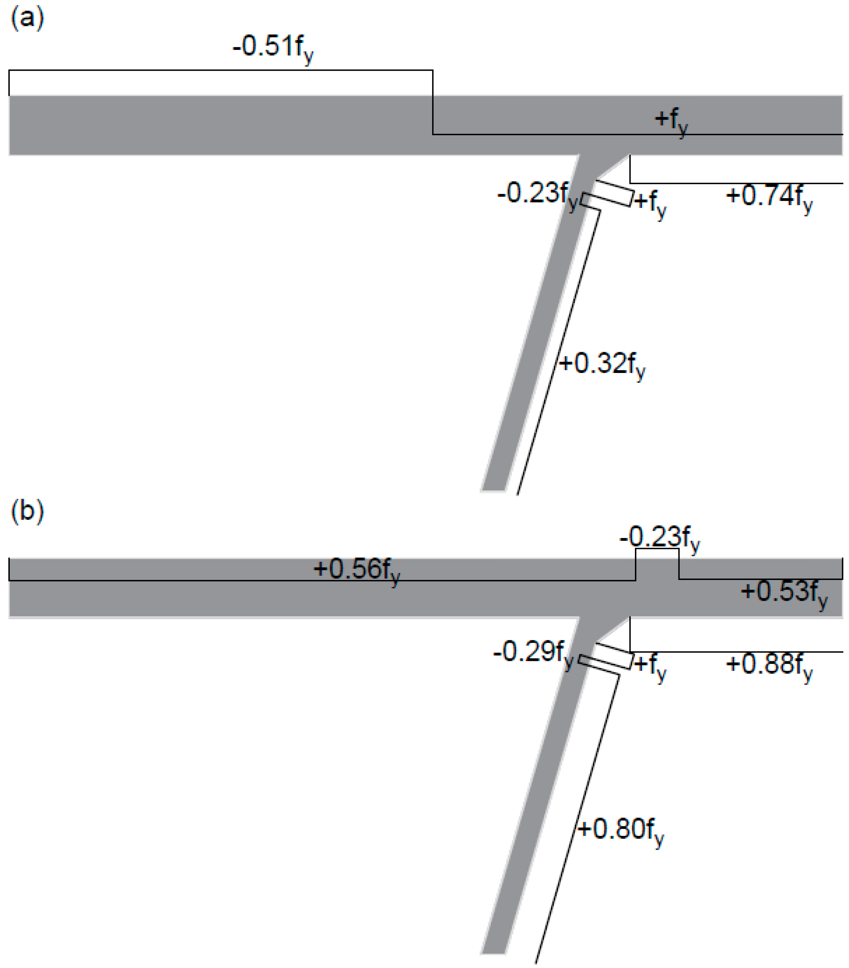
Figure 16a for the longitudinal direction and
Figure 16b for the transverse direction.
In the longitudinal direction, there is a tensile and a compressive residual stress zone present on top of the deck plate. The tensile zone has a value of 51% of the yield strength (fy) while the compressive zone reaches the yield strength. For the bottom of the deck plate, there is a tensile residual stress zone of 0.74 × fy present in the longitudinal direction. On the stiffener, there is a small tensile yield stress zone present near the weld which is followed by a compressive and a tensile zone. For the transverse direction, two tensile zones and a compressive zone are recognized on the top of the deck plate. In between the two welded webs of the stiffener, an average tensile residual stress of 133 MPa exists, this corresponds to 56% of the yield strength. Near the weld location on the deck plate, there is a compressive zone with an average residual stress equal to 0.23 × fy. Another tensile residual stress zone with an average value of 53% of the yield strength exists at the right-hand side of the weld region on the deck plate. On the bottom side of the deck plate, an average tensile residual stress equal to 0.88 × fy exists. For the longitudinal stiffener, there is a small tensile yield stress zone present near the weld which is followed by very small compressive residual stresses, close to zero. Further away from the weld, there is a tensile residual stress zone of 80% of the yield strength present.
When the results of the finite element modeling (
Figure 16) are compared with the residual stresses from the experimental measurements (
Figure 12), a general residual stress distribution of the orthotropic steel deck can be established. The FEM results are more representative since it makes use of a more realistic material model. First the results of the longitudinal direction are discussed. There is a compressive zone present between the two welded webs of the stiffener on top of the deck plate. This compressive zone is equal to half of the material’s yield strength according to the FEM results. This is 10% smaller compared to the results from the experimental setup. Near the weld region on top of the deck plate, there are tensile yield residual stresses present. On the bottom side of the deck plate, there is a tensile zone of 74% of the yield strength present for the results from the finite element modeling. This is 24% larger than the value from the experimental results. For the stiffener, there is a small tensile yield zone present near the weld which is followed by a small compressive zone of 23% of the yield strength. This compressive zone is smaller in size compared to the one from the experimental measurements and the value is 6% larger. Finally, there exists a tensile zone along the rest of the stiffener with a value of 32% of the material’s yield strength. This is 19% larger compared to the experimental data. For the longitudinal direction it can be concluded that similar residual stress zones are present for both the FEM and experimental results. The compressive residual stresses remain the same within a margin of approximately 10%. The tensile residual stresses are in general 20% larger for the FEM results.
In the transverse direction, there are three different zones that can be recognized on top of the deck plate. A tensile zone of 56% of the yield strength in between the welded webs of the stiffener followed by a compressive zone of 23% of the yield strength near the welding region and again a tensile zone of 53% of the material’s yield strength. The tensile residual stresses are respectively 28% and 35% larger for the FEM results. The compressive residual stress values are 19% smaller. On the bottom side of the deck plate there is a tensile residual stress zone with a value of 88% of the yield strength. This results in residual stresses that are 18% larger compared to the experimental results. For the longitudinal stiffener, a totally different residual stress behavior is noticed for the FEM results. The results from the experimental data show tensile residual stresses equal to 69% of the yield strength along the entire stiffener. However, the FEM results show a tensile yield zone near the weld followed by a small compressive zone where the residual stress is close to zero and again a tensile stress zone of 80% of the yield strength. For the transverse direction, similar residual stress zones are recognized for the deck plate. The longitudinal stiffener shows a different residual stress behavior. In general, it can be concluded that the tensile residual stress values are larger for the FEM results compared to the experimental results and the compressive residual stresses are smaller.
The finite element modeling of the hole-drilling method for the orthotropic steel deck gives the effect of the residual stresses including a more realistic material model. This results in larger tensile residual stresses and lower compressive stresses. Therefore, it can be concluded that the experimental results from the hole-drilling method calculated according the ASTM standard underestimate the tensile residual stresses and overestimate the compressive residual stresses. Since larger tensile residual stresses are more harmful for the fatigue of a welded bridge component, it is better to include the real material properties with elastic-plastic behavior. In this case, the verification of the hole-drilling results with finite element modeling is very valuable.
6. Conclusions
The incremental hole-drilling method can be used to evaluate high residual welding stresses for welded bridge constructions. This method only applies when material behavior is linear-elastic and therefore, the effect of including the real material properties with elastic-plastic behavior on residual stresses calculated according ASTM E837-13a is studied with three-dimensional finite element modeling. The hole-drilling procedure is simulated with a calculation software. First, a linear-elastic analysis is executed to determine calibration coefficients similar to the ones specified in ASTM E837-13a for uniform in-depth residual stresses. For a uniform in-depth residual stress field, a superposition is made of equi-biaxial and deviatoric residual stress fields applied on the sides of the model. Then, the effect of plasticity on the uniform in-depth residual stresses is determined by applying an elastic-plastic material law to the same 3D model. It is concluded that the residual stresses obtained under the assumption that the material behavior is linear-elastic are an overestimation. The plasticity introduces relaxation of the material and by ignoring this, the residual stresses will be overestimated by specifying linear-elastic material behavior.
The effect of the elastic-plastic material behavior for non-uniform in-depth residual stresses is also studied by comparing experimentally-determined radial strains with calculated strains from elastic-plastic analysis of an orthotropic steel deck. Similar behavior of the residual stresses were noticed. However, the residual stresses obtained with the elastic-plastic analysis of the finite element model are larger for tensile and smaller for compressive residual stresses.
An accurate fatigue design including the residual welding stresses is very important since one of the most important failure modes for steel bridges with welded structural members is fatigue failure. The finite element modeling showed larger tensile residual stresses compared with the analysis according ASTM. Larger tensile residual stresses accelerate stress corrosion cracking leading to an earlier fatigue failure of the component. Therefore, it is very important to take these larger tensile residual stresses into account for the fatigue design of the welded component.
The experimentally-determined residual stress values of the orthotropic steel deck according the ASTM standard are based on linear-elastic material behavior. The finite element modeling showed that including an elastic-plastic material model resulted in larger tensile and smaller compressive residual stresses. This behavior is more disadvantageous since it leads to premature fatigue cracking. Therefore, it is very valuable to verify the experimental hole-drilling results with finite element modeling including the material’s elastic-plastic behavior.
Author Contributions
Conceptualization: E.V.P., W.N., and H.D.B.; Data curation: E.V.P.; Formal analysis: E.V.P.; Investigation: E.V.P., W.N., and H.D.B.; Methodology: E.V.P. and W.N.; Project administration: E.V.P., K.S., and H.D.B.; Resources: K.S. and H.D.B.; Software: E.V.P. and W.N.; Supervision: K.S. and H.D.B.; Validation: E.V.P., Z.U.-A., and W.N.; Visualization: E.V.P. and W.N.; Writing—original draft: E.V.P. and H.D.B.; Writing—review and editing: E.V.P., Z.U.-A., and H.D.B.
Funding
This research received no external funding.
Conflicts of Interest
The authors declare no conflict of interest.
References
- Schajer, G.S. Practical Residual Stress Measurement Methods; John Wiley & Sons Ltd.: Chichester, UK, 2013. [Google Scholar]
- Huang, C.C.; Pan, Y.C.; Chuang, T.H. Effects of Post-Weld Heat Treatments on the Residual Stress and Mechanical properties of Electron Beal Welded SAE 4130 Steel Plates. J. Mater. Eng. Perform. 1997, 6, 61–68. [Google Scholar] [CrossRef]
- Ganguly, S.; Sule, J.; Yakubu, M.Y. Stress Engineering of Multi-pass Welds of Structural Steel to Enhance Structural Integrity. J. Mater. Eng. Perform. 2016, 25, 3238–3244. [Google Scholar] [CrossRef]
- Zhao, Z.; Haldar, A.; Breen, F.L. Fatigue-Reliability Evaluation of Steel Bridges. J. Struct. Eng. 1994, 120, 1608–1623. [Google Scholar] [CrossRef]
- Sonsino, C.M. Effect of residual stresses on the fatigue behavior of welded joints depending on loading conditions and weld geometry. Int. J. Fatigue 2009, 31, 88–101. [Google Scholar] [CrossRef]
- Prevéy, P.S.; Mason, P.W.; Hornbach, D.J.; Molkenthin, J.P. Effect of Prior Machining Deformation on the Development of Tensile Residual Stresses in Weld Fabricated Nuclear Components. J. Mater. Eng. Perform. 1996, 5, 51–56. [Google Scholar] [CrossRef]
- Zinn, W.; Scholtes, B. Mechanical Surface Treatments of Lightweight Materials—Effects on Fatigue Strength and Near-Surface Microstructures. J. Mater. Eng. Perform. 1999, 8, 145–151. [Google Scholar] [CrossRef]
- Rossini, N.; Dassisti, M.; Benyounis, K.; Olabi, A. Methods of measuring residual stresses in components. Mater. Des. 2012, 35, 572–588. [Google Scholar] [CrossRef]
- Beghini, M.; Bertini, L.; Santus, C. A procedure for evaluating high residual stresses using the blind hole drilling method, including the effect of plasticity. J. Strain Anal. Eng. Des. 2010, 45, 301–318. [Google Scholar] [CrossRef]
- Van Puymbroeck, E.; Nagy, W.; De Backer, H. Effect of Plasticity on Residual Stresses Obtained by the Incremental Hole-drilling Method with 3D FEM Modelling. Mater. Res. Proc. 2016, 2, 235–240. [Google Scholar]
- ASTM International. Standard Test Method for Determining Residual Stresses by the Hole-Drilling Strain-Gage Method; ASTM E837-13a; ASTM International: West Conshohocken, PA, USA, 2015. [Google Scholar]
- Vishay Measurements Group. Model RS-200 Milling Guide Instruction Manual Version 2.0; Micro-Measurements: Malvern, PA, USA, 2011. [Google Scholar]
- Rendler, N.J.; Vigness, I. Hole-drilling strain gage method of measuring residual stresses. Exp. Mech. 1966, 6, 577–586. [Google Scholar] [CrossRef]
- Nau, A.; Scholtes, B. Evaluation of the High-Speed Drilling Technique for the Incremental Hole-Drilling Method. Exp. Mech. 2013, 53, 531–542. [Google Scholar] [CrossRef]
- Beghini, L.; Bertini, L. Recent Advances in the Hole Drilling Method for Residual Stress Measurement. J. Mater. Eng. Perform. 1998, 7, 163–172. [Google Scholar] [CrossRef]
- Aoh, J.N.; Wei, C.S. On the Improvement of Calibration Coefficients for Hole-Drilling Integral Method: Part I-Analysis of Calibration Coefficients Obtained by a 3-D FEM Model. J. Eng. Mater. Technol. 2002, 124, 250–258. [Google Scholar] [CrossRef]
- Nagy, W.; Van Puymbroeck, E.; Schotte, K.; Van Bogaert, P.; De Backer, H. Measuring Residual Stresses in Orthotropic Steel Decks Using the Incremental Hole-Drilling Technique. Exp. Tech. 2017, 41, 215–226. [Google Scholar] [CrossRef]
Figure 1.
Plastic zone introduced by hole drilling.
Figure 1.
Plastic zone introduced by hole drilling.
Figure 2.
RS-200 Milling Guide (left) and hole-drilled strain gauge rosette (right).
Figure 2.
RS-200 Milling Guide (left) and hole-drilled strain gauge rosette (right).
Figure 3.
Schematic geometry of a strain gauge rosette (a) and detail of one strain gauge (b).
Figure 3.
Schematic geometry of a strain gauge rosette (a) and detail of one strain gauge (b).
Figure 4.
Linear-elastic stress–strain behavior.
Figure 4.
Linear-elastic stress–strain behavior.
Figure 5.
Elastic-plastic stress–strain behavior.
Figure 5.
Elastic-plastic stress–strain behavior.
Figure 6.
(a) Uniform in-depth and (b) non-uniform in-depth residual stress field.
Figure 6.
(a) Uniform in-depth and (b) non-uniform in-depth residual stress field.
Figure 7.
Finite element model with drilled hole.
Figure 7.
Finite element model with drilled hole.
Figure 8.
Mesh sensitivity study.
Figure 8.
Mesh sensitivity study.
Figure 9.
Comparison between linear-elastic and elastic-plastic material behavior from 3D models.
Figure 9.
Comparison between linear-elastic and elastic-plastic material behavior from 3D models.
Figure 10.
Full scale test specimen (a) top view; (b) cross section; (c) bottom view between two longitudinal stiffeners.
Figure 10.
Full scale test specimen (a) top view; (b) cross section; (c) bottom view between two longitudinal stiffeners.
Figure 11.
Locations of measured strain gauge rosettes (dimensions in mm).
Figure 11.
Locations of measured strain gauge rosettes (dimensions in mm).
Figure 12.
General residual stress distribution of the orthotropic steel deck from experimental measurements (fy = yield strength) for the longitudinal direction (a) and the transverse direction (b).
Figure 12.
General residual stress distribution of the orthotropic steel deck from experimental measurements (fy = yield strength) for the longitudinal direction (a) and the transverse direction (b).
Figure 13.
Comparison of residual stress distribution on the top of the deck plate between ASTM and the 3D model in the longitudinal (a) and transverse (b) directions.
Figure 13.
Comparison of residual stress distribution on the top of the deck plate between ASTM and the 3D model in the longitudinal (a) and transverse (b) directions.
Figure 14.
Comparison of residual stress distribution on the bottom of the deck plate between ASTM and the 3D model in the longitudinal (a) and transverse (b) directions.
Figure 14.
Comparison of residual stress distribution on the bottom of the deck plate between ASTM and the 3D model in the longitudinal (a) and transverse (b) directions.
Figure 15.
Comparison of residual stress distribution on the longitudinal stiffener between ASTM and the 3D model in the longitudinal (a) and transverse (b) directions.
Figure 15.
Comparison of residual stress distribution on the longitudinal stiffener between ASTM and the 3D model in the longitudinal (a) and transverse (b) directions.
Figure 16.
Residual stress distribution of the orthotropic steel deck according FEM for the (a) longitudinal and (b) transverse directions.
Figure 16.
Residual stress distribution of the orthotropic steel deck according FEM for the (a) longitudinal and (b) transverse directions.
Table 1.
Strain gauge rosette dimensions in mm; D: diameter gauge circle; GL: length gridlines; GW: width gridlines; R1: radius 1; R2: radius 2.
Table 1.
Strain gauge rosette dimensions in mm; D: diameter gauge circle; GL: length gridlines; GW: width gridlines; R1: radius 1; R2: radius 2.
| Rosette Type | D | GL | GW | R1 | R2 |
|---|
| CEA-06-062UL-120 | 5.13 | 1.59 | 1.59 | 1.77 | 3.36 |
Table 2.
Material properties.
Table 2.
Material properties.
| Material Properties S235 |
|---|
| Mass density | 7.85 × 10⁻⁶ kg/mm3 |
| Young’s modulus E | 210,000 MPa |
| Poisson’s ratio | 0.3 |
| Shear modulus D | 81,000 MPa |
| Yield stress | 235 MPa |
| Ultimate tensile strength | 360 MPa |
Table 3.
Calibration coefficients.
Table 3.
Calibration coefficients.
| Hole Depth (mm) | ASTM E837-13a (Linear-Elastic Material Behavior) | FEM Linear-Elastic Material Behavior | FEM Elastic-Plastic Material Behavior |
|---|
| Hole Depth (mm) | Calibration Coefficient a | Calibration Coefficient b | Calibration Coefficient a | Calibration Coefficient b | Calibration Coefficient a | Calibration Coefficient b |
|---|
| 0.1 | 0.015 | 0.028 | 0.016 | 0.028 | 0.013 | 0.034 |
| 0.2 | 0.036 | 0.066 | 0.037 | 0.065 | 0.029 | 0.078 |
| 0.3 | 0.059 | 0.110 | 0.058 | 0.108 | 0.043 | 0.119 |
| 0.4 | 0.083 | 0.155 | 0.079 | 0.153 | 0.056 | 0.157 |
| 0.5 | 0.104 | 0.200 | 0.097 | 0.197 | 0.068 | 0.191 |
| 0.6 | 0.124 | 0.242 | 0.113 | 0.238 | 0.079 | 0.223 |
| 0.7 | 0.140 | 0.280 | 0.125 | 0.276 | 0.089 | 0.252 |
| 0.8 | 0.154 | 0.314 | 0.135 | 0.309 | 0.099 | 0.280 |
| 0.9 | 0.165 | 0.343 | 0.143 | 0.338 | 0.109 | 0.306 |
| 1 | 0.173 | 0.370 | 0.148 | 0.363 | 0.119 | 0.331 |
© 2019 by the authors. Licensee MDPI, Basel, Switzerland. This article is an open access article distributed under the terms and conditions of the Creative Commons Attribution (CC BY) license (http://creativecommons.org/licenses/by/4.0/).


