Article

Nonparaxial Propagation Properties of Specially Correlated Radially Polarized Beams in Free Space

1
School of Optoelectronic Engineering, Guangdong Polytechnic Normal University, Guangzhou 510665, China
2
Shandong Provincial Engineering and Technical Center of Light Manipulations & Shandong Provincial Key Laboratory of Optics and Photonic Device, School of Physics and Electronics, Shandong Normal University, Jinan 250014, China
3
School of Physics and Material Science, Anhui University, Hefei 230039, China
4
School of Physical Science and Technology, Soochow University, Suzhou 215006, China
*
Authors to whom correspondence should be addressed.
Submission received: 8 February 2019 / Revised: 4 March 2019 / Accepted: 5 March 2019 / Published: 10 March 2019
(This article belongs to the Special Issue Recent Advances in Statistical Optics and Plasmonics)

Abstract

:
A specially correlated radially polarized (SCRP) beam with unusual physical properties on propagation in the paraxial regime was introduced and generated recently. In this paper, we extend the paraxial propagation of an SCRP beam to the nonparaxial regime. The closed-form 3 × 3 cross-spectral density matrix of a nonparaxial SCRP beam propagating in free space is derived with the aid of the generalized Rayleigh–Sommerfeld diffraction integral. The statistical properties, such as average intensity, degree of polarization, and spectral degree of coherence, are studied comparatively for the nonparaxial SCRP beam and the partially coherent radially polarized (PCRP) beam with a conventional Gaussian–Schell-model correlation function. It is found that the nonparaxial properties of an SCRP beam are strikingly different from those of a PCRP beam. These nonparaxial properties are closely related to the correlation functions and the beam waist width. Our results may find potential applications in beam shaping and optical trapping in nonparaxial systems.

Graphical Abstract

1. Introduction

Radially polarized beams have been investigated extensively in the past several decades because of their extraordinary properties and wide applications, such as in super-resolution imaging, optical tweezers, material processing, optical data storage, plasmon excitation, and nanofocusing [1,2,3,4,5,6,7]. As a natural extension of a spatially coherent radially polarized beam, the partially coherent radially polarized (PCRP) beam with a conventional Gaussian–Schell-model correlation function was introduced and studied in detail [8]. It was shown that the propagation and focusing properties of a PCRP beam are quite different from those of a fully coherent radially polarized beam. For example, a PCRP beam exhibits a depolarization effect on propagation in free space, although its fully polarized part keeps the radial polarization state. It was also demonstrated that the beam profile of a focused PCRP beam can be shaped by varying its initial spatial coherence length [9]. Further, our experimental results indicated that a PCRP beam is more effective than a linearly polarized partially coherent beam for the mitigation of turbulence-induced degradation [10]. A PCRP beam carrying a vortex or twist phase can commendably resist the coherence-induced degradation of the intensity distribution and the coherence-induced depolarization [11,12]. In addition, electromagnetic correlation singularities of the PCRP beam were revealed in reference [13] and have modulated significantly the statistical properties in interference experiments with a PCRP beam [14].
More recently, various kinds of partially coherent beams with nonconventional spatial correlation functions were introduced and generated [15,16,17,18,19,20,21,22] owing to the development of appropriate conditions for devising genuine correlation functions [23,24,25,26]. Such partially coherent beams with engineered correlation functions exhibit many unusual properties during propagation. They can find rich potential applications in laser beam shaping, optical imaging, optical trapping, and free-space optical communications [27,28,29,30,31,32,33,34,35,36]. Among them, a typical class of partially coherent vector beams, i.e., special correlated radially polarized (SCRP) beam, was theoretically introduced and experimentally generated in [21]. Different from the PCRP beam which is fully polarized at source and depolarized on propagation, an SCRP beam is unpolarized at source and becomes more polarized during propagation. Further, for the SCRP beam, a very pure radial polarization state can be generated in the far field (or the focal plane). It was also demonstrated that by tailoring the spatial correlation function, the paraxial propagation properties of an SCRP beam in free space and turbulent atmosphere can be modulated [21,37]. Recently, we discovered that the paraxial SCRP beam exhibits super-strong self-reconstruction of its intensity profile and polarization state upon scattering from an opaque obstacle [38], which is anticipated to be used in image transfer in turbid media.
On the other hand, when a beam has a large divergence angle or a small beam spot that is several orders of its wavelength [39,40,41,42], it will be treated as a nonparaxial beam. A beam emitted from a diode laser, microcavity, or focused by a high numerical aperture is usually nonparaxial [39,43,44]. Such nonparaxial beams are commonly encountered in microscopy imaging, beam shaping, optical trapping, and optical data storage [45,46,47,48]. Therefore, several approaches have been developed [49,50,51,52,53] to describe the propagation of a laser beam in the nonparaxial regime. Until now, the nonparaxial propagation properties of various laser beams have been studied. It was found that the properties are closely related to the initial beam profile [42,54,55,56], phase distribution [57,58,59], polarization state [60,61,62], and spatial coherence [63,64,65]. To our knowledge, no results have been reported until now on nonparaxial propagation of partially coherent radially polarized beams with non-conventional correlation functions. In this paper, we extend the paraxial propagation of the SCRP beam to the nonparaxial region and explore the average intensity, the degree of polarization, and the spectral degree of coherence (SDOC) of a nonparaxial SCRP beam in free space. The nonparaxial propagation of a PCRP beam is also studied for comparison.

2. Nonparaxial Propagation Theory of an SCRP Beam

On the basis of the unified theory of coherence and polarization, the second-order correlation of a vector partially coherent beam can be described by a 3 × 3 electric cross-spectral density (CSD) matrix W . In Cartesian coordinate system, the elements of the 3 × 3 CSD matrix in the source plane z = 0 are given by [66]:
W ( x 10 , y 10 , x 20 , y 20 , 0 ) = ( W x x ( x 10 , y 10 , x 20 , y 20 , 0 ) W x y ( x 10 , y 10 , x 20 , y 20 , 0 ) 0 W y x ( x 10 , y 10 , x 20 , y 20 , 0 ) W y y ( x 10 , y 10 , x 20 , y 20 , 0 ) 0 0 0 0 ) ,
where the matrix element W α β ( x 10 , y 10 , x 20 , y 20 , 0 ) = E α * ( x 10 , y 10 , 0 ) E β ( x 20 , y 20 , 0 ) denotes the coherence properties of the random electric field components E α and E β along the x and y directions, respectively. The asterisk denotes the complex conjugate, and the angular brackets denote ensemble average.
For an SCRP beam, the elements of the CSD matrix in the source plane z = 0 take the form of: [21,37]
W α α ( x 10 , y 10 , x 20 , y 20 , 0 ) = exp ( x 10 2 + y 10 2 + x 20 2 + y 20 2 4 σ 0 2 ) [ 1 ( α 20 α 10 ) 2 δ 0 2 ] × exp [ ( x 10 x 20 ) 2 + ( y 10 y 20 ) 2 2 δ 0 2 ] , ( α , β = x , y )
W x y ( x 10 , y 10 , x 20 , y 20 , 0 ) = exp ( x 10 2 + y 10 2 + x 20 2 + y 20 2 4 σ 0 2 ) ( x 20 x 10 ) ( y 20 y 10 ) δ 0 2 × exp [ ( x 10 x 20 ) 2 + ( y 10 y 20 ) 2 2 δ 0 2 ] ,
W y x ( x 10 , y 10 , x 20 , y 20 , 0 ) = W x y * ( x 20 , y 20 , x 10 , y 10 , 0 ) ,
where σ 0 is the beam waist width, and δ 0 is the correlation width.
On the basis of the vectorial Rayleigh diffraction integral, the nonparaxial propagation of a fully coherent vector beam in the half space z > 0 can be related to its electric field distribution in the plane z = 0 [53]:
E α ( x , y , z ) = 1 2 π E α ( x 0 , y 0 , 0 ) z [ exp ( i k R ) R ] d x 0 d y 0 , ( α = x , y )
E z ( x , y , z ) = 1 2 π { E x ( x 0 , y 0 , 0 ) x [ exp ( i k R ) R ] + E y ( x 0 , y 0 , 0 ) y [ exp ( i k R ) R ] } d x 0 d y 0
where Eα (x0, y0, 0) and Eα,z(x, y, z) are components of the electric field vector in the plane z = 0 and z > 0 , R = ( x x 0 ) 2 + ( y y 0 ) 2 + z 2 , respectively, and k = 2 π / λ is the wave number related to the wavelength λ. When R λ , in Equations (5), (6), the partial derivatives of the function exp ( i k R ) / R on the variables α and z are usually approximated as [66]:
α [ exp ( i k R ) R ] = i k exp ( i k R ) R 2 ( α α 0 ) ,
z [ exp ( i k R ) R ] = i k z exp ( i k R ) R 2 .
Now, we extend the nonparaxial propagation theory of coherent vector beams to the partially coherent vector case. The 3 × 3 CSD matrix of a partially coherent vector beam in the half space z > 0 in a Cartesian coordinate system are given by [66]:
W ( x 1 , y 1 , x 2 , y 2 , z ) = ( W x x ( x 1 , y 1 , x 2 , y 2 , z ) W x y ( x 1 , y 1 , x 2 , y 2 , z ) W x z ( x 1 , y 1 , x 2 , y 2 , z ) W y x ( x 1 , y 1 , x 2 , y 2 , z ) W y y ( x 1 , y 1 , x 2 , y 2 , z ) W y z ( x 1 , y 1 , x 2 , y 2 , z ) W z x ( x 1 , y 1 , x 2 , y 2 , z ) W z y ( x 1 , y 1 , x 2 , y 2 , z ) W z z ( x 1 , y 1 , x 2 , y 2 , z ) ) ,
where W α β ( x 1 , y 1 , x 2 , y 2 , z ) = E α * ( x 1 , y 1 , z ) E β ( x 2 , y 2 , z ) ,   ( α , β = x , y , z ) denotes the coherence properties of the field components E α ( x 1 , y 1 , z ) and E β ( x 2 , y 2 , z ) , which satisfy the Hermitian relation [66]:
W α β ( x 1 , y 1 , x 2 , y 2 , z ) = W β α * ( x 2 , y 2 , x 1 , y 1 , z ) ,   ( α , β = x , y , z ) .
Applying Equations (5)–(8), we can obtain the following generalized vectorial Rayleigh diffraction integrals for treating the propagation of a nonparaxial partially coherent vector beam in the half space z > 0 :
W α β ( x 1 , y 1 , x 2 , y 2 , z ) = ( k z 2 π ) 2 exp [ i k ( R 1 R 2 ) ] R 1 2 R 2 2 W α β ( x 10 , y 10 , x 20 , y 20 , 0 ) × d x 10 d y 10 d x 20 d y 20 , ( α , β = x , y )
W α z ( x 1 , y 1 , x 2 , y 2 , z ) = k 2 z 4 π 2 exp [ i k ( R 1 R 2 ) ] R 1 2 R 2 2 [ W α x ( x 10 , y 10 , x 20 , y 20 , 0 ) × ( x 2 x 20 ) + W α y ( x 10 , y 10 , x 20 , y 20 , 0 ) ( y 2 y 20 ) ] × d x 10 d y 10 d x 20 d y 20 ,
W z z ( x 1 , y 1 , x 2 , y 2 , z ) = k 2 z 4 π 2 exp [ i k ( R 1 R 2 ) ] R 1 2 R 2 2 [ W x x ( x 10 , y 10 , x 20 , y 20 , 0 ) × ( x 1 x 10 ) ( x 2 x 20 ) + W x y ( x 10 , y 10 , x 20 , y 20 , 0 ) ( x 1 x 10 ) × ( y 2 y 20 ) + W y x ( x 10 , y 10 , x 20 , y 20 , 0 ) ( y 1 y 10 ) ( x 2 x 20 ) × W y y ( x 10 , y 10 , x 20 , y 20 , 0 ) ( y 1 y 10 ) ( y 2 y 20 ) ] × d x 10 d y 10 d x 20 d y 20 ,
Under weak nonparaxial approximation, Rj can be written into a series [67,68]:
R j = r j + x j 0 2 + y j 0 2 2 x j x j 0 + 2 y j y j 0 2 r j ,
where r j x j 2 + x j 2 + z ,   ( j = 1 , 2 ) is the position vector on the z plane.
Recalling the integral formulae with different n [69]:
x n exp ( b x 2 + 2 c x ) d x = n ! π b ( c b ) n exp ( c 2 b ) u = 0 [ n / 2 ] 1 u ! ( n 2 u ) ! ( b 4 c 2 ) u ,
By substituting Equations (2)–(4) into Equations (11)–(13), replacing R j in the exponential term of Equations (11)–(13) by Equation (14), and that in the denominator term by r j , we obtain (after tedious integral calculations and operations over x 10 , y 10 , x 20 , y 20 ) the following expressions for the elements of the CSD matrix of the nonparaxial SCRP field in the half space z > 0 :
W α α ( x 1 , y 1 , x 2 , y 2 , z ) = z 2 Δ [ O 2 a 3 C + k 2 α 2 2 4 N 2 r 2 2 δ 0 2 + i C k b α α 2 2 M N r 2 δ 0 2 + O k 2 b α 2 4 M 2 ] , ( α , β = x , y ) ,
W x y ( x 1 , y 1 , x 2 , y 2 , z ) = k z 2 δ 0 2 Δ [ i x 2 2 N r 2 C b x 2 M ] × [ i y 2 2 N r 2 C b y 2 M ] ,
W y x ( x 1 , y 1 , x 2 , y 2 , z ) = W x y ( x 2 , y 2 , x 1 , y 1 , z ) ,
W α z ( x 1 , y 1 , x 2 , y 2 , z ) = z Δ { A α 0 + A α 1 Q α 1 + A α 2 Q α 2 + A α 3 Q α 3 ( i k α 2 2 N r 2 δ 0 2 Q α 1 δ 0 2 + Q α 1 2 N δ 0 4 ) ( B β 0 + B β 1 Q β 1 + B β 2 Q β 2 ) } ,
W z α ( x 1 , y 1 , x 2 , y 2 , z ) = W z α ( x 2 , y 2 , x 1 , y 1 , z ) ,
W z z ( x 1 , y 1 , x 2 , y 2 , z ) = Δ [ W z x x ( x 1 , y 1 , x 2 , y 2 , z ) + W z x y ( x 1 , y 1 , x 2 , y 2 , z ) + W z y x ( x 1 , y 1 , x 2 , y 2 , z ) + W z y y ( x 1 , y 1 , x 2 , y 2 , z ) ] ,
where
W z α α ( x 1 , y 1 , x 2 , y 2 , z ) = A α 0 α 1 + ( A α 1 α 1 A α 0 ) Q α 1 + ( A α 2 α 1 A α 1 ) Q α 2 + ( A α 3 α 1 A α 2 ) Q α 3 A α 3 Q α 4 ,
W z α β ( x 1 , y 1 , x 2 , y 2 , z ) = 1 δ 0 2 × ( C 2 M C k 2 b α 2 4 M 2 C α 1 C α 2 k b α 2 M ) × ( D β 0 + D β 1 k b β 2 M + D β 2 2 M + D β 2 k 2 b β 2 4 M 2 ) ,
with
Δ = k 2 4 M N r 1 2 r 2 2 exp [ i k ( r 1 r 2 ) ] e x p [ k 2 ( b x 2 + b y 2 ) 4 M k 2 4 N r 2 2 ( x 2 2 + y 2 2 ) ] , N = 1 4 σ 0 2 + 1 2 δ 0 2 i k 2 r 2 ,   M = 1 4 σ 0 2 + 1 2 δ 0 2 + i k 2 r 1 1 4 N δ 0 4 , O = 1 a 2 δ 0 4 1 δ 0 2 1 4 a 2 2 δ 0 6 ,   C = 1 2 N δ 0 2 1 ,   b α = i α 1 r 1 i α 2 2 N r 2 δ 0 2 Q α 1 = k b α 2 M ,   Q α 2 = 1 2 M + k 2 b α 2 4 M 2 ,   Q α 3 = 3 k b α 4 M 2 + k 3 b α 3 8 M 3 ,   Q α 4 = 3 4 M 2 + 3 k 2 b α 2 4 M 3 + k 4 b α 4 16 M 4 A α 0 = ( C + i k 2 N r 2 3 i k 4 N 2 δ 0 2 r 2 ) α 2 + ( 1 + i k 2 N r 2 ) k 2 α 2 3 4 N 2 δ 0 2 r 2 2 , A α 1 = 3 4 N 2 δ 0 4 3 2 N δ 0 2 + ( i 2 N δ 0 2 i + k 2 N r 2 3 k 8 N 2 r 2 δ 0 2 ) k α 2 2 N r 2 δ 0 2 , A α 2 = ( 1 1 N δ 0 2 + 1 4 N 2 δ 0 4 ) α 2 δ 0 2 ( 1 2 1 N δ 0 2 + 3 8 N 2 δ 0 4 ) i k α 2 N r 2 δ 0 2 , A α 3 = 1 2 N δ 0 4 ( 1 1 N δ 0 2 + 1 4 N 2 δ 0 4 ) , B α 0 = 1 2 a 2 + ( i k 2 a 2 r 2 ) k α 2 2 2 a 2 r 2 ,   B α 1 = [ C + ( 1 1 N δ 0 2 ) i k 2 N r 2 ] α 2 ,   B α 2 = C 2 N δ 0 2 , C α 1 = i k α 1 α 2 2 N r 2 , C α 2 = α 1 C + i k α 2 2 N r 2 , D α 0 = ( k 2 N r 2 i ) k α 2 2 2 N r 2 1 2 N , D α 1 = [ C ( 1 1 N δ 0 2 ) i k 2 N r 2 ] α 2 ,   D α 2 = C 2 N δ 0 2 .
Under the paraxial approximation, i.e., r j z + ( x j 2 + y j 2 ) / 2 z ,   ( j = 1 , 2 ) the longitudinal component of the optical field can be usually neglected. Equations (16)–(18) can be reduced to the propagation formulae for the elements of the 2 × 2 CSD matrix of a paraxial SCRP beam in free space, which are consistent with the Equations (19)–(25) in [21].
The intensity of a nonparaxial partially coherent vector beam in the half space z > 0 is given by [70]:
I ( x , y , z ) = I x ( x , y , z ) + I y ( x , y , z ) + I z ( x , y , z ) = W x x ( x , y , x , y , z ) + W y y ( x , y , x , y , z ) + W z z ( x , y , x , y , z )
The degree of polarization of a nonparaxial partially coherent vector beam in the half space z > 0 can be defined by the formula [71]:
P ( x , y , z ) = p 1 ( x , y , z ) p 2 ( x , y , z ) p 1 ( x , y , z ) + p 2 ( x , y , z ) + p 3 ( x , y , z ) ,
where p 1 ( x , y , z ) , p 2 ( x , y , z ) , p 3 ( x , y , z ) are the three eigenvalues of the CSD matrix of a nonparaxial partially coherent vector field and satisfy the relation p 1 ( x , y , z ) p 2 ( x , y , z ) p 3 ( x , y , z ) . Another definition of the three-dimensional degree of polarization is claimed in reference [72]. Both definitions of the degree of polarization can be applied to study the polarization properties of a nonparaxial partially coherent vector beam.
The SDOC of a nonparaxial partially coherent vector beam between two arbitrary points (x1, y1, z) and (x2, y2, z) in the half space z > 0 is defined by the formula [73]:
μ ( x 1 , y 1 , x 2 , y 2 , z ) = T r W ( x 1 , y 1 , x 2 , y 2 , z ) T r W ( x 1 , y 1 , x 1 , y 1 , z ) T r W ( x 2 , y 2 , x 2 , y 2 , z ) ,
where Tr stands for the trace of the CSD matrix.
By applying Equations (25)–(27), we can conveniently study the statistics properties, such as intensity, degree of polarization, and SDOC of a nonparaxial SCRP beam propagating in free space. To comparatively study the nonparaxial propagation of an SCRP beam and that of a PCRP beam, we also derived the cross-spectral density matrix of a nonparaxial PCRP beam, as displayed in the Appendix A.

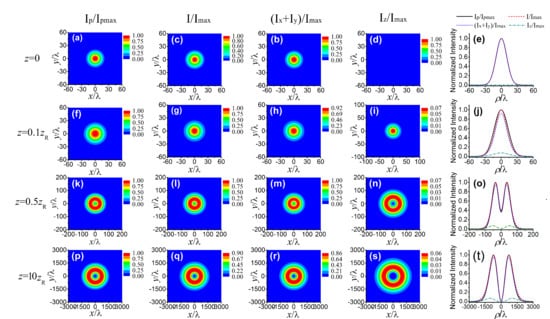
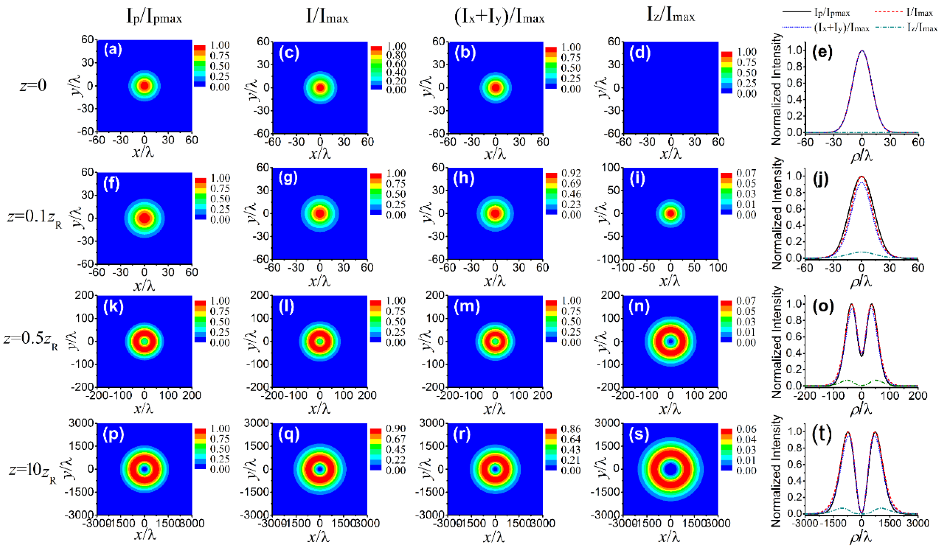
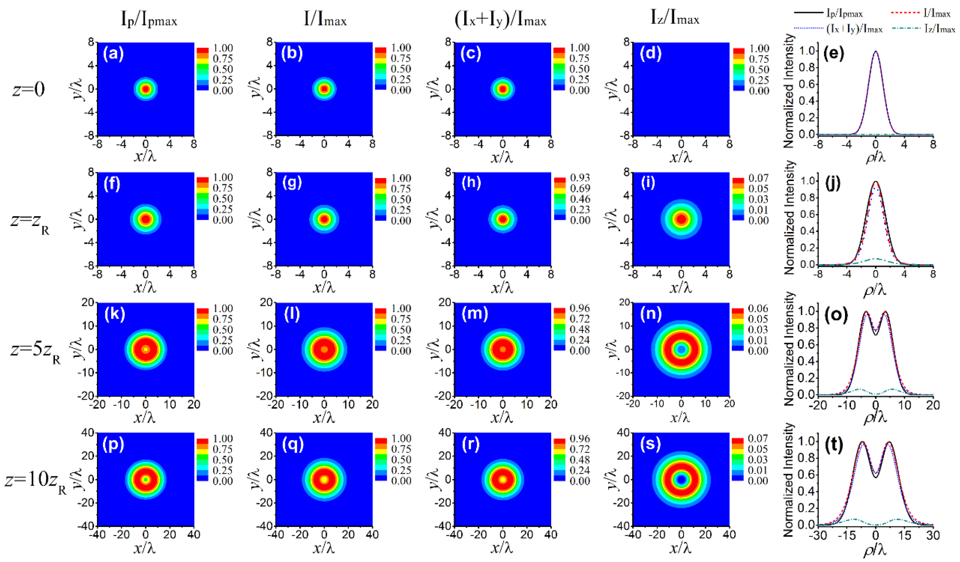
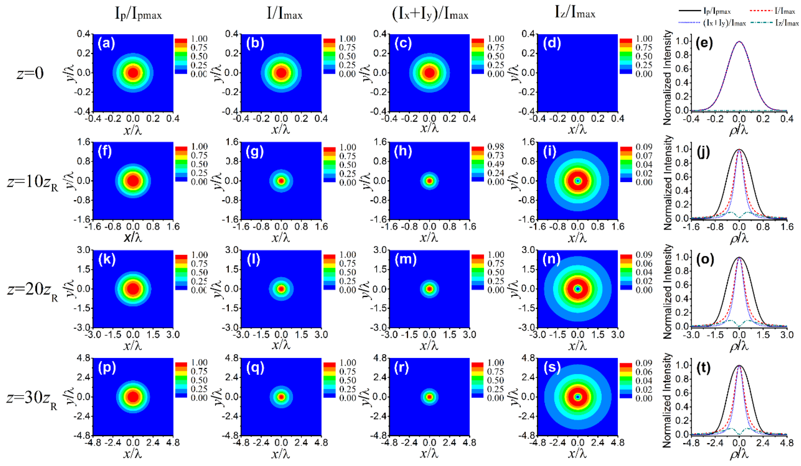
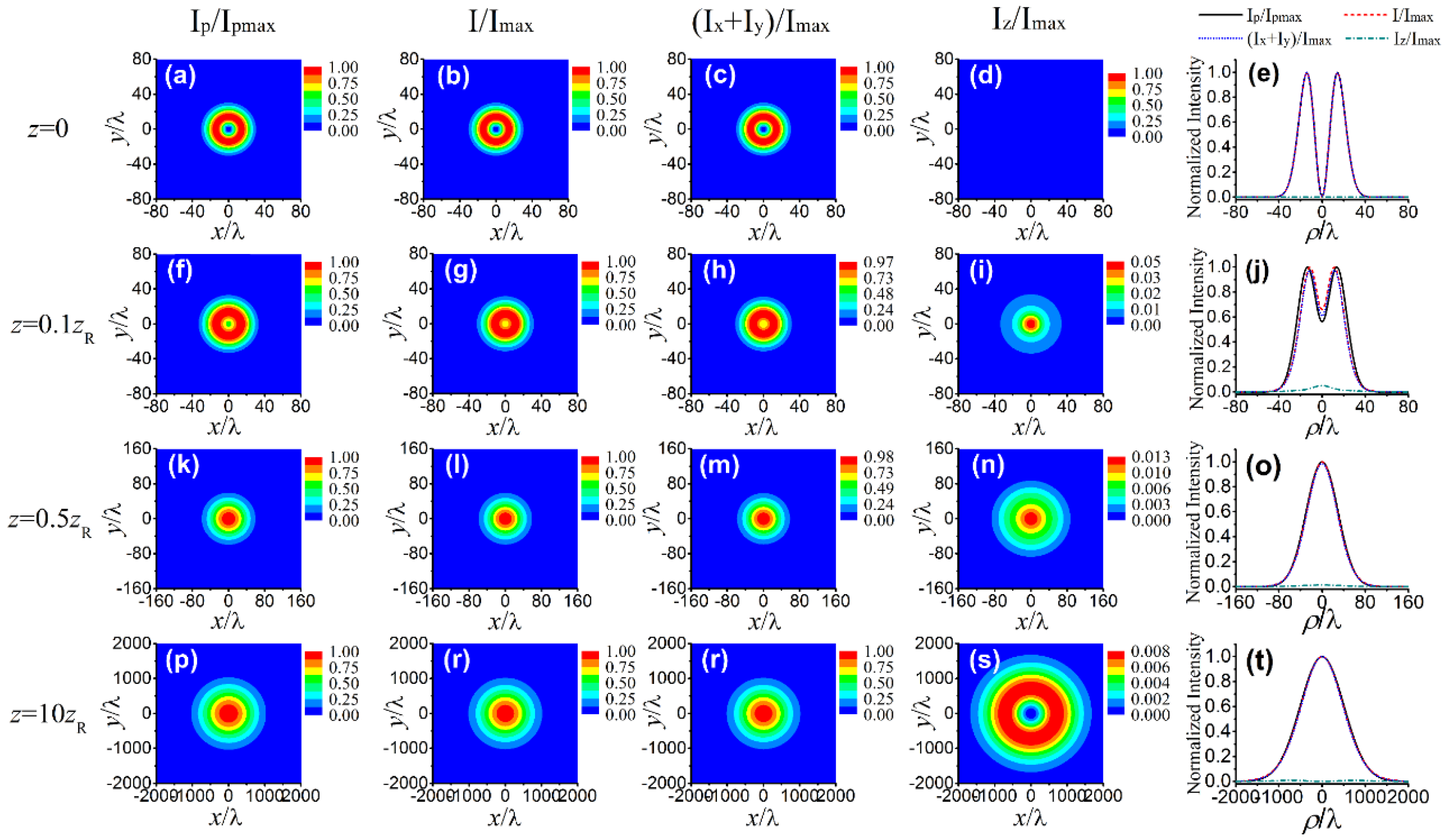
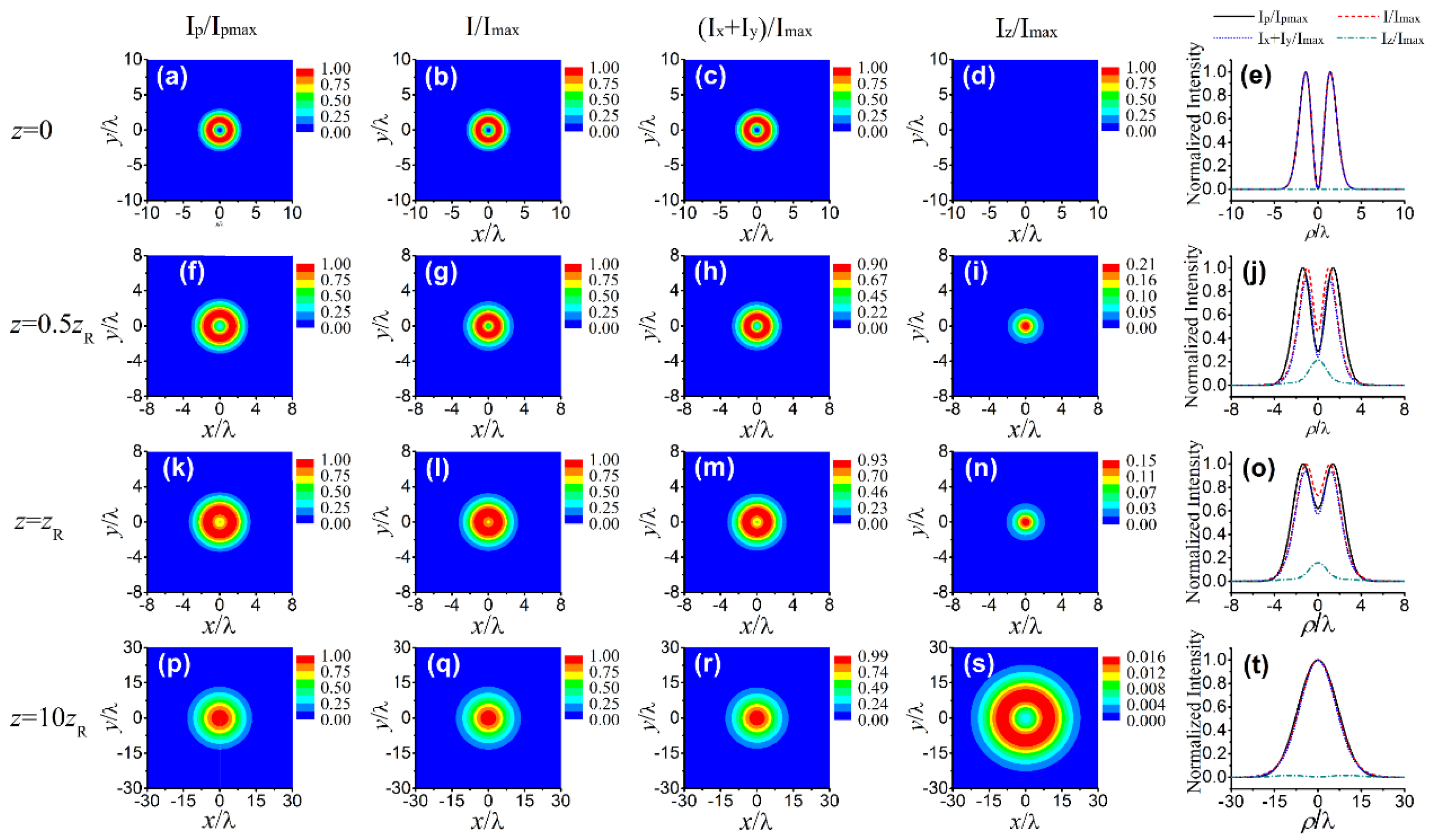
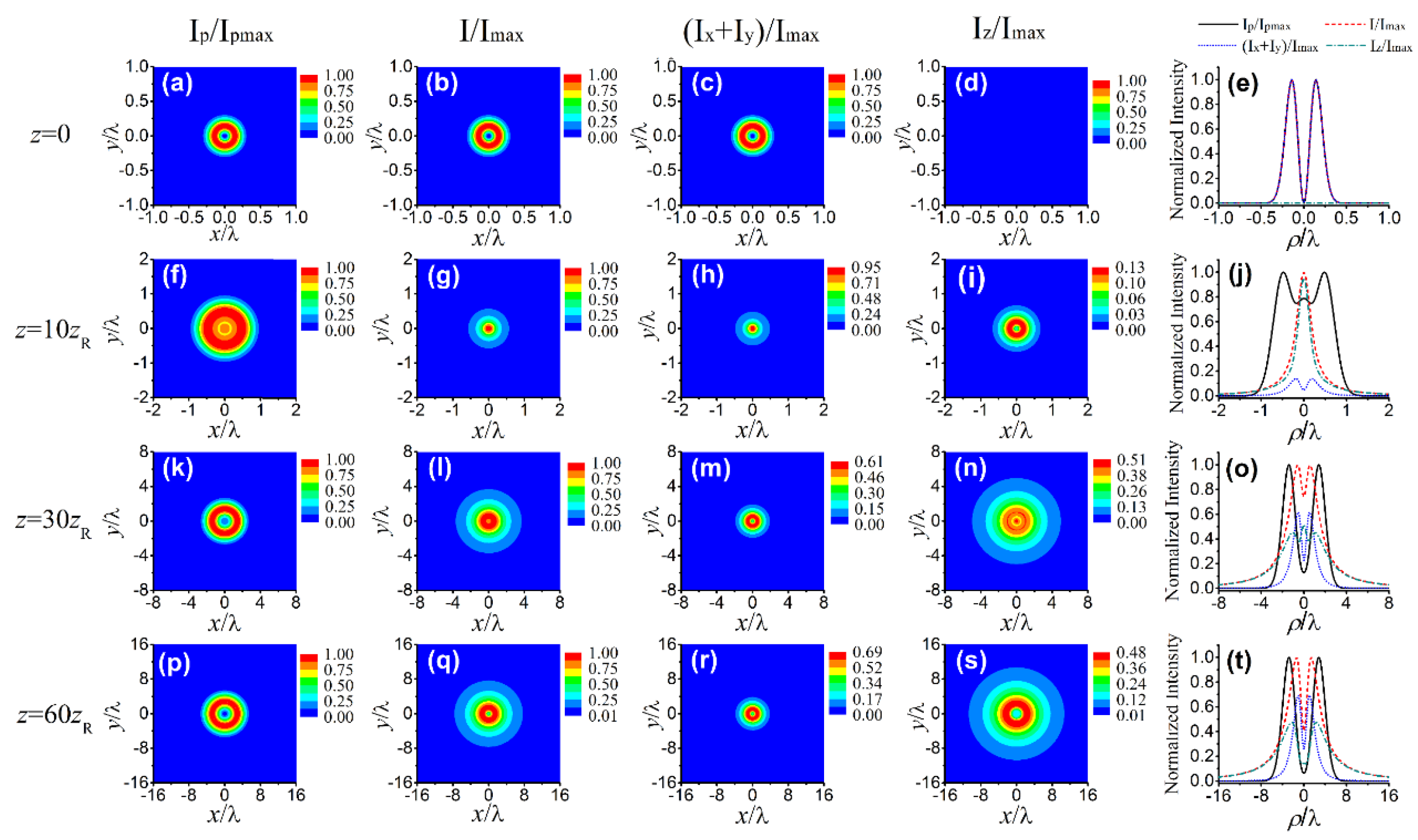
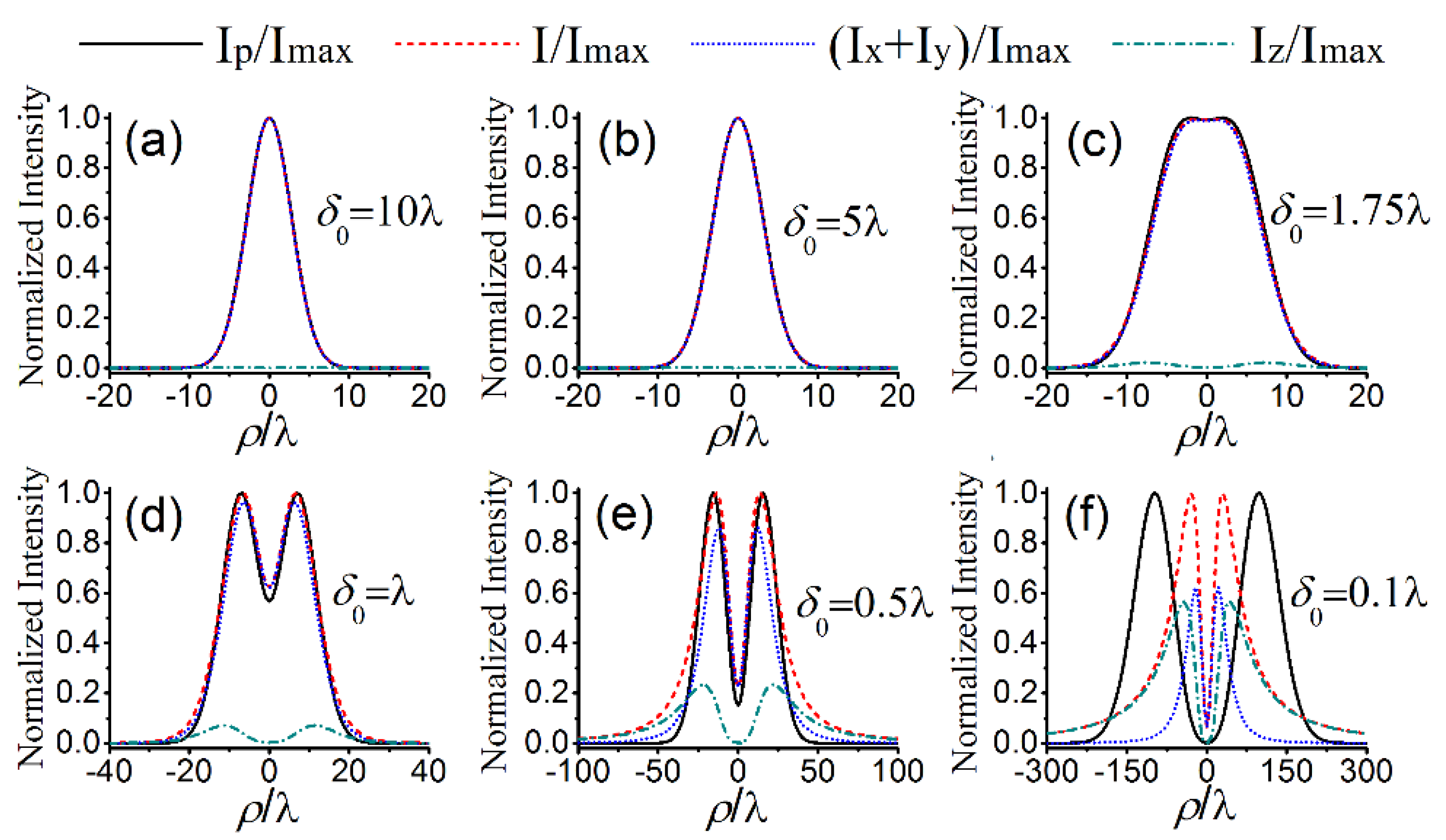
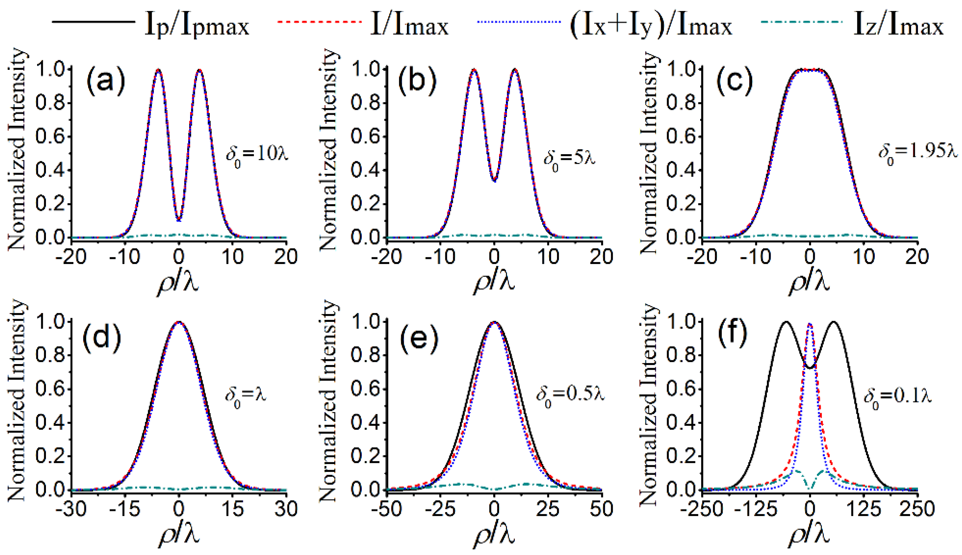
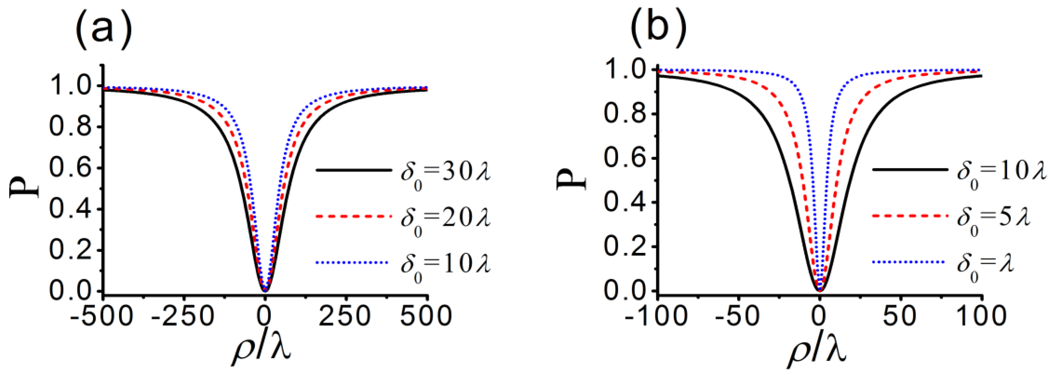
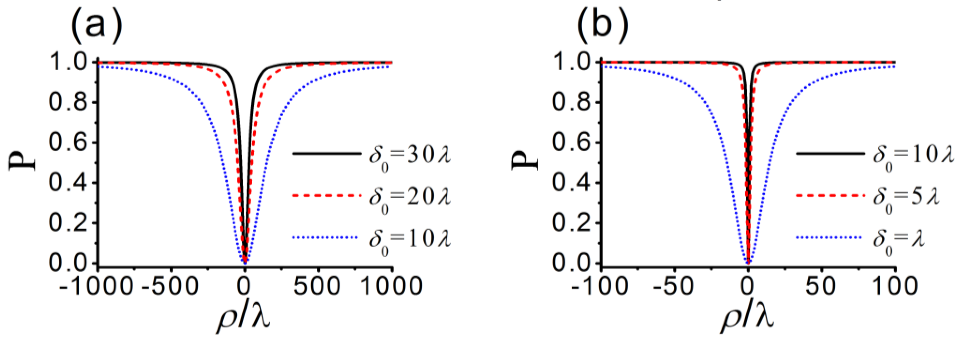
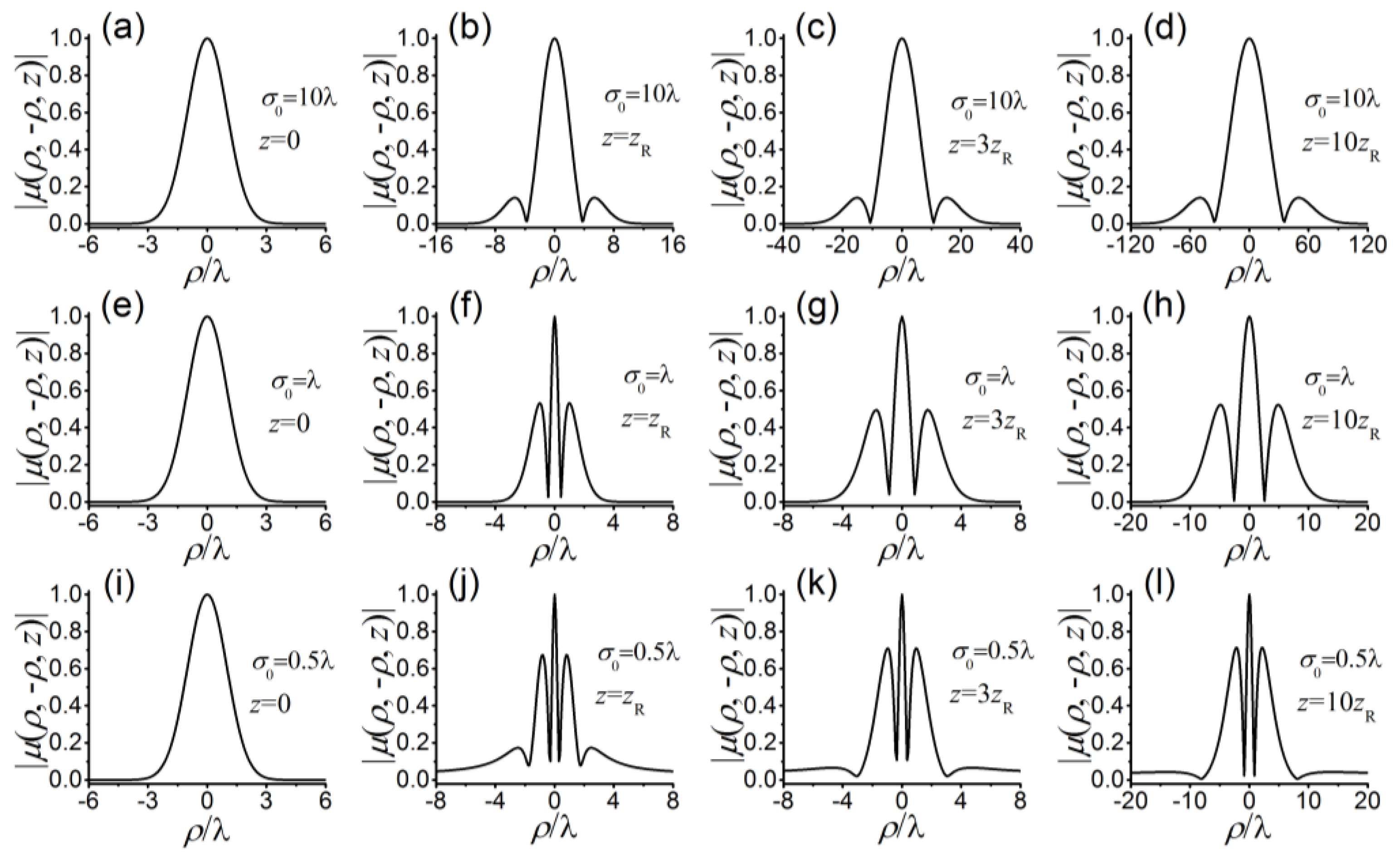
3. Statistical Properties of a Nonparaxial SCRP Beam

In this section, we will numerically study the statistical properties, such as the intensity, the degree of polarization, and the SDOC of a nonparaxial SCRP by applying the formulae derived in the above section. The statistical properties of a nonparaxial PCRP beam in free space are studied comparatively as well. In the following numerical examples, the propagation distances are normalized to z / z R , where z R = π σ 0 2 / λ is the Rayleigh distance.
Figure 1, Figure 2 and Figure 3 show the normalized intensity distributions I/Imax, (Ix + Iy)/Imax, and Iz/Imax and their corresponding cross lines ( y = x ) of a nonparaxial SCRP beam at different propagation distances for σ 0 = 10 λ , λ , and 0.1 λ , respectively. Figure 4, Figure 5 and Figure 6 show the contour graphs of Ip/Ipmax, I/Imax, (Ix + Iy)/Imax, and Iz/Imax and the corresponding cross lines ( y = x ) of a nonparaxial PCRP beam under the same parameter conditions as those in Figure 1, Figure 2 and Figure 3. The coherence widths of both SCRP and PCRP beams are set to δ 0 = λ . For the convenience of comparison, the normalized paraxial intensity distribution Ip/Ipmax of SCRP and PCRP beams and their corresponding cross lines ( y = x ) are also plotted in Figure 1, Figure 2 and Figure 3 and Figure 4, Figure 5 and Figure 6, respectively. Several interesting properties can be observed in these plots. First, from the comparison of Figure 1, Figure 2 and Figure 3, we find that the intensity in the far field (fourth row of each figure) of the nonparaxial SCPR beam is closely determined by the initial beam waist width σ 0 . When σ 0 is large, the far-field intensity is dark hollow (see Figure 1), while when σ 0 is small, the far-field intensity is a quasi-Gaussian distribution (see Figure 3). Very similar conclusions can be drawn for the nonparaxial PCRP beam (see Figure 4, Figure 5 and Figure 6). Second, the evolution properties of the intensity in the free space for the nonparaxial SCPR beam and the nonparaxial PCRP beam are totally different. From Figure 1, we find that for a nonparaxial SCPR beam, the total intensity changes gradually from a Gaussian shape to a dark hollow profile with the increase of the propagation distance. By contrast, from Figure 4, we find that for a nonparaxial PCRP beam, the total intensity changes gradually from a dark hollow shape to a Gaussian profile with the increase of the propagation distance. Furthermore, we find from Figure 1; Figure 4 that, in the case of σ 0 = 10 λ , there is a tiny discrepancy between nonparaxial and paraxial intensity distributions in the near and far fields due to the fact that Iz/Imax is extremely small compared to I/Imax, or (Ix + Iy)/Imax and can be negligible. In this case, the paraxial approximation is valid. However, for a very small value of σ 0 = 0.1 λ , as displayed in Figure 3 and Figure 6, the ratio of Iz/Imax becomes extremely noticeable and results in an appreciable discrepancy between nonparaxial and paraxial results in both near and far fields. Therefore, nonparaxial propagation formulae should be adopted to describe the propagation of SCRP and PCRP beams with a beam waist width that is much smaller than λ.
Next, we will investigate the effect of the spatial coherence on the propagation properties of both SCRP and PCRP beams. We plot in Figure 7 and Figure 8 the normalized intensity distribution of SCRP and PCRP beams at z = 10 z R , with σ 0 = λ for different values of spatial coherence width δ0. The corresponding paraxial results are also plotted together for comparison. One finds that the nonparaxiality of the SCRP and PCRP beams is also closely determined by their spatial coherence widths δ0. When δ0λ, the longitudinal component intensity Iz/Imax is negligible compared with I/Imax, or (Ix + Iy)/Imax, thus the paraxial approximation is allowable. However, with a decrease of δ0, the ratio of Iz/Imax increases quickly, for a very small value of σ 0 = 0.1 λ or 0.5 λ , the longitudinal component intensity Iz/Imax becomes extremely noticeable, and a notable discrepancy between the nonparaxial and paraxial results appears. A possible explanation is that a very small coherence width leads to a larger divergence angle, thus the beam becomes nonparaxial. In this case, the vectorial nonparaxiality of the SCRP and PCRP beams has to be taken into consideration. One can also find from Figure 7 and Figure 8 that the far-field intensity profiles of the SCRP and PCRP beams are also closely determined by their coherence length δ0. With the decrease of δ0, the beam profile of the SCRP field changes from Gaussian shape, to central-dark, flat-topped, and finally hollow beam spot, while the beam profile of the PCRP beam changes from hollow beam spot, to half-dark hollow beam spot, flat-topped, and finally Gaussian beam spot in the far field. Thus, one can shape the intensity distribution of nonparaxial SCRP and PCRP fields by modulating their initial spatial coherence, which is useful in material thermal processing and particle trapping.
Now, we can make some conclusions for the evolution of the intensity from Figure 1, Figure 2, Figure 3, Figure 4, Figure 5, Figure 6, Figure 7 and Figure 8. The nonparaxiality of the SCRP and PCRP beams is closely determined by both their initial beam waist sizes and their coherence widths. When both the beam waist sizes and the coherence widths are larger than the wavelength, the difference between the results calculated by the nonparaxial propagation formulas and those calculated by the paraxial propagation formulas can be negligible. If either the beam waist size or the coherence width is smaller than the wavelength, a significant difference appears, and nonparaxial propagation formulas are necessary for treating the propagation of SCRP and PCRP beams. Moreover, the modulation of the beam waist widths and the coherence widths on the profiles of the SCRP and PCPR beams in the far field is different.
Next, we turn to study the polarization properties of the nonparaxial SCRP beam in free space. We calculate in Figure 9 and Figure 10 the degrees of polarization of nonparaxial SCRP and PCRP beams at z = 10 z R for different δ 0 , respectively. The beam waist width in Figure 9a and Figure 10a is set to be σ 0 = 10 λ , which indicates the paraxial propagation, while, in Figure 9b and Figure 10b is selected as σ 0 = λ , which indicates the nonparaxial propagation. One finds that the degree polarization of both SCRP and PCRP beams, whether for paraxial or nonparaxial propagation, form an “Inverse Gaussian” shape during propagation, i.e., the SCRP and PCRP beams were depolarized, and the degree of polarization of increased as the transverse coordinate increased. The depolarization was attributed to the unneglectable z component and its limited spatial coherence length. What is interesting is that the evolution properties of the degree of polarization of the SCRP and PCRP beams are strikingly different, i.e., the degree of polarization of an SCPR beam increases as the initial coherence width decreases, while that of the PCRP beam decreases as the initial coherence width decreases. The difference arises from the different correlation structures (correlation matrix) of the SCRP and PCRP beams. A PCRP beam with a conventional Gaussian correlation structure will become less and less polarized with the increase of the propagation distance or the decrease of the initial coherence [74]. By contrast, a SCRP beam will become more and more polarized with the increase of the propagation distance or the decrease of the initial coherence. The physics behind this phenomenon has been discussed in detail in reference [21].
To learn about the SDOC of nonparaxial SCRP and PCRP beams on propagation, we comparatively calculate the modulus of the SDOC of nonparaxial SCRP and PCRP beams between two transverse points ( x , y ) and ( x , y ) at several propagation distances z with δ 0 = 2 λ for different values of σ 0 in Figure 11 and Figure 12, respectively. The beam waist widths in Figure 11a and Figure 12a are both chosen as σ 0 = 10 λ and indicate the paraxial propagation of the SCRP and PCRP beams, respectively. One sees clearly in Figure 11 that the evolution properties of SDOC of nonparaxial and paraxial SCRP beams are substantially different, i.e., with the increase of z, the distribution of the SDOC gradually degenerates from the initial non-Gaussian distribution with two sidelobes around the central bright spot into Gaussian distribution in the far field. However, the degeneration speed is higher with the decrease of σ0. On the other hand, we see clearly in Figure 12 that the evolution propagation of the SDOC for a PCRP beam is in contrast with that of an SCRP beam, i.e., the SDOC evolves from the initial Gaussian distribution into non-Gaussian distribution with two or four sidelobes around the central bright spot, and the evolution behaviors of the SDOC of nonparaxial and paraxial SCRP beams are different and related to σ0. The comparison shows that both the initial beam waist width and the coherence function play an important role in the evolution properties of the SDOC.

4. Conclusions

On the basis of the generalized vectorial Rayleigh–Sommerfeld diffraction integral formulas, analytical expressions for the 3 × 3 cross-spectral density matrix of an SCRP beam that propagates nonparaxially in free space has been derived. Furthermore, with the help of numerical calculations, the intensity, polarization, and SDOC of an SCRP beam have been illustrated and compared with those of a PCRP beam. It was found that the intensity distribution, degree of polarization, and SDOC of nonparaxial SCPR and PCRP beams determined by their beam waist width and spatial correlation function are substantially different. Therefore, by modulating the initial beam waist width and spatial correlation function, one can modulate the statistical properties of a nonparaxial partially coherent vector field. When we go a step further, the nonparaxial statistical properties can be used to manipulate the optical forces induced by the interaction of the optical fields and the nanoparticles [30,31,45]. Therefore, our findings can have potential use in nanoparticle trapping in nonparaxial systems.

Author Contributions

L.G. (Data curation, Writing—original draft); L.C. (Formal analysis, writing—original draft preparation); R.L. (Supervision, Writing-review and editing); M.Z. (Validation, Writing—review and editing); Y.D. (software, Validation); Y.Chen (Formal analysis, Writing—review and editing); Y.Cai (Supervision, Project administration, Writing—review and editing).

Funding

This research was funded by the National Natural Science Fund for Distinguished Young Scholar [11525418], the National Natural Science Foundation of China [91750201], Characteristic Innovation Project (Natural Science) of the Education Department of Guangdong Province [2017KTSCX114].

Conflicts of Interest

The authors declare no conflict of interest.

Appendix A

The elements of the CSD matrix of a PCRP beam in source plane z = 0 reads as [8,38,75]:
W α α ( x 10 , y 10 , x 20 , y 20 , 0 ) = α 10 α 20 4 σ 0 2 exp ( r 10 2 + r 20 2 4 σ 0 2 ) exp [ ( r 10 r 20 ) 2 2 δ 0 2 ] , ( α = x , y )
W x y ( x 10 , y 10 , x 20 , y 20 , 0 ) = x 10 y 20 4 σ 0 2 exp ( r 10 2 + r 20 2 4 σ 0 2 ) exp [ ( r 10 r 20 ) 2 2 δ 0 2 ] ,
W y x ( x 10 , y 10 , x 20 , y 20 , 0 ) = W x y * ( x 20 , y 20 , x 10 , y 10 , 0 ) ,
Substituting Equations (A1)–(A3) and (14) into Equations (11)–(13), following a similar procedure of the derivation of the beam coherence polarization (BCP) matrix of the SCRP beam, the elements of the CSD matrix of the PCRP beam in free space can be derived as:
W α α ( x 1 , y 1 , x 2 , y 2 , z ) = z 2 Δ 4 M N δ 0 2 ( 1 + b α 2 2 M i k δ 0 2 α 2 b α r 2 ) , ( α = x , y )
W x y ( x 1 , y 1 , x 2 , y 2 , z ) = z 2 Δ 4 M N δ 0 2 ( b x b y 2 M i k δ 0 2 y 2 b x r 2 ) ,
W y x ( x 1 , y 1 , x 2 , y 2 , z ) = W x y ( x 2 , y 2 , x 1 , y 1 , z ) ,
W α z ( x 1 , y 1 , x 2 , y 2 , z ) = z Δ [ A α 0 Q α 1 + A α 1 Q α 2 + A α 2 Q α 3 + k b α 2 M ( A β 0 + A β 1 Q β 1 + A β 2 Q β 2 ) ] , ( α , β = x , y )
W z α ( x 1 , y 1 , x 2 , y 2 , z ) = W α z ( x 2 , y 2 , x 1 , y 1 , z ) ,
W z z ( x 1 , y 1 , x 2 , y 2 , z ) = Δ [ W z x x ( x 1 , y 1 , x 2 , y 2 , z ) + W z x y ( x 1 , y 1 , x 2 , y 2 , z ) + W z y x ( x 1 , y 1 , x 2 , y 2 , z ) + W z y y ( x 1 , y 1 , x 2 , y 2 , z ) ]
with
W z α α ( x 1 , y 1 , x 2 , y 2 , z ) = A α 0 α 1 Q α 1 + ( A α 1 α 1 A α 0 ) Q α 2 + ( A α 2 α 1 A α 1 ) Q α 3 A α 2 Q α 4 W z α β ( x 1 , y 1 , x 2 , y 2 , z ) = ( α 1 Q α 1 Q α 2 ) ( A β 0 + A β 1 Q β 1 + A β 2 Q β 2 ) Δ = 1 4 σ 0 2 Δ , A α 0 = k 2 α 2 2 4 N 2 r 2 2 i k α 2 2 2 N r 2 1 2 N A α 1 = α 2 2 N δ 0 2 + i k α 2 2 N 2 r 2 δ 0 2 , A α 2 = 1 4 N 2 δ 0 4 ,
Under the paraxial condition r j z + ( x j 2 + y j 2 ) / 2 z , (j = 1, 2), Equations (A4)—(A6) can reduce to the propagation formulas for the elements of the 2 × 2 CSD matrix of a paraxial PCRP beam in free space, which are consistent with the result in the Equation (6) in reference [75]. On the basis of the derived formula shown in Equations (A4)–(A9), the statistical properties such as intensity, degree of polarization, and SDOC of the nonparaxial PCRP beam in free space can be determined.

References

  1. Zhan, Q. Cylindrical vector beams: From mathematical concepts to applications. Adv. Opt. Photonics 2009, 1, 1–57. [Google Scholar] [CrossRef]
  2. Ehmke, T.; Nitzsche, T.H.; Knebl, A.; Heisterkamp, A. Molecular orientation sensitive second harmonic microscopy by radially and azimuthally polarized light. Biomed. Opt. Express 2014, 5, 2231–2246. [Google Scholar] [CrossRef] [PubMed]
  3. Dorn, R.; Quabis, S.; Leuchs, G. Sharper focus for a radially polarized light beam. Phys. Rev. Lett. 2003, 91, 233901. [Google Scholar] [CrossRef] [PubMed]
  4. Zhan, Q. Radiation forces on a dielectric sphere produced by highly focused cylindrical vector beams. J. Opt. A 2003, 5, 229–232. [Google Scholar] [CrossRef]
  5. Jia, B.; Kang, H.; Li, J.; Gu, M. Use of radially polarized beams in three-dimensional photonic crystal fabrication with the two-photon polymerization method. Opt. Lett. 2009, 34, 1918–1920. [Google Scholar] [CrossRef] [PubMed]
  6. Ahmadivand, A.; Gerislioglu, B.; Pala, N. Azimuthally and radially excited charge transfer plasmon and Fano lineshapes in conductive sublayer-mediated nanoassemblies. J. Opt. Soc. Am. A 2017, 34, 2052–2056. [Google Scholar] [CrossRef] [PubMed]
  7. Xu, J.; Li, K.; Zhang, S.; Lu, X.; Shi, N.; Tan, Z.; Lu, Y.; Liu, N.; Zhang, B.; Liang, Z. Field-enhanced nanofocusing of radially polarized light by a tapered hybrid plasmonic waveguide with periodic grooves. Appl. Opt. 2019, 58, 588–592. [Google Scholar] [CrossRef] [PubMed]
  8. Dong, Y.; Cai, Y.; Zhao, C.; Yao, M. Statistics properties of a cylindrical vector partially coherent beam. Opt. Express 2011, 19, 5979–5992. [Google Scholar] [CrossRef] [PubMed]
  9. Wang, F.; Cai, Y.; Dong, Y.; Korotkova, O. Experimental generation of a radially polarized beam with controllable spatial coherence. Appl. Phys. Lett. 2012, 100, 051108. [Google Scholar] [CrossRef]
  10. Wang, F.; Liu, X.; Liu, L.; Yuan, Y.; Cai, Y. Experimental study of the scintillation index of a radially polarized beam with controllable spatial coherence. Appl. Phys. Lett. 2013, 103, 091102. [Google Scholar] [CrossRef]
  11. Guo, L.; Chen, Y.; Liu, X.; Liu, L.; Cai, Y. Vortex phase-induced changes of the statistical properties of a partially coherent radially polarized beam. Opt. Express 2016, 24, 13714–13728. [Google Scholar] [CrossRef] [PubMed]
  12. Liu, L.; Peng, X.; Chen, Y.; Guo, L.; Cai, Y. Statistical properties of a radially polarized twisted Gaussian Schell-model beam in a uniaxial crystal. J. Mod. Opt. 2017, 64, 698–708. [Google Scholar] [CrossRef]
  13. Zhang, Y.; Cui, Y.; Wang, F.; Cai, Y. Correlation singularities in a partially coherent electromagnetic beam with initially radial polarization. Opt. Express 2015, 23, 11483–11492. [Google Scholar] [CrossRef] [PubMed]
  14. Zhu, S.; Wang, F.; Chen, Y.; Li, Z.; Cai, Y. Statistical properties in Young’s interference pattern formed with a radially polarized beam with controllable spatial coherence. Opt. Express 2014, 22, 28697–28710. [Google Scholar] [CrossRef] [PubMed]
  15. Cai, Y.; Chen, Y.; Wang, F. Generation and propagation of partially coherent beams with nonconventional correlation functions: A review [invited]. J. Opt. Soc. Am. A 2014, 31, 2083–2096. [Google Scholar] [CrossRef] [PubMed]
  16. Mei, Z.; Korotkova, O. Random sources generating ring-shaped beams. Opt. Lett. 2013, 38, 91–93. [Google Scholar] [CrossRef] [PubMed]
  17. Yu, J.; Cai, Y.; Gbur, G. Rectangular Hermite non-uniformly correlated beams and its propagation properties. Opt. Express 2018, 26, 27894–27906. [Google Scholar] [CrossRef] [PubMed]
  18. Wang, F.; Liang, C.; Cai, Y.; Yuan, Y. Generalized multi-Gaussian correlated Schell-model beam: From theory to experiment. Opt. Express 2014, 22, 23456–23464. [Google Scholar] [CrossRef] [PubMed]
  19. Chen, Y.; Wang, F.; Yu, J.; Liu, L.; Cai, Y. Vector Hermite-Gaussian correlated Schell-model beam. Opt. Express 2016, 24, 15232–15250. [Google Scholar] [CrossRef] [PubMed]
  20. Zhao, D.; Wan, L. Optical coherence grids and their propagation characteristics. Opt. Express 2018, 26, 2168–2180. [Google Scholar] [CrossRef]
  21. Chen, Y.; Wang, F.; Liu, L.; Zhao, C.; Cai, Y.; Korotkova, O. Generation and propagation of a partially coherent vector beam with special correlation functions. Phys. Rev. A 2014, 89, 013801. [Google Scholar] [CrossRef]
  22. Zhang, J.; Wang, J.; Huang, H.; Wang, H.; Zhu, S.; Li, Z.; Lu, J. Propagation Characteristics of a Twisted Cosine-Gaussian Correlated Radially Polarized Beam. Appl. Sci. 2018, 8, 1485. [Google Scholar] [CrossRef]
  23. Santarsiero, F.; Gori, M. Devising genuine spatial correlation functions. Opt. Lett. 2007, 32, 3531–3533. [Google Scholar] [CrossRef]
  24. Gori, F.; Ramírezsánchez, V.; Santarsiero, M.; Shirai, T. On genuine cross-spectral density matrices. J. Opt. A 2009, 11, 85706–85707. [Google Scholar] [CrossRef]
  25. Martínez-Herrero, R.; Mejías, P.; Gori, F. Genuine cross-spectral densities and pseudo-modal expansions. Opt. Lett. 2009, 34, 1399–1401. [Google Scholar] [CrossRef] [PubMed]
  26. Martínez-Herrero, R.; Mejías, P.M. Elementary-field expansions of genuine cross-spectral density matrices. Opt. Lett. 2009, 34, 2303–2305. [Google Scholar] [CrossRef] [PubMed]
  27. Wang, F.; Yu, J.; Liu, X.; Cai, Y. Research progress of partially coherent beams propagation in turbulent atmosphere. Acta Phys. Sin. 2018, 67, 184203. [Google Scholar] [CrossRef]
  28. Liang, C.; Wu, G.; Wang, F.; Li, W.; Cai, Y.; Ponomarenko, S.A. Overcoming the classical Rayleigh diffraction limit by controlling two-point correlations of partially coherent light sources. Opt. Express 2017, 25, 28352–28362. [Google Scholar] [CrossRef]
  29. Yu, J.; Wang, F.; Liu, L.; Cai, Y.; Gbur, G. Propagation properties of Hermite non-uniformly correlated beams in turbulence. Opt. Express 2018, 26, 27894–27906. [Google Scholar] [CrossRef] [PubMed]
  30. Zhou, Y.; Xu, H.F.; Yuan, Y.; Peng, J.; Qu, J.; Huang, W. Trapping two types of particles using a Laguerre-Gaussian correlated Schell-model beam. IEEE Photon. J. 2016, 8, 1–10. [Google Scholar] [CrossRef]
  31. Liu, X.; Zhao, D. Trapping two types of particles with a focused generalized Multi-Gaussian Schell model beam. Opt. Commun. 2015, 354, 250–255. [Google Scholar] [CrossRef]
  32. Dao, W.; Liang, C.; Wang, F.; Cai, Y.; Hoenders, B. Effects of Anisotropic Turbulence on Propagation Characteristics of Partially Coherent Beams with Spatially Varying Coherence. Appl. Sci. 2018, 8, 2025. [Google Scholar] [CrossRef]
  33. Rubinsztein-Dunlop, H.; Forbes, A.; Berry, M.V.; Dennis, M.R.; Andrews, D.L.; Mansuripur, M.; Denz, C.; Alpmann, C.; Banzer, P.; Bauer, T. Roadmap on structured light. J. Opt. 2016, 19, 013001. [Google Scholar] [CrossRef] [Green Version]
  34. Dholakia, K.; Čižmár, T. Shaping the future of manipulation. Nat. Photon. 2011, 5, 335. [Google Scholar] [CrossRef]
  35. Leach, J.; Jack, B.; Romero, J.; Jha, A.K.; Yao, A.M.; Franke-Arnold, S.; Ireland, D.G.; Boyd, R.W.; Barnett, S.M.; Padgett, M. Quantum correlations in optical angle–orbital angular momentum variables. Science 2010, 329, 662–665. [Google Scholar] [CrossRef] [PubMed]
  36. Sarenac, D.; Cory, D.G.; Nsofini, J.; Hincks, I.; Miguel, P.; Arif, M.; Clark, C.W.; Huber, M.G.; Pushin, D.A. Generation of a lattice of spin-orbit beams via coherent averaging. Phys. Rev. Lett. 2018, 121, 183602. [Google Scholar] [CrossRef] [PubMed]
  37. Cui, Y.; Wei, C.; Zhang, Y.; Wang, F.; Cai, Y. Effect of the atmospheric turbulence on a special correlated radially polarized beam on propagation. Opt. Commun. 2015, 354, 353–361. [Google Scholar] [CrossRef]
  38. Wang, F.; Chen, Y.; Liu, X.; Cai, Y.; Ponomarenko, S.A. Self-reconstruction of partially coherent light beams scattered by opaque obstacles. Opt. Express 2016, 24, 23735–23746. [Google Scholar] [CrossRef] [PubMed]
  39. Naqwi, A.; Durst, F. Focusing of diode laser beams: A simple mathematical model. Appl. Opt. 1990, 29, 1780–1785. [Google Scholar] [CrossRef] [PubMed]
  40. Borghi, R.; Santarsiero, M.; Alonso, M.A. Highly focused spirally polarized beams. J. Opt. Soc. Am. A 2005, 22, 1420–1431. [Google Scholar] [CrossRef]
  41. Chaumet, P.C. Vision. Fully vectorial highly nonparaxial beam close to the waist. J. Opt. Soc. Am. A 2006, 23, 3197–3202. [Google Scholar] [CrossRef]
  42. Zhang, P.; Hu, Y.; Cannan, D.; Salandrino, A.; Li, T.; Morandotti, R.; Zhang, X.; Chen, Z. Generation of linear and nonlinear nonparaxial accelerating beams. Opt. Lett. 2012, 37, 2820–2822. [Google Scholar] [CrossRef] [PubMed]
  43. Alexandre, A.; Michel, P. 4π Focusing of TM(01) beams under nonparaxial conditions. Opt. Express 2010, 18, 22128–22140. [Google Scholar] [CrossRef]
  44. Moon, H.J.; Chough, Y.T.; An, K. Cylindrical microcavity laser based on the evanescent-wave-coupled gain. Phys. Rev. Lett. 2000, 85, 3161–3164. [Google Scholar] [CrossRef] [PubMed]
  45. Sung, S.-Y.; Lee, Y.-G. Trapping of a micro-bubble by non-paraxial Gaussian beam: Computation using the FDTD method. Opt. Express 2008, 16, 3463–3473. [Google Scholar] [CrossRef] [PubMed]
  46. Balázs, G.; Pál, K.; Attila, B.G.; Emőke, L. Computer simulation of reflective volume grating holographic data storage. J. Opt. Soc. Am. A 2007, 24, 2075–2081. [Google Scholar] [CrossRef]
  47. Kuittinen, M.; Vahimaa, P.; Honkanen, M.; Turunen, J. Beam shaping in the nonparaxial domain of diffractive optics. Appl. Opt. 1997, 36, 2034–2041. [Google Scholar] [CrossRef] [PubMed]
  48. Sung, Y.; Sheppard, C.J.R. Three-dimensional imaging by partially coherent light under nonparaxial condition. J. Opt. Soc. Am. A 2011, 28, 554–559. [Google Scholar] [CrossRef] [PubMed]
  49. Duan, K.; Lü, B. Wigner-distribution-function matrix and its application to partially coherent vectorial nonparaxial beams. J. Opt. Soc. Am. B 2005, 22, 1585–1593. [Google Scholar] [CrossRef]
  50. Porras, M.A. Non-paraxial vectorial moment theory of light beam propagation. Opt. Commun. 1996, 127, 79–95. [Google Scholar] [CrossRef]
  51. Duan, K.; Lü, B. Partially coherent vectorial nonparaxial beams. J. Opt. Soc. Am. A 2004, 21, 1924–1932. [Google Scholar] [CrossRef]
  52. Ciattoni, A.; Porto, P.D.; Crosignani, B.; Yariv, A. Vectorial nonparaxial propagation equation in the presence of a tensorial refractive-index perturbation. J. Opt. Soc. Am. B 2000, 17, 809–819. [Google Scholar] [CrossRef]
  53. Luneburg, R.K. Mathematical Theory of Optics; University of California Press: Berkeley, CA, USA, 1966. [Google Scholar]
  54. Wang, X.; Liu, Z.; Zhao, D. Nonparaxial propagation of Lorentz-Gauss beams in uniaxial crystal orthogonal to the optical axis. J. Opt. Soc. Am. A 2014, 31, 872–878. [Google Scholar] [CrossRef] [PubMed]
  55. Zhang, P.; Hu, Y.; Li, T.; Cannan, D.; Yin, X.; Morandotti, R.; Chen, Z.; Zhang, X. Nonparaxial Mathieu and Weber Accelerating Beams. Phys. Rev. Lett. 2012, 109, 193901. [Google Scholar] [CrossRef] [PubMed] [Green Version]
  56. Deng, D.; Gao, Y.; Zhao, J.; Zhang, P.; Chen, Z. Three-dimensional nonparaxial beams in parabolic rotational coordinates. Opt. Lett. 2013, 38, 3934–3936. [Google Scholar] [CrossRef] [PubMed]
  57. Volyar, A.V.; Fadeeva, T.A.; Shvedov, V.G. Topological phase in a nonparaxial Gaussian beam. Tech. Phys. Lett. 1999, 25, 891–893. [Google Scholar] [CrossRef]
  58. Klaassen, T.; Hoogeboom, A.; van Exter, M.P.; Woerdman, J.P. Gouy phase of nonparaxial eigenmodes in a folded resonator. J. Opt. Soc. Am. A 2004, 21, 1689–1693. [Google Scholar] [CrossRef]
  59. Kotlyar, V.V.; Kovalev, A.A.; Soifer, V.A. Nonparaxial Hankel vortex beams of the first and second types. Comp. Opt. 2015, 39, 299–304. [Google Scholar] [CrossRef]
  60. Deng, D.; Guo, Q.; Wu, L.; Yang, X. Propagation of radially polarized elegant light beams. J. Opt. Soc. Am. B 2007, 24, 636–643. [Google Scholar] [CrossRef]
  61. Kovalev, A.A.; Kotlyar, V.V. Nonparaxial propagation of a Gaussian optical vortex with initial radial polarization. J. Opt. Soc. Am. A 2010, 27, 372–380. [Google Scholar] [CrossRef]
  62. Santarsiero, M.; Borghi, R. Nonparaxial propagation of spirally polarized optical beams. J. Opt. Soc. Am. A 2004, 21, 2029–2037. [Google Scholar] [CrossRef]
  63. Dong, Y.; Feng, F.; Chen, Y.; Zhao, C.; Cai, Y. Statistical properties of a nonparaxial cylindrical vector partially coherent field in free space. Opt. Express 2012, 20, 15908–15927. [Google Scholar] [CrossRef] [PubMed]
  64. Yuan, Y.; Du, S.; Dong, Y.; Wang, F.; Zhao, C.; Cai, Y. Nonparaxial propagation properties of a vector partially coherent dark hollow beam. J. Opt. Soc. Am. A 2013, 30, 1358–1372. [Google Scholar] [CrossRef] [PubMed]
  65. Zhang, L.; Cai, Y. Propagation of a twisted anisotropic Gaussian Schell-model beam beyond the paraxial approximation. Appl. Phys. B 2010, 103, 1001–1008. [Google Scholar] [CrossRef]
  66. Mandel, L.; Wolf, E. Optical Coherence and Quantum Optics; Cambridge university press: Cambridge, UK, 1995; ISBN 0521417112. [Google Scholar]
  67. Ciattoni, A.; Crosignani, B.; Porto, P.D. Vectorial analytical description of propagation of a highly nonparaxial beam. Opt. Commun. 2002, 202, 17–20. [Google Scholar] [CrossRef]
  68. Lü, B.; Duan, K. Nonparaxial propagation of vectorial Gaussian beams diffracted at a circular aperture. Opt. Lett. 2003, 28, 2440–2442. [Google Scholar] [CrossRef] [PubMed]
  69. Gradshteyn, I.S.; Ryzhik, I.M. Table of Integrals, Series, and Products, 7th ed.; Jeffrey, A., Zwillinger, D., Eds.; Academic press: London, UK, 2007; ISBN 9780123736376. [Google Scholar]
  70. Lindfors, K.; Setälä, T.; Kaivola, M.; Friberg, A.T. Degree of polarization in tightly focused optical fields. J. Opt. Soc. Am. A 2005, 22, 561–568. [Google Scholar] [CrossRef]
  71. Ellis, J.; Dogariu, A.; Ponomarenko, S.; Wolf, E. Degree of polarization of statistically stationary electromagnetic fields. Opt. Commun. 2005, 248, 333–337. [Google Scholar] [CrossRef]
  72. Setälä, T.; Shevchenko, A.; Kaivola, M.; Friberg, A.T. Degree of polarization for optical near fields. Phys. Rev. E 2002, 66, 016615. [Google Scholar] [CrossRef] [PubMed]
  73. Korotkova, O.; Wolf, E. Spectral degree of coherence of a random three-dimensional electromagnetic field. J. Opt. Soc. Am. A 2004, 21, 2382–2385. [Google Scholar] [CrossRef]
  74. Wu, G.; Wang, F.; Cai, Y. Coherence and polarization properties of a radially polarized beam with variable spatial coherence. Opt. Express 2012, 20, 28301–28318. [Google Scholar] [CrossRef] [PubMed]
  75. Qiu, Y.; Liu, J.; Chen, Z. Propagation properties of radially polarized partially coherent LG (0, 1) beams. Opt. Commun. 2009, 282, 69–73. [Google Scholar] [CrossRef]
Figure 1. Intensity distributions of the paraxial specially correlated radially polarized (SCRP) beam and the nonparaxial SCRP beam at the propagation distances z = 0 (first row), z = 0.1 z R (second row), z = 0.5 z R (third row), z = 10 z R (fourth row) in free space, where z R is the Rayleigh distance. First column: the total intensity Ip for the paraxial SCRP beam. Second column: the total intensity I for the nonparaxial SCRP beam. Third column: the transverse intensity Ix + Iy for the nonparaxial SCRP beam. Fourth column: the longitudinal intensity Iz for the nonparaxial SCRP beam. Fifth column: the corresponding cross lines ( y = x ) with ρ = x 2 + y 2 . Here, the beam width σ 0 = 10 λ , and the intensities are normalized with respect to their maxima.
Applsci 09 00997 g001
Figure 2. Intensity distributions of the SCRP beam and the nonparaxial SCRP beam at the propagation distances z = 0 (first row), z = 0.1 z R (second row), z = 0.5 z R (third row), z = 10 z R (fourth row) in free space, where z R is the Rayleigh distance. First column: the total intensity Ip for the paraxial SCRP beam. Second column: the total intensity I for the nonparaxial SCRP beam. Third column: the transverse intensity Ix + Iy for the nonparaxial SCRP beam. Fourth column: the longitudinal intensity Iz for the nonparaxial SCRP beam. Fifth column: the corresponding cross lines ( y = x ) with ρ = x 2 + y 2 . Here, the beam width σ 0 = λ , and the intensities are normalized with respect to their maxima.
Applsci 09 00997 g002
Figure 3. Intensity distributions of the SCRP beam and the nonparaxial SCRP beam at the propagation distances z = 0 (first row), z = 0.1 z R (second row), z = 0.5 z R (third row), z = 10 z R (fourth row) in free space, where z R is the Rayleigh distance. First column: the total intensity Ip for the paraxial SCRP beam. Second column: the total intensity I for the nonparaxial SCRP beam. Third column: the transverse intensity Ix + Iy for the nonparaxial SCRP beam. Fourth column: the longitudinal intensity Iz for the nonparaxial SCRP beam. Fifth column: the corresponding cross lines ( y = x ) with ρ = x 2 + y 2 . Here, the beam width σ 0 = 0.1 λ , and the intensities are normalized with respect to their maximums.
Applsci 09 00997 g003
Figure 4. Intensity distributions of the paraxial partially coherent radially polarized (PCRP) beam and the nonparaxial PCRP beam at the propagation distances z = 0 (first row), z = 0.1 z R (second row), z = 0.5 z R (third row), z = 10 z R (fourth row) in free space, where z R is the Rayleigh distance. First column: the total intensity Ip for the paraxial SCRP beam. Second column: the total intensity I for the nonparaxial SCRP beam. Third column: the transverse intensity Ix + Iy for the nonparaxial SCRP beam. Fourth column: the longitudinal intensity Iz for the nonparaxial SCRP beam. Fifth column: the corresponding cross lines ( y = x ) with ρ = x 2 + y 2 . Here, the beam width σ 0 = 10 λ , and the intensities are normalized with respect to their maximums.
Applsci 09 00997 g004
Figure 5. Intensity distributions of the PCRP beam and the nonparaxial PCRP beam at the propagation distances z = 0 (first row), z = 0.1 z R (second row), z = 0.5 z R (third row), z = 10 z R (fourth row) in free space, where z R is the Rayleigh distance. First column: the total intensity Ip for the paraxial SCRP beam. Second column: the total intensity I for the nonparaxial SCRP beam. Third column: the transverse intensity Ix + Iy for the nonparaxial SCRP beam. Fourth column: the longitudinal intensity Iz for the nonparaxial SCRP beam. Fifth column: the corresponding cross lines ( y = x ) with ρ = x 2 + y 2 . Here, the beam width σ 0 = λ , and the intensities are normalized with respect to their maximums.
Applsci 09 00997 g005
Figure 6. Intensity distributions of the PCRP beam and the nonparaxial PCRP beam at the propagation distances z = 0 (first row), z = 0.1 z R (second row), z = 0.5 z R (third row), z = 10 z R (fourth row) in free space, where z R is the Rayleigh distance. First column: the total intensity Ip for the paraxial SCRP beam. Second column: the total intensity I for the nonparaxial SCRP beam. Third column: the transverse intensity Ix + Iy for the nonparaxial SCRP beam. Fourth column: the longitudinal intensity Iz for the nonparaxial SCRP beam. Fifth column: the corresponding cross lines ( y = x ) with ρ = x 2 + y 2 . Here, the beam width σ 0 = 0.1 λ , and the intensities are normalized with respect to their maximums.
Applsci 09 00997 g006
Figure 7. Normalized intensity distributions (cross line at y = x ) Ip/Ipmax, I/Imax, (Ix + Iy)/Imax, and Iz/Imax, of a SCRP beam at z = 10 z R with ρ = x 2 + y 2 and σ 0 = λ for different values of the coherence widths. Ip and I denote the total intensity for the paraxial and nonparaxial SCRP beams, respectively. Ix + Iy denotes the transverse intensity, while Iz denotes the longitudinal intensity for the nonparaxial SCRP beam. The coherence widths are marked in the figure.
Applsci 09 00997 g007
Figure 8. Normalized intensity (cross line at y = x) Ip/Ipmax, I/Imax, (Ix + Iy)/Imax, and Iz/Imax of a nonparaxial PCRP beam at z = 10 z R with ρ = x 2 + y 2 and σ0 = λ for different values of the coherence widths. Ip and I denote the total intensity for the paraxial and nonparaxial SCRP beam, respectively. Ix + Iy denotes the transverse intensity, while Iz denotes the longitudinal intensity for the nonparaxial SCRP beam. The coherence widths are marked in the figure.
Applsci 09 00997 g008
Figure 9. Degree of polarization P (cross line at y = x ) of a nonparaxial SCRP beam at z = 10 z R with ρ = x 2 + y 2 and σ 0 = 10 λ (a) and σ 0 = λ (b) for different values of the coherence width δ 0 .
Applsci 09 00997 g009
Figure 10. Degree of polarization P (cross line at y = x ) of a nonparaxial PCRP beam at z = 10 z R with ρ = x 2 + y 2 and σ 0 = 10 λ (a) and σ 0 = λ (b) for different values of the coherence width δ 0 .
Applsci 09 00997 g010
Figure 11. Modulus of the spectral degree of coherence (SDOC) | μ ( ρ , ρ , z ) | (cross line at y = x ) of a nonparaxial SCRP beam with ρ = x 2 + y 2 and δ 0 = 2 λ at propagation distances z = 0 (first column), z = z R (second column), z = 3 z R (third column), z = 10 z R (fourth column) for the beam waist size σ 0 = 10 λ (first row), σ 0 = λ (second row), σ 0 = 0.5 λ (third row).
Applsci 09 00997 g011
Figure 12. Modulus of SDOC | μ ( ρ , ρ , z ) | (cross line at y = x ) of a nonparaxial PCRP beam with ρ = x 2 + y 2 and δ0 = 2λ at propagation distances z = 0 (first column), z = z R (second column), z = 3 z R (third column), z = 10 z R (fourth column) for the beam waist size σ 0 = 10 λ (first row), σ 0 = λ (second row), σ 0 = 0.5 λ (third row).
Applsci 09 00997 g012

