Article

Combustion Characteristics of a Non-Premixed Oxy-Flame Applying a Hybrid Filtered Eulerian Stochastic Field/Flamelet Progress Variable Approach

1
Institute of Energy and Power Plant Technology, TU, 64287 Darmstadt, Germany
2
Laboratoire EM2C, CNRS, CentraleSupélec, Université Paris-Saclay, 91190 Gif-sur-yvette, France
3
Department of Mechanical Engineering, University of Birmingham, Birmingham B15 2TT, UK
4
Laboratoire de Modélisation Mécanique, Energétique et Matériaux, Institut Supérieur des Techniques Appliquées, Ndolo, Kinshasa 6534, Congo
*
Author to whom correspondence should be addressed.
Submission received: 28 January 2019 / Revised: 12 March 2019 / Accepted: 19 March 2019 / Published: 29 March 2019
(This article belongs to the Special Issue Sustainable Energy Systems: Optimization and Efficiency)

Abstract

:
The oxidation of methane under oxy-fuel combustion conditions with carbon capture is attractive and deserves huge interest towards reducing CO2 and NOx emissions. The current paper reports on the predictions and analysis of combustion characteristics of a turbulent oxy-methane non-premixed flame operating under highly diluted conditions of CO2 and H2 in oxidizer and fuel streams, respectively. These are achieved by applying a novel, well-designed numerical combustion model. The latter consists of a large eddy simulation (LES) extension of a recently suggested hybrid model in Reynolds averaging-based numerical simulation (RANS) context by the authors. It combines a transported joint scalar probability density function (T-PDF) following the Eulerian Stochastic Field methodology (ESF) on the one hand, and a flamelet progress variable (FPV) turbulent combustion model under consideration of detailed chemical reaction mechanism on the other hand. This novel hybrid ESF/FPV approach removes the weaknesses of the presumed-probability density function (P-PDF)-based FPV modeling, along with the solving of associated additional modeled transport equations while rendering the T-PDF computationally less affordable. First, the prediction capability of the LES hybrid ESF/FPV was appraised on the well-known air-piloted methane jet flame (Sandia Flame D). Then, it was assessed in analyzing the combustion properties of a non-premixed oxy-flame and in capturing the CO2 dilution effect on the oxy-fuel flame behavior. To this end, the so-called oxy-flame B3, already numerically investigated in a RANS context, was analyzed. Comparisons with experimental data in terms of temperature, scalar distributions, and scatter plots agree satisfactorily. Finally, the impact of generating the FPV chemistry table under condition of unity Lewis number, even with CO2 dilution, was investigated on the general prediction of the oxy-fuel flame structure, stability and emissions. In particular, it turns out that 68% molar percentage of CO2 leads to 0.39% of CO formation near the burner fuel nozzle and 0.62% at 10 dfuel above the nozzle.

1. Introduction

Oxy-fuel combustion is currently known to have significant advantages over conventional combustion concepts where fossil fuel is oxidized with air, affecting the environment in terms of emission increase of carbon dioxide (CO2), NOx formation through the oxidation at high temperature of nitrogen (N2) in air. According to the Emission Database for Global Atmospheric Research [1], global emission of CO2 increased to 35.8 billion tones in 2016, compared to 22.06 billion tones registered two decades ago. The concept of carbon capture and storage (CCS) is actually one accepted strategy towards cleaner combustion of fossil fuels. Three main approaches are currently emerging, namely, pre-combustion capture, post-combustion capture, and during-combustion capture or Oxy-fuel combustion (see in [2]). Thereby, the concept of oxy-fuel combustion has been especially promoted. It is mainly based on replacing the air containing nitrogen with enriched air or pure oxygen as oxidizer, where the resulting flue gas is composed primarily of CO2 and H2O, from which CO2 can be easily separated, enabling its capture, storage or recycling [2,3,4]. The oxy-combustion process is classified as a high thermochemical process with faster chemical reaction and burning velocity when compared to air combustion. Thus, in order to control the flame’s temperature, structure and heat transfer, recycled CO2 is often added to the oxidizer stream as a diluent [3].
With all these challenging changes with respect to the traditional combustion environment, it is essential to better understand the impact of the oxy-fuel conditions on the flow properties and flame characteristics. Relying on numerical investigations, appropriate numerical simulation tools are highly needed. Focusing on the description of complex turbulent flow, the large eddy simulation (LES) technique has proven to be able of to capture very complex turbulent reacting flows better than Reynolds averaging-based numerical simulation (RANS) [5]. Using a LES filter, large turbulent flow structures are classically separated from the unresolved scales. The former are explicitly computed while the unresolved structures need to be modeled by means of sub-grid scale models. The classical LES approach [5,6,7] is applied in this paper in conjunction with a tabulated chemistry-based combustion modeling.
As the chemistry has to be considered within the LES framework, the integration of the required chemistry equations needs special care, in order to reduce the overall computational cost related with detailed chemistry computations essential for fully describing the chemistry process evolving. That is why various chemical mechanism reductions and chemistry tabulation or storage/retrieval approaches are now available in the literature and widely utilized, as pointed out in [5,8,9]. The mathematical procedures do not exclude species. The species concentrations are rather calculated or by tabulating them as functions of a few preselected controlling progress variables. Dealing with tabulated chemistry techniques, the most common methods used in different studies include the intrinsic low dimensional manifold (ILDM) in [10], the reaction-diffusion manifold (REDIM) [11] flamelet/progress variable approach (FPV) in [4,8], flame prolongation of ILDM (FPI) or flamelet generated manifold (FGM) in [12], and filtered tabulated chemistry for LES (F-TACLES) [9,13]. Thereby, each chemical look-up table corresponds to one set of boundary conditions in terms of fuel and oxidizer compositions and is mapped by means of a small number of reaction progress variables (RPV). When dilution by burnt gases and heat losses or multiphase phase process effects are to be considered, additional RPV may dramatically increase the size of the tables to be stored, resulting in huge look-up tables. To overcome this disagreeability, novel techniques were recently proposed, like the so-called hybrid transported-tabulated chemistry (HTTC) approach, combining the transport of the main species in the flow with the tabulation of the radical species [14]. The tables resulting from these techniques are coupled either to RANS- or to LES-based Computational Fluid Dynamics (CFD). Focusing especially on the flamelet/progress variable (FPV) method as suggested by Pierce in [8], the mixture fraction and the progress variable, tracing the local reaction progress, are the controlling variables for the multidimensional chemistry. Within the FPV-based combustion model, they are solved by their own transport equations in addition to the continuity, momentum, energy/enthalpy equations in single phase reacting flow cases (e.g., [4,8,15,16,17]). This method has been widely used, especially for CH4/Air jet flame-D by various authors (e.g., [4,15,18]) and for predicting extinction in Sandia piloted jet flames (E and F) (e.g., [16]).
Dealing with oxy-combustion modelling, several advanced approaches have been evaluated to study the turbulence-flame interaction phenomena. In the numerical work of Mayer et al. in [19], both the laminar steady flamelet model (SFM) and the eddy dissipation concept model (EDC) were used to study the influence of additional oxy-fuel jet burners in gas phase on the productivity of the investigated furnace. Also, Prieler et al. in [20], in their oxy-combustion study, compared the same methods in a RANS context with the eddy dissipation model (EDM) for various oxygen enrichments. Both studies employed different chemical mechanisms. However, Mayer et al. in [21] discussed the usability and limits of the SFM approach in oxy-fuel combustions. Hidouri et al. in [22] applied in the LES framework an alternative approach based on the joint PDF method coupled to FGM technique based on the mixture fraction and the reaction progress variable to investigate the behavior of two reacting separated oxy-fuel jets. Thereby the sub-grid PDF shape is described by the presumed beta-PDF assumption. However, according to [23], not all transported scalar properties could be appropriately captured using presumed-PDF methods. Nevertheless, the conditional moment closure (CMC) combustion model has been used for different turbulent studies, including the characteristics of turbulent combustion of natural gas flame in oxy-fuel combustion environments by Kim et al. in [24] and the oxy-fuel coaxial jets by Garmory et al. in [25]. However, very few contributions dealt with oxy-combustion using the FPV approach. One of the early turbulent simulations incorporating the FPV approach in the LES framework has been reported in [17], where it was shown that the LES-FPV approach possesses in turbulent regimes potential promise in addressing the issue of differential diffusion in such a flame. Similar to FPV, the FGM method has been used in [22] with Le = 1 to tackle oxy-fuel combustion process in twin-jets.
It is worth noting that both FPV and FGM parameterize all species and temperature by a mixture fraction and a reaction progress variable or reaction progress parameter. However, the two models treat the flamelet manifold between equilibrium and flame extinction in a different manner (see in [26]). As pointed out in [26], the FPV model solves flamelet equations in the (unstable) middle and lower branches of the flamelet S-curve, while the FGM model solves an unsteady extinguishing flamelet from the last stable burned steady solution before extinction. Nevertheless, the generated tables show similar behavior in the mixture fraction space while exhibiting different behaviors on the progress variable space. In the current study, the FPV approach is especially adopted due to its better features in both lean and rich flame conditions. It is then used at the first time in coupling with LES to investigate non-premixed oxy-flames.
It is worth mentioning that using such a tabulated chemistry technique calls for assumptions regarding the flame structure along with the statistical turbulence-chemistry interaction (TCI) phenomena. For that purpose, a probability density function (PDF) of the controlling parameters of the table is usually introduced. To determine this PDF, two main methodologies are suggested in the literature [4,5,7,27,28,29,30,31,32,33,34,35,36,37,38,39,40]. The first method consists in assuming a presumed shape for the PDF as reported in the most contributions which apply the FPV approach [8,10,16,17,18]. Such a shape assumption for the PDF for all scalar distributions calls usually for considering statistical independence between single PDF, which is not the case in reality. Very few considerations relax this assumption, as in [41]. It is noteworthy that the chemical source term within this first method is expressed in an unclosed form. It is usually modeled from the FPV table as function of the reaction progress variable along with the presumed PDF. According to previous LES studies in oxy-flames [17,22], the application of a presumed shape of PDF with Beta-function experienced shortcomings regarding the general prediction capability of the temperature distribution and minor species evolution. As pointed out in [17], the results obtained within the LES-FPV framework are affected by the pre-calculated flame structures through the tabulated transport properties and source terms from the manifolds, and all data are additionally PDF-integrated. Similar limitations were reported within the RANS context on oxy-fuel configurations in [4]. The second method to determine the PDF is therefore adopted in this study. It is a more efficient approach that describes the PDF by solving a transported probability density function (T-PDF) equation, as reported, for example, in [4,27,28,29,30,31,32,33,34,38,39,40].
Two major formulations of the T-PDF method have been proposed in the literature, namely the Lagrangian Monte-Carlo approach as applied in [28,29] and the Eulerian based approach in [30,31,32,33,34,37,38,39,40]. Solving a filtered transported PDF equation means applying a modeled form of the equations of the PDF or filtered density function (FDF) in LES, where the filtered and the sub-grid scalar field can be formulated. One attractive approach to model the FDF equations consists of using the Eulerian stochastic field (ESF) approach [31,32,33] and [34].
Following Valińo et al. in [35] and Sabel’nikovet al. in [36], multiple stochastic fields for each scalar are utilized to describe the FDF undergoing diffusion, turbulent convection and chemical reaction. The resulting stochastic fields (SFi) are continuous and differentiable in space. Within this method, the chemical source term emerges in a closed form, allowing modeling of the combustion and the involved TCI in an accurate way. Many previous LES investigations have employed the ESF method coupled with different chemical mechanism approaches in both simple and complex scales to simulate various jet flames in an air environment. In particular, the ESF method was applied with reduced mechanisms in order to study premixed and partially-premixed flames in [31,32] and [37,42]. From these studies, it was concluded that 8SFi could well characterize the influence of the sub-grid fluctuations on the combustion properties. Jangi et al. in [35,38,39] employed the ESF method in both RANS and LES contexts in combination with detailed chemistry. Even though all these previous studies proved the efficiency of the ESF approach in a LES context, the choice of the chemical mechanism technique has an enormous effect in terms of computational requirements.
Only very few studies have focused on developing a LES framework for the ESF method in coupling with a tabulated chemistry. In their large eddy simulation (LES) study, Amer et al. [33] reported a coupling of the ESF approach with the FGM-based tabulated approach. To the knowledge of the authors, coupling the ESF method to the FPV tabulated chemistry strategy is new in the LES context. In an oxy-fuel environment, Rihab et al. [4] were the first to develop a hybrid ESF/FPV approach within the RANS framework and to validate it in three oxy-fuel jet flames (A1, A3 and B3) as experimentally investigated in [43]. They compared the results with those obtained by means of presumed PDF and with experimental data. In contrast, the oxy-fuel jet flames (A1 and A3) have been investigated in LES, including a Smagorinsky model and a conditional moment closure (CMC) combustion model by Garmory and Mastorakos [25]. Since a unity Lewis number diffusion model was used, the model suffers from real limitations in predicting the main flame characteristics and major reacting species as well as the temperature evolution at different positions.
Relying on the abovementioned limitations of the LES-FPV approach and on the attractive features of the hybrid ESF/FPV approach, it is promising to extend the hybrid ESF/FPV approach in which the TCI is well accounted for to LES. This task is attempted in the present paper, where the resulting LES hybrid ESF/FPV approach includes in a first step FPV table generated with Le = 1 in order to evaluate its effect on the prediction of the oxy-flame properties.
The current paper reports on the predictions and analysis of combustion characteristics of a turbulent oxy-methane non-premixed flame operating under highly diluted conditions of CO2 and H2 in oxidizer and fuel streams, respectively, by rather applying a novel, well-designed numerical combustion model. The latter consists of a LES extension of a recently suggested hybrid ESF/FPV approach in RANS context by the authors [4]. It combines a transported joint scalar probability density function (T-PDF) following the Eulerian stochastic field methodology (ESF) and a flamelet progress variable (FPV) turbulent combustion model which includes detailed chemical reaction mechanism. This hybrid ESF/FPV approach overcomes the limitations of the presumed-probability density function (P-PDF) by accurately characterizing the influence of the sub-grid fluctuations on the flame structure and on combustion properties, along with the TCI. The prediction capability of the LES hybrid ESF/FPV was first appraised on the well-known air-piloted methane jet flame (Sandia Flame D). Then, it was evaluated in analyzing the combustion properties of a non-premixed oxy-flame and in capturing the CO2 dilution effect on the oxy-fuel flame behavior. To this end, the turbulent non-premixed methane oxy-flame, the so-called oxy-flame B3, as experimentally studied in [43] and already numerically investigated in RANS context in [4], was analyzed. Finally, the impact of generating the FPV chemistry table under condition of unity Lewis number even with CO2 dilution was examined on the general prediction of the oxy-fuel flame structure, stability and emissions. In this configuration, a significant CO2 dilution level was considered in the oxidizer and a high percentage of H2 enrichment in the fuel stream. As pointed out in [44], the CO2 diluted oxy-fuel flame evolves differently compared to a classical air-fuel flame and more stabilization mechanisms are required. These changes in the combustion environment of the oxy-fuel case make it more attractive and challenging for sub grid scale and combustion modeling.
The remainder of the paper is structured as follows. Section 2 outlines the numerical methodology. Section 3 presents the experimental configurations with corresponding numerical set-up details. Section 4 outlines and discusses the obtained results. Concluding remarks are summarized in the last section.

2. Numerical Methodology

2.1. Large Eddy Simulation Transport Equations

In this section, the LES hybrid ESF/FPV approach is presented. Actually, it combines in the LES framework a transported joint scalar probability density function (T-PDF) following the Eulerian stochastic field methodology (ESF) and the flamelet progress variable (FPV) turbulent combustion model under consideration of detailed chemical reaction mechanism.
The filtered governing equations for describing a turbulent reacting Newtonian fluid flow are obtained after a filtering procedure in space from which the large-scale energetic motions are resolved and the unresolved sub-grid scale structures are accounted for by so-called sub-grid scale (SGS) models (e.g., [5,6,7]). The filtered transport equations for LES emerge then in the condensed form as
( ρ ¯ φ ˜ ) t + ( ρ ¯ u ˜ i φ ˜ ) x i = x i { Q i ¯ + Q i s g s } + π ¯ φ + S ¯ c
where the quantity φ ˜ is defined as φ ˜ = ρ φ ¯ / ρ ¯ [5,45]. The symbols ( . ) ¯ and ( . ) ˜ express spatially filtered and density-weighted (Favre-filtered) quantities, respectively. In Equation (1), u i is the velocity component (with i = {1,2,3}) and x i the position vector in i-direction. The quantity φ may represent unity, the velocity component, thescalar mass fraction, Y, for the equation of mass, momentum, and progress variable transport, respectively. Q i represents the molecular flux vector quantity and Q i s g s a SGS flux counterpart, while π stands for a supply term (viscous/pressure term, possible radiation) and S C for the chemical source term. To close Equation (1), models for the unclosed SGS terms Q i s g s and S C are required. In the momentum and scalar transport equations this term is the SGS stress tensor and scalar flux vector, respectively, expressed as:
τ i j s g s = ρ u i u j ˜ ρ u ˜ i u ˜ j   and   Q i φ α s g s = ρ u i φ α ˜ ρ u ˜ i φ ˜ α
Various models have been suggested in the literature (see [5,7,46]) to close these terms. In the present paper, the SGS stress tensor is postulated following the eddy viscosity approach as:
τ i j s g s 1 3 τ k k s g s δ i j = 2 μ s g s ( S ˜ i j 1 3 S ˜ k k δ i j )
where μ s g s = ρ ¯ ( c m Δ g r i d ) 2 ( S i j S i j ) 1 / 2 and S ˜ i j = 1 2 ( u ˜ j x i + u ˜ i x j ) , according to Smagorinsky [6]. Thereby, C m is a model coefficient and Δ g r i d = ( Δ x Δ y Δ z ) 1 3 the grid filter width. To account for the stream jet’s wall surface, the van Driest wall damping function is introduced [45], so that the grid filter width Δ g r i d is replaced by the expression:
Δ V D = m i n [ Δ g r i d , k r C Δ ( 1 e ( r . A + / r + ) ) ]
where k r is the Karman constant and r + is the dimensionless wall distance. The SGS scalar flux Q i φ α s g s is modelled as:
Q i φ α s g s = μ s g s σ s g s ( φ ˜ α x j )
wre α refers to species and σ s g s expresses the SGS Schmidt number. According to [47,48] the values of the model coefficients applied are set as:
C m = 0.17 , σ = σ s g s = 0.73 , k r = 0.41 , C Δ = 0.158   and   A + = 26
Restricted ourselves to the FPV approach in which the remaining quantity S C in Equation (1) will be determined from the FPV lookup table (see later), Equation (1) gives rise to the following modeled filtered governing equations:
ρ ¯ t + ρ ¯ u ˜ j x j = 0
ρ ¯ u ˜ j t + ρ ¯ u ˜ i u ˜ j x j = P ¯ x i + x j [ ρ ¯ ( μ ˜ + μ s g s ) ( u ˜ i x j + u ˜ j x i 2 3 u ˜ k x k δ i j ) ]
ρ ¯ Y ˜ k t + ρ ¯ u ˜ j Y ˜ k x j = x j [ ρ ¯ ( μ ˜ σ + μ s g s σ s g s ) Y ˜ k x j ] + ω ˙ ¯ Y k
for the mass density, momentum and species mass fraction, Y ˜ k , respectively. Thereby, P ¯ stands for the mean pressure, μ for the dynamic molecular viscosity, and ω ˙ ¯ Y k = S C for the mean chemical source term of the species mass fraction.

2.2. Chemistry Reduction with Flamelet/Progress Variable Approach (FPV)

In the classical FPV approach, the problem of turbulent combustion model and simulation consists of determining the mean chemical source term, ω ˙ ¯ Y k , using the appropriate chemical reaction model or mechanism to solve Equation (8). In the present paper, a tabulated chemistry method following the flamelet/progress variable (FPV) approach [7] was employed. Accordingly, a steady-state flamelet library was generated based on two controlling variables, namely the mixture fraction and a reaction progress variable. All relevant information (e.g., the chemical rates of formation/destruction, chemical composition, temperature, density, viscosity, etc.) was therefore stored in the tables as a function of just the two variables. In this way, other flame thermochemical states (i.e., fully burning state, transient solution between burned and unburned states and the unburned state) can be parameterized with the advantage that the reaction progress variable allows description of local extinction and reignition phenomena [15,16,18,49]. In order to build such FPV tables, a laminar counter-flow flame was first solved using the flamelet generator FlameMaster from [50], where the chemical mechanism in use consists of 325 reactions and 53 species available in GRI-MECH 3.0 [51]. The results obtained from 1D flamelets were then mapped into the mixture fraction and progress variable space. Finally, each instantaneous thermochemical state was retrieved by means of the two controlling variables. Given that different definitions of the reaction progress variable (PV) could be used [52], the following progress variables were employed in the current study for the Sandia flame D and the oxy-flame B3, respectively, in accordance with [4,25].
P V F l a m e _ D = [ Y H 2 O ] + [ Y CO 2 ] + [ Y CO ]
P V O x y f u e l _ B 3 = [ Y H 2 O ] .
where [ ] denotes the specie mass fraction divided by the specie molar mass.
Figure 1 presents some features from the FPV tables created according to the progress variable for both Flame D and Flame B3 (see Equations (9) and (10)). Thereby the distribution of the heat release production rate is shown colored by the reaction rate of the progress variable in the mixture fraction space. Considering the high amount of CO2 diluted in the oxidizer in Oxyflame B3 instead of N2 as it is in Flame D and since the heat transfer properties of CO2 are different from those of N2, one can expect a significant variation of the production rate of the heat release. In Figure 1a referring to Flame D with 79% of N2 in the oxidizer, the maximum value of heat release locally reaches 4.109 J/m3s. It is in the oxy-flame B3 radically increased to 7.109 J/m3s where an amount of 68% of CO2 is injected as diluent instead of N2 (Figure 1b).

2.3. Turbulence Chemistry Interaction, Transported Filtered Joint Probability Density Function and Eulerian Stochastic Field Approach

To achieve complete statistical modelling of turbulent combustion it is essential to consider both sub-grid scale turbulent motions and chemical reactions along with their interaction in a reliable way. Approaches based on solving the transported probability density function offer compelling advantages in providing an effective resolution to the closure problems that arise from averaging or filtering of the highly nonlinear chemical source terms, from modeling the effects of convection and body forces. In [4] the predictive capability of the hybrid ESF/FPV method in RANS was very well established. This is due to the inherent property of the transported PDF method to include the complete statistical information about its variables. Instead of solving Equation (8) as in the classical FPV approach, for which a presumed PDF is usually adopted, the present paper adapts the RANS-based hybrid ESF/FPV approach to LES. This allows accurate description of the turbulent flow field and to reliably capture the turbulence chemistry interaction, while providing both the chemical source term without model and the SGS PDF shape without assumption.

2.3.1. Transported Filtered Joint Probability Density Function

According to Pope in [53] and Jones in [31,32,54], a transported equation of a density weighted sub-grid probability density function (PDF) for different scalar quantities required to describe the reaction (FPV controlling variables) and for given instance t and point x i , can be derived from Equation (1) as follows:
ρ ¯ P ˜ s g s ( ψ _ ) t + ρ ¯ u ˜ j P ˜ s g s ( ψ _ ) x j α = 1 N α ( ρ ¯ ω ˙ α P ˜ s g s ( ψ _ ) ) ψ α = x j [ ( ( ρ u ˜ j ρ ¯ u ˜ j ) | ɸ _ = ψ _ ) P ˜ s g s ( ψ _ ) ] α = 1 N α β = 1 N β 2 ψ α ψ β [ ( μ σ ɸ α x j ɸ β x j | ɸ _ = ψ _ ) ¯ P ˜ s g s ( ψ _ ) ]
where the assumption of equal diffusivity has been applied [55]. In Equation (11),
P ˜ s g s ( ψ _ ; ( x i , t ) ) = v ρ ( x i x i ) ρ ¯ F ( ψ _ ; x i , t ) g ( x i x i , Δ ( x i ) ) d x i
with F ( ψ _ ; x i , t ) = α = 1 N α δ ( ψ α ɸ α ( x i , t ) ) being the joint PDF. The quantity ψ _ stands for sample space for the variable ɸ α and δ represents the Dirac delta function. The density weighted sub-grid PDF, P ˜ s g s , then represents the probability to capture the variable ɸ a between two succeeding phase spaces ψ and ψ + d ψ , for different realizations of the controlling variable within the filter volume described in Equation (1). On the left hand side of Equation (11), the first term ❶ represents the accumulation part describing the rate of change in the physical space, the second term ❷ is the convection term due to the filtered velocity, and the last term ❸ stands for the closed chemical production source term in the phase space. Unlike the three terms defined already which are in closed form, the terms in the right hand side of Equation (11) require modelling as they are unclosed. The fourth term ❹ describes the transport at the sub-grid level of the FDF. The last term ❺ represents the influence of the molecular mixing at scales smaller than the size of the filter width. The transport of the SGS FDF is postulated by a simple gradient ansatz in accordance to the Smagorinsky model used above. To close the micro-mixing term, the linear mean-square estimation model approach (known as interaction by exchange of mean, IEM) [56] is applied in this work for its simplicity. Correspondingly, the modeled expression for the filtered joint probability density function P ˜ s g s can be written as
ρ ¯ P ˜ s g s ( ψ ) t + ρ ¯ u ˜ j ( P ˜ s g s ( ψ ) ) x j α = 1 N α ( ρ ¯ ω ˙ α P ˜ s g s ( ψ ) ) ψ α = x j [ ( μ ˜ σ + μ s g s σ s g s ) P ˜ s g s ( ψ ) x j ] ρ ¯ τ s g s α = 1 N α [ ( ψ α ɸ ¯ α ) P ˜ s g s ψ ]
In Equation (13) the sub-grid mixing time scale τ s g s is modeled by using a mixing time model referring to Jones et al. [54] as:
1 τ s g s = C ɸ μ + μ s g s ρ ¯ Δ 2   with   C ɸ = 2 .
It is worth noting that various approaches for the micro-mixing modeling exist. Recent reviews can be provided in [57,58]. It turns out that the coefficient C ɸ can take different values, for more details, see [57,58]. In order to solve the closed form of the SGS density weighted transported PDF equation (Equation (12)) the Eulerian stochastic field formulation according to Valińo [35], Jones and Martinez [54], and Mahmoud et al. [4] is applied. In conjunction with the FPV chemistry reduction technique, the temporal evolution of the SGS joint PDF is represented by an ensemble of Ns Eulerian stochastic fields ξ α n ( x i , t ) defined in the entire domain for each controlling variable α = { P V , f } with 1 n Ns and 1 α N α . These fields evolve following the equation:
ρ ¯ d ( ξ α n ) = ρ ¯ u ˜ j ( ξ α n ) x j d t + x j [ ( μ ˜ σ + μ s g s σ s g s ) ξ α n x j ] d t + ρ ¯ ω ˙ α ( ξ α n ) d t μ + μ s g s Δ 2 ( ξ α n ɸ ˜ α ) d t + 2 ρ ¯ ( μ s g s σ s g s ) ξ α n x j d W j n   for   n = [ 1 , , N ]
which has to be solved in addition to the governing equations of mass and momentum (Equations (6) and (7)) within the LES hybrid ESF/FPV approach. Thereby, the chemical source term ω ˙ α is determined based on the evolution of the controlling variable ξ α n , and the last term, d W j n , which stands for the increments of a vectorial Gaussian process, is referred to as the vector Wiener process, which is spatially uniform, varying in time and different for each stochastic field [59]. Hence, for the different stochastic fields Ns and by employing the approximation used in [35], the Wiener term is determined by the discrete time-step Δ t between the temporal sample t n and t n + 1 , multiplied by the dichotomic vector following (see also in [4]):
d W j n = Ɲ ( 0 , 1 ) Δ t   with   Ɲ ( 0 , 1 ) [ 1 , + 1 ]
The Wiener process as a random walk is normally distributed for Ns stochastic fields with zero mean and variance of the time increment Δ t reading:
1 N n = 1 N d W j n = 0   and   1 N n = 1 N d W j n d W j n = Δ t   for   j [ 1 , 2 , 3 ]
It is important to note that the different stochastic fields are continuous in time due to the Wiener process. The fields are assumed to be smooth with the grid control volume and then discretized at the length scale of the grid size. This assumption is highly relevant, since sub-grid scales are absent in the stochastic fields and stochastic differential equations (SDE) are fully resolved on the grid size level. Further, it is worth mentioning that solving the different SDE means solving an equivalent set of equations to Equation (12) since they have the same one point-PDF, and the use of Ns stochastic fields for each controlling variable yield to reconstruct the filtered density function equations. Both the filtered mean of the different controlling variable calculated by solving the SDE and the chemical source term can be expressed, respectively, by:
ɸ ˜ α ( x i , t ) = 1 N n = 1 N ξ α n ( x i , t )   where   α { P V , f }
ω ˙ ˜ ( x i , t ) = 1 N n = 1 N ω ˙ n ( x i , t )

2.3.2. Numerical Implementation

The reported simulations have been carried out by means of the open source code OpenFOAM [60], in which the hybrid ESF/FPV was implemented [4] and extended in this study to be coupled with LES turbulence models. The solution procedure is carried out through various numerical steps. According to [4], once the time loop starts, N number of stochastic Fields for the two controlling variables are created, which means 2*N new fields are created for both scalars: N fields for the mixture fraction, f: f n with n = {1, …, N} and N fields for the progress variable, PV: P V n with n = {1, …, N}. The random Wiener term is computed, at the same stage, separately for each individual stochastic field in all spatial directions: d W j n with j = {1, 2, 3} allowing the random procedure of these created fields for both chemical table controlling variables. At this stage, the momentum and continuity transport equations are calculated where all necessary parameters such as density, viscosity and chemical source term for each stochastic field, are extracted from the chemical table as function of calculated f n and P V n .
In the numerical set-up of the studied cases, a stochastic field properties file (in terms of OpenFOAM code) is adopted in the way that the number of stochastic fields can be specified, either N = 1, 2, …, or 128. Hence, the stochastic differential equations from ESF/FPV approach read:
ρ ¯ d ( ξ P V n ) = ρ ¯ u ˜ j ( ξ P V n ) x j d t + x j [ ( μ ˜ σ + μ s g s σ s g s ) ξ P V n x j ] d t + ρ ¯ ω ˙ P V ( ξ P V n ) d t μ + μ s g s Δ 2 ( ξ P V n ɸ ˜ P V ) d t + 2 ρ ¯ ( μ s g s σ s g s ) ξ P V n x j d W j n
ρ ¯ d ( ξ f n ) = ρ ¯ u ˜ j ( ξ f n ) x j d t + x j [ ( μ ˜ σ + μ s g s σ s g s ) ξ f n x j ] d t μ + μ s g s Δ 2 ( ξ f n ɸ ˜ f ) d t + 2 ρ ¯ ( μ s g s σ s g s ) ξ f n x j d W j n
Since only two controlling variables are addressed for the chemical look-up table, Equation (8) is replaced by the SDE equations in the context of ESF/FPV. In Equation (20), the filtered chemical reaction source term is evaluated by averaging the source terms of different stochastic fields, and there with the sub-grid level fluctuations due to stochastic terms are taken into account.
Following the numerical set-up explained in [4] and keeping the main numerical scheme features, momentum predictor, pressure solver and momentum corrector are applied to solve the compressible Navier-Stokes governing equations (Equations (6) and (7)). A second order central differencing scheme is employed for the convection term of the velocity field, and a second order conservative scheme is applied for the Laplacian terms. A minmod differencing scheme is addressed allowing the solution total variation diminishing (TVD) for scalar flux and the second order backward integration method is used for the time derivative terms for LES calculations. Further details about the discretization procedure and the numerical schemes are explained in the Open-FOAM programmer’s guide [60].

3. Experimental and Simulation Set-Up Details

Two configurations have been selected to assess the prediction capability of the proposed LES hybrid ESF/FPV approach in both air and oxy-enriched environments, and to analyze in the oxy-flame the impact of CO2 dilution on the general prediction of the oxy-fuel flame structure, stability and emissions. The first configuration studied is the well-known reference case, the air-piloted jet flame, Sandia Flame-D [61,62]. The second configuration features a turbulent non-premixed methane oxy-flame B3 [43].

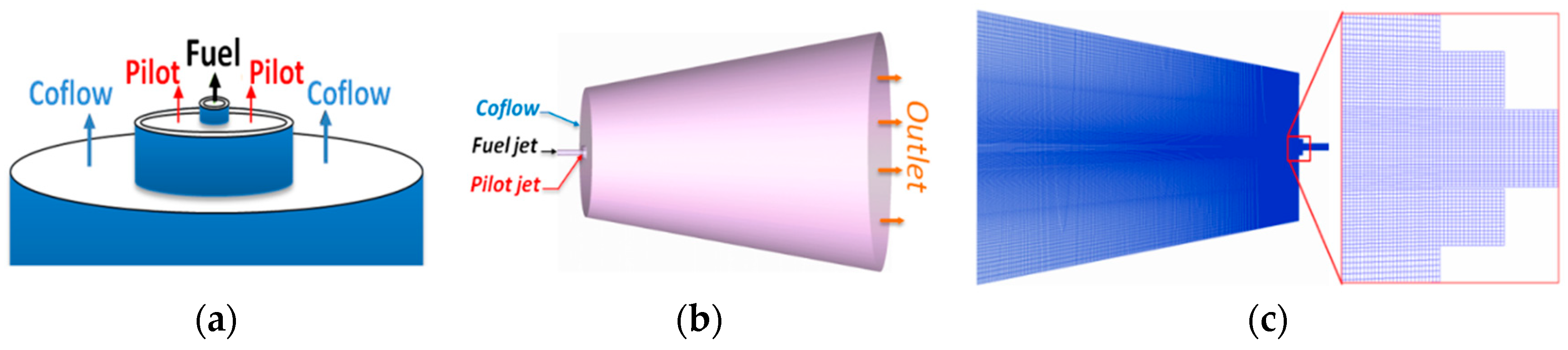
3.1. Air Piloted-Jet Flame (Sandia Flame D)

The burner geometry of the turbulent reacting configuration Sandia Flame-D [62] consists of a central fuel nozzle with diameter dfuel = 7.2 mm (the wall thickness is 0.25 mm) surrounded by a pilot jet burner with dpilot = 18.2 mm (the wall thickness is 0.35 mm). The main jet is constituted by a mixture of 25% methane and 75% air by volume. The pilot jet burns a premixture of acetylene (C2H2), hydrogen (H2), air, carbon dioxide (CO2), and nitrogen (N2). It is operated lean. This configuration was planted in an air-wind tunnel around the nozzle presenting the coflow stream with diameter dcoflow = 165 mm. Based on the central fuel nozzle properties it exhibited a Reynolds number of 22,400. Various scalar data obtained from Raman/Rayleigh/LIF (Laser-Induced fluorescence) measurement techniques and velocity data from two-component LDV measurements are available [62]. Figure 2 features the computational configuration studied where a 3D structured grid with 40 blocks and 1,808,440 control volumes has been found sufficient to accomplish grid-insensitive solutions. The height of the numerical grid applied was 80 dfuel. Regarding the numerical set-up, the waveTransmissive condition was used for the outlet with fixed pressure value; P = 1 atm, and zero gradient boundary conditions were set for all other parameters. All the operating conditions are provided in Table 1. To assess the convergence of the number of stochastic fields (SFi), the LES was carried out for different numbers of stochastic fields (4,6,8,16 SFi) for 0.38 s of physical time, respectively, to ensure that the flow reaches the statistically steady state with time step Δt = 3 × 10⁻⁷. The calculations were accomplished on 96 processors.

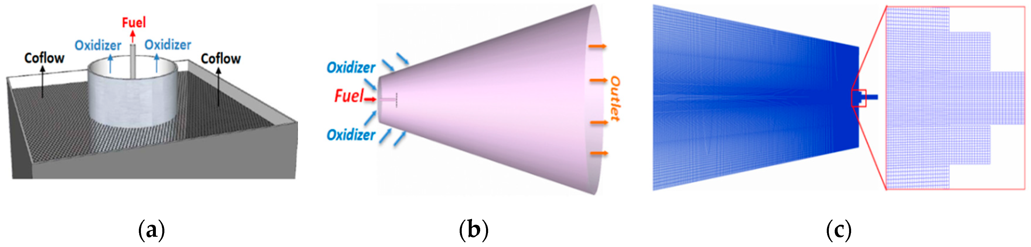
3.2. Oxy-Fuel Jet Flame (Flame B3)

The oxy-fuel jet flame B3 is one of the flame series that were experimentally studied in [43]. It exhibits a Reynolds number Re = 18,000, making it interesting for LES investigations. The reacting turbulent burner is composed mainly of two jets; a central jet with an inner diameter dB3-fuel = 5 mm (the wall thickness is 0.5 mm) for the fuel stream with a mixture of 55% H2 and 45% CH4, and a coaxially arranged jet with diameter dB3-oxy = 96.5 mm for the premixed oxidizer composition of 68% CO2 and 32% O2. In fact, it has been reported in [63,64], that air flame stability is established once the O2% content is around 30% which explains the specie percentages used for the oxidizer stream in this study. Further, the existence of H2 in the fuel jet helps the flame to remain attached to the nozzle as indicated in [43]. Figure 3 presents the 3D configuration of flame B3 featuring the computational domain in a conical shape assuming that the base and the sides are inlets for the oxidizer, which helps the numerical convergence of the calculations. The block-structured hexahedral grid applied consists of 89 blocks and 2,800,770 cells in an O-ring arrangement. 8450 cells are used for the fuel pipe jet, with minimum cell size equal to 5.31 × 10⁻¹² m3 and maximum cell size located in the outlet region with 1.09 × 10⁻¹⁰ m3. To assess the LES quality, various criteria are available, as reported in [46,47,48,49,50,51,52,53,54,55,56,57,58,59,60,61,62,63,64,65]. In the present paper we adopt the approach proposed by Hanjalic et al. in [66] and Pope in [7]. Thus, based on the ratio of the LES local mesh size Δ to the Kolmogorov length scale η , it turns out that Δ / η 12 in almost the entire computational domain, which reflects that more than 80% of the turbulent kinetic energy are resolved, along with the Taylor scales. Thereby, the Kolmogorov length scale, that has to be estimated by RANS solution following the procedure in [67], has been evaluated by RANS calculations from [4]. The outlet plane is at x = 80 dB3-fuel, with waveTransmissive condition and fixed pressure P = 1 atm. Similar to the previous case, zero gradient boundary conditions are imposed for other variables and the temperature is initially uniformly distributed. More details for the operating conditions are summarized in Table 2. To evaluate the convergence of the number of stochastic fields, SFi, calculations for different cases (using 4,8,16 SFi) were also run in this case, however on 160 processors for 0.16 s of physical time with time step Δt = 2.5 × 10⁻⁷. For the inlet turbulent flow field velocity of both studied cases, an in house turbulence inflow generator according to [68] was used.

4. Results

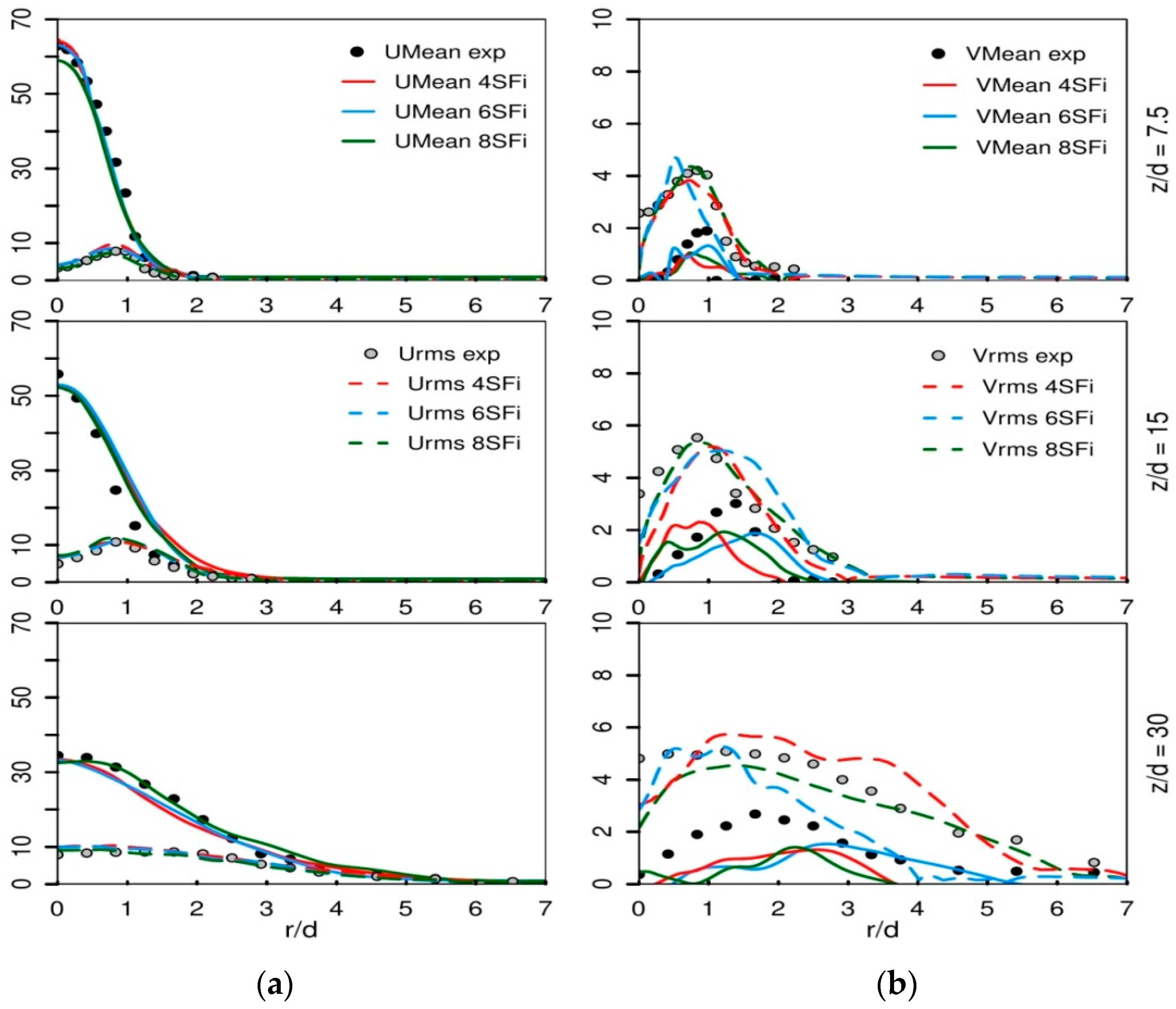
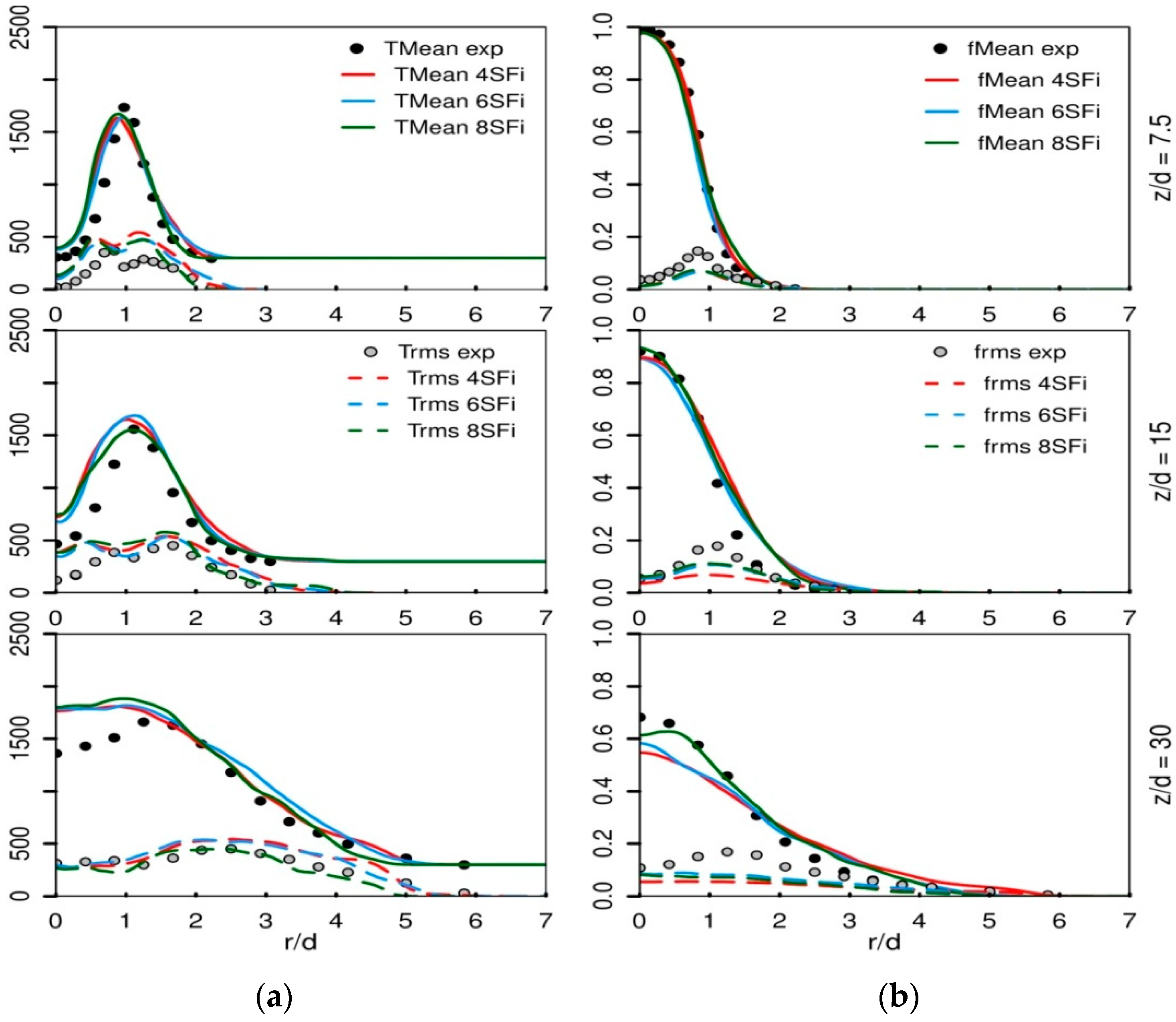
4.1. Validation on an Air-Piloted Jet Flame (Sandia Flame D)

In this section, the Sandia flame D is used to support the evaluation of the performance of the LES hybrid FESF/FPV. This is achieved in terms of comparison between numerically obtained results with experimental data for various radial profiles of some scalar quantities, scatter plots and probability density function at three axial positions, z/d = 7.5; 15 and 30. Thereby, different simulations using different numbers of Stochastic Fields (SFi = 4, 6, 8 and 16) are presented, in order to assess the convergence of the number of SFi. Time mean and root mean square (rms) of both axial and radial velocity are displayed in Figure 4. For the axial velocity, the obtained radial profile results feature a good overall agreement with experimental data at different positions for both mean (solid line) and rms quantities (dashed line). However, some under-estimations are noticed in reproducing the behavior of the radial velocity at z/d = 15 while an over-prediction is observed at z/d = 30. By applying various numbers of stochastic fields, it turns out that the mean quantities of the radial velocity obtained with 8SFi are predicted better at all axial positions.
Figure 5 depicts the radial profiles of temperature and mixture fraction at different axial positions. Regarding the mixture fraction evolution, numerical results indicate an excellent agreement for both mean and rms quantities at the axial position z/d = 7.5, and a slight under-estimation at the middle axial location further from the centerline without exhibiting any differences once using varied stochastic field numbers. However, the mean temperature at the centerline was slightly over-predicted at both positions z/d = 7.5 and 15 in Figure 5a, independently from the number of stochastic fields. This over-prediction was mostly pronounced at the centerline only at the further downstream positions, which is explained by the under-estimation of mixture fraction at same axial position. The influence of using different stochastic field numbers is revealed by comparing the rms quantities of the temperature. It appears clearly that the use of 8SFi allows for an overall better prediction. Such a SFi number agrees with that found by Jones et al. [31]. Further, the reported results proved the efficiency of the suggested novel method once compared to available measurements and to other previous numerical studies in which different flamelet models coupled to the FPV approach have been adopted. In fact, regarding the different computational setups employed in the case of Sandia Flame-D, Coclite et al. in [69] used the statistically most likely distribution model (SMLD) coupled to the FPV technique and found the mixture fraction profiles at different axial positions rather slightly under-predicted near the centerline. In [15], the mean temperature profiles were slightly over-predicted in some axial positions far from the centerline.
Figure 6 shows two series of instantaneous scatter plots of the temperature distribution at 3 axial positions. The first series exhibit the calculated instantaneous scatter plots plotted versus the instantaneous mixture fraction quantities, when 8 SFi are used (Figure 6, bottom). The second series present the reference instantaneous scatter plots (Figure 6, top). It turns out that the maximum temperature corresponding to the stochiometric mixture fraction is well predicted for all locations except the first axial position where it is very slightly overestimated with small deviations. Some local extinction values could not be predicted numerically in the region close to the centerline. However, one can note the presence of few unrealistic structures of temperature in the mixture fraction range 0.8 < f < 0.9 for both axial positions z/d = 7.5 and 15. This could shape up due to the standard mixing model used in this work. The Interaction by exchange of mean (IEM) is known, by nature, to be not local in composition space which may lead to unphysical events (see in [70]). As reported in [57] where two different mixing models (IEM and EMST (Euclidean minimum spanning tree)) have been tested on all piloted Sandia flames including the Flame-D, the IEM approach could not capture perfectly the conditional temperature distribution leading to a similar unphysical trend within the same mixture fraction range as observed also in [58].
Another quantity which is essential to evaluate numerical combustion models in predicting the flame characteristics is the probability density function (PDF). Figure 7 displays the PDF of the temperature at 2 axial locations further downstream from the flame nozzle obtained numerically using different SFi numbers in comparison with experimental data. This PDF was calculated for a narrow band of the mixture fraction around the stoichiometry where 0.30 < f < 0.40. The PDFs obtained calculated using 8 SFi are showing better results comparing to other numerical results simulated with less fields, where very similar behavior to the available experimental data is illustrated. In particular, the probability of the presence of temperature ranging from 1650 K to 2150 K is comparable to the measurements at both positions, z/d = 15 and 30. Next, the novel LES hybrid ESF/FPV model was applied to investigate the evolution of oxy-fuel flame characteristics.

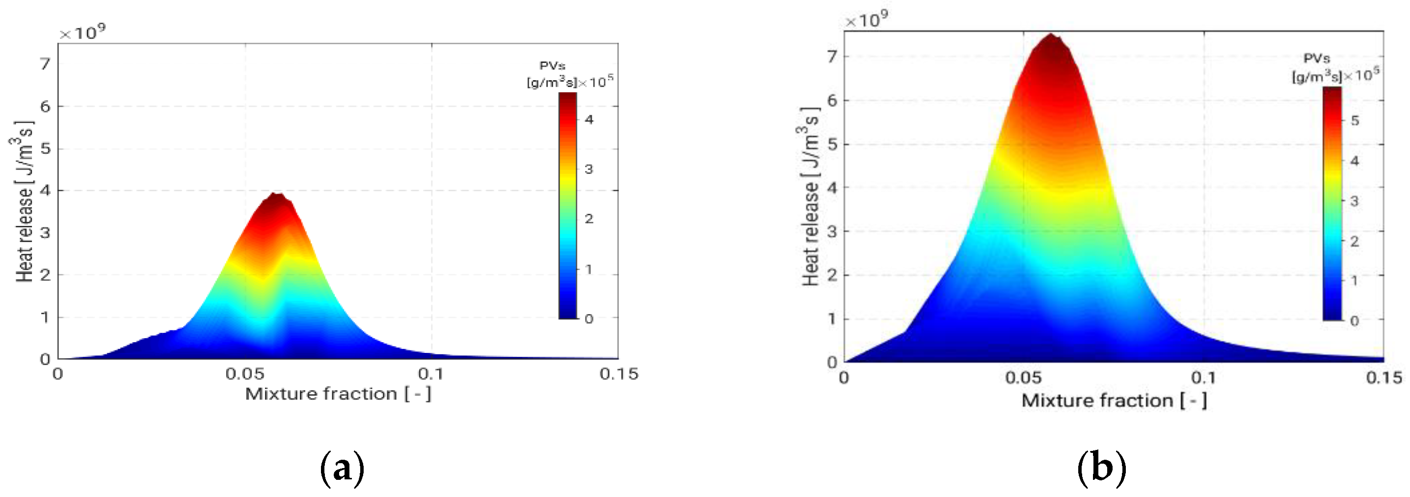
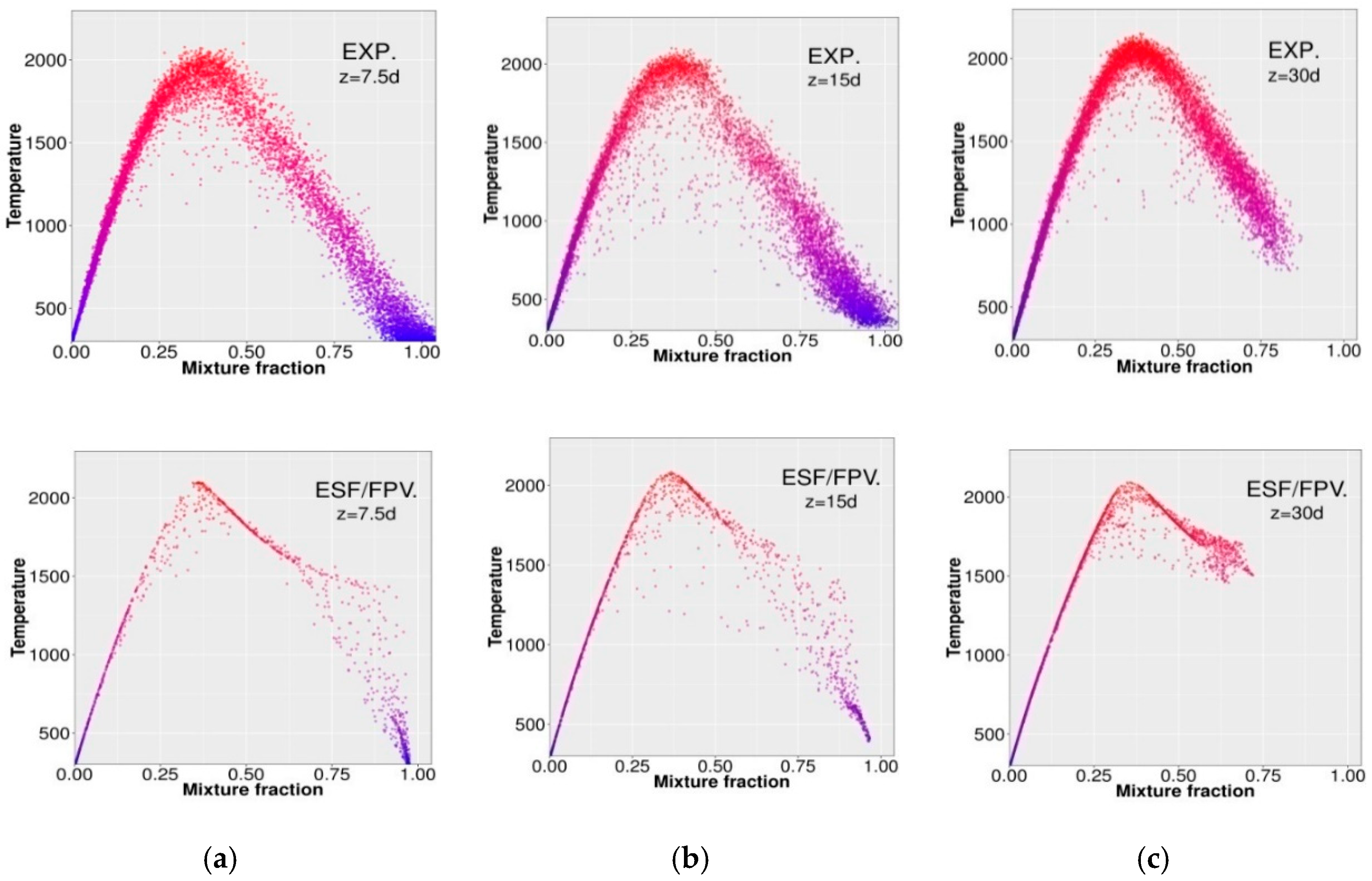
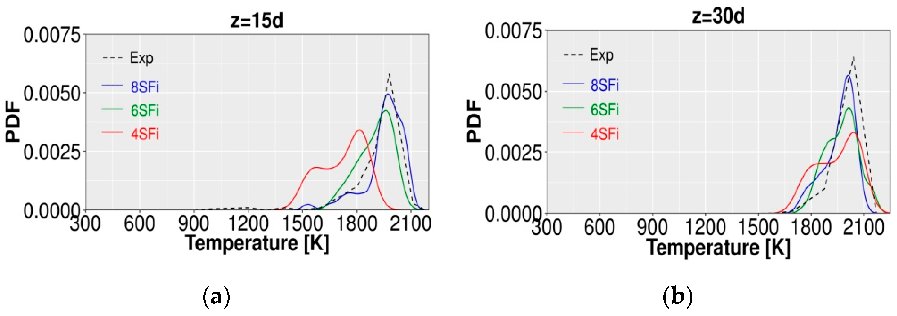
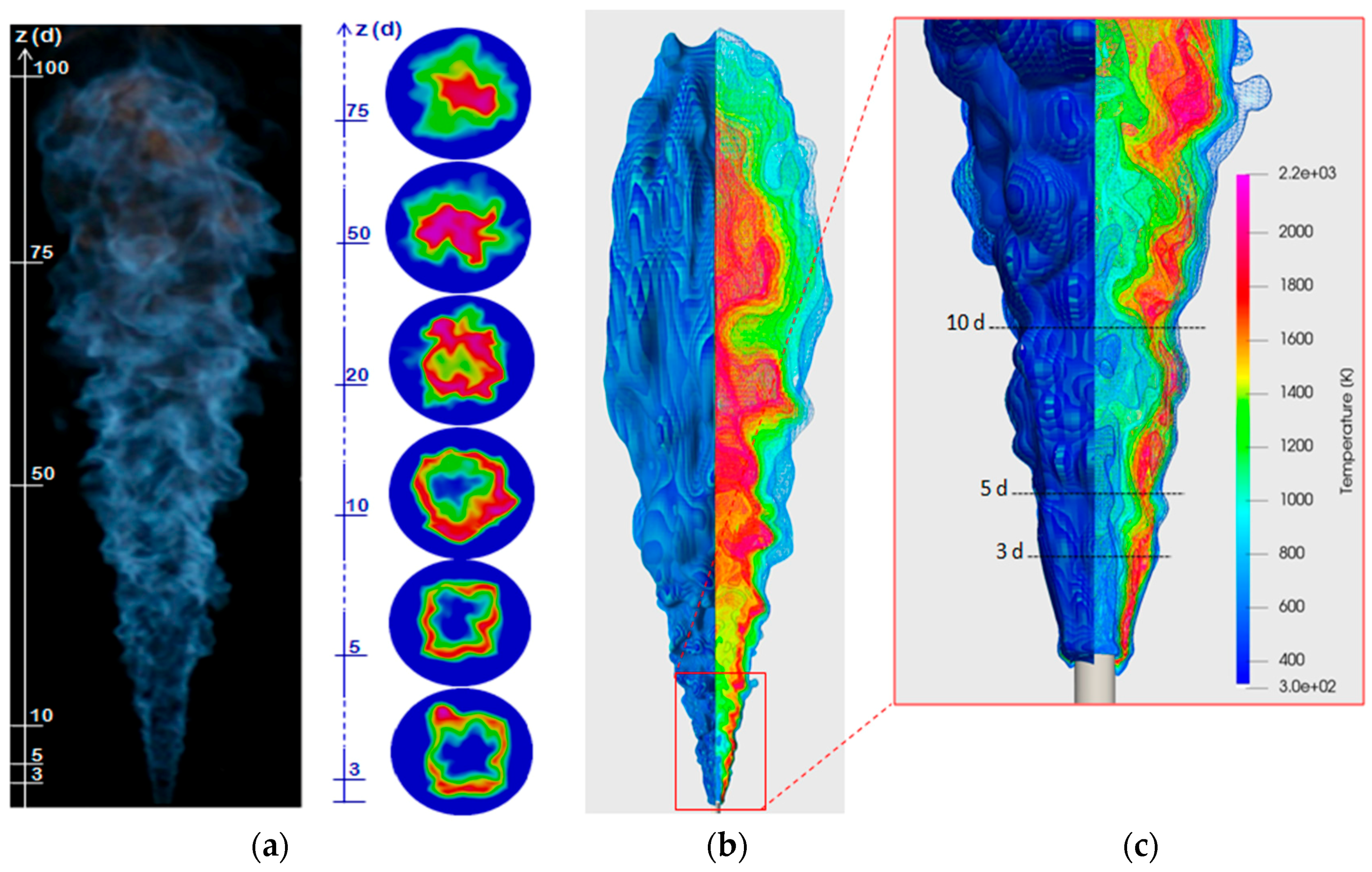
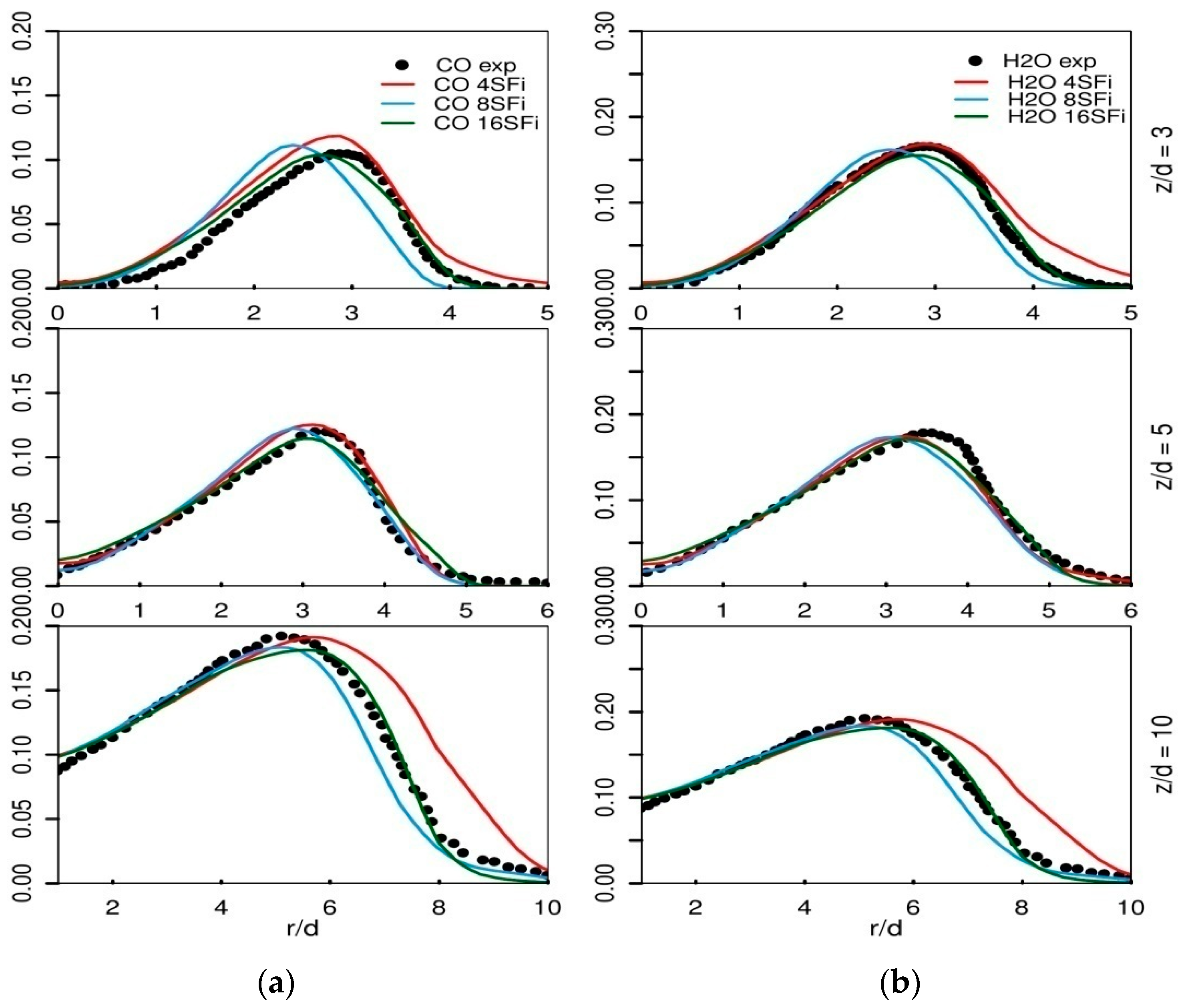
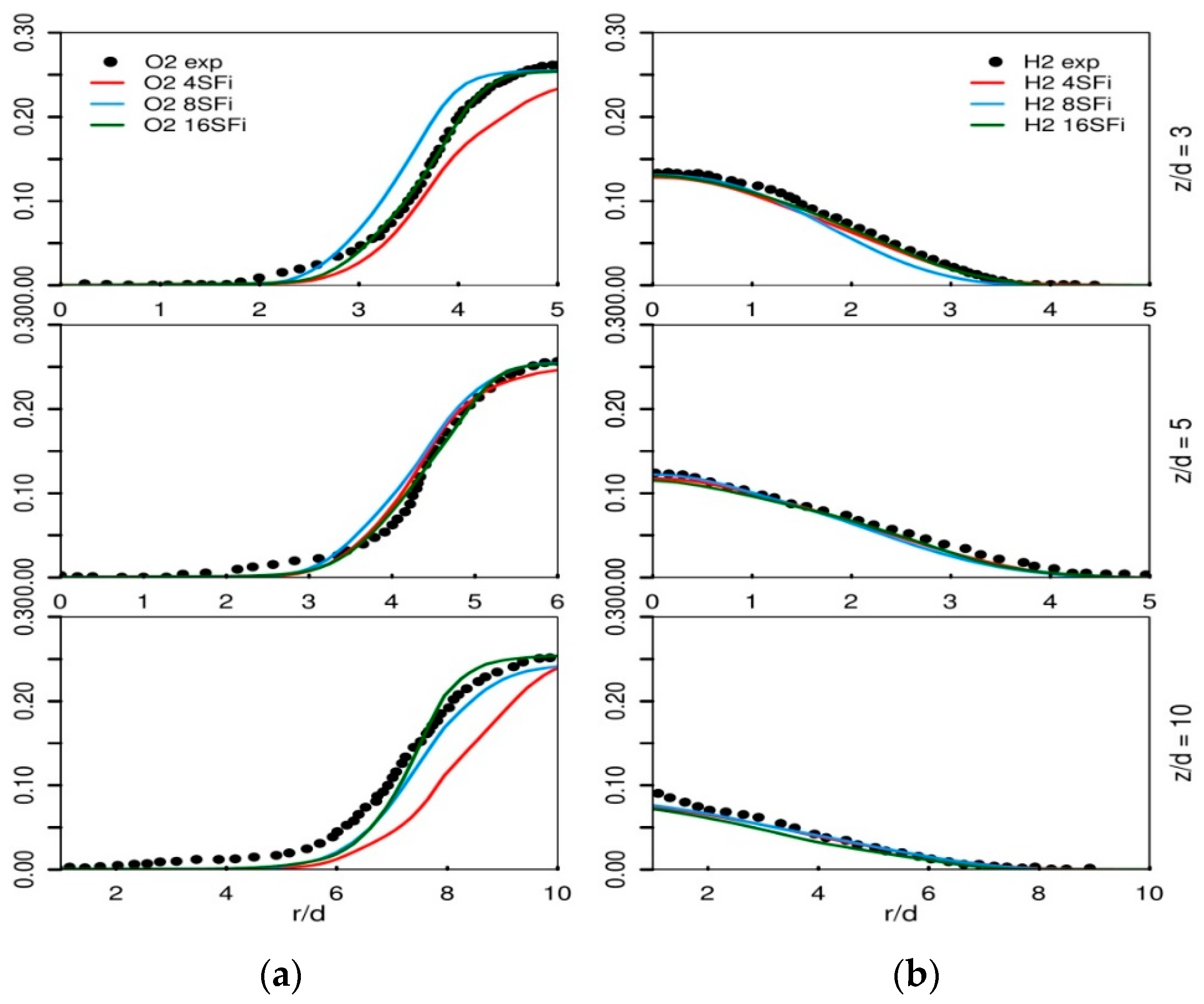
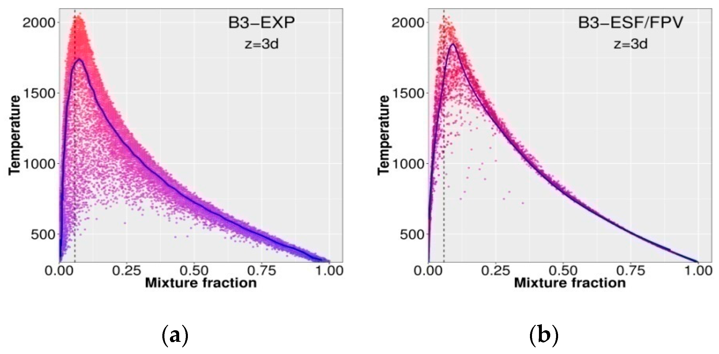
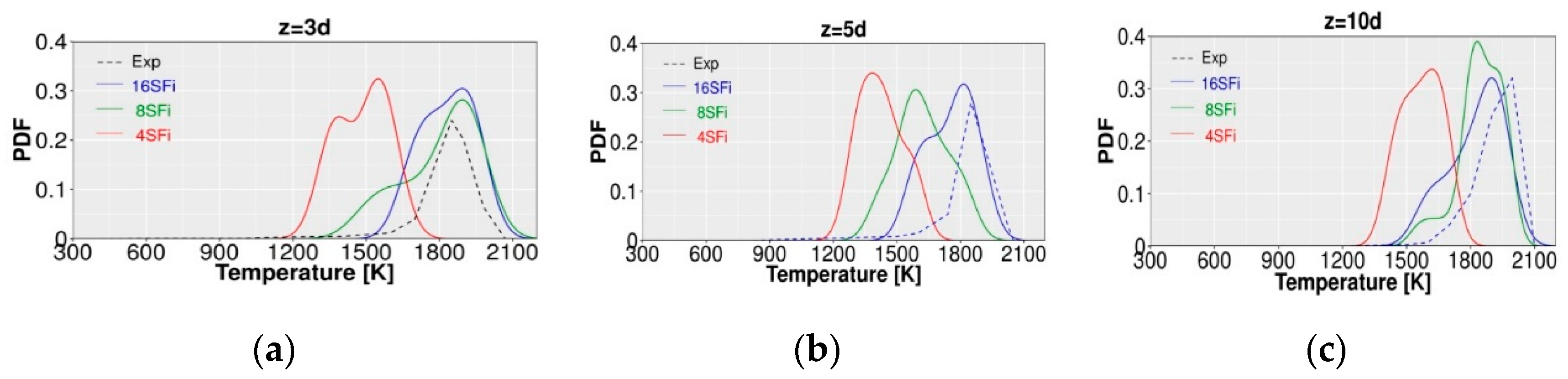
4.2. Application to Oxy-Fuel Jet Flame B3

The LES hybrid ESF/FPV was now appraised on the oxy-flame B3 in terms of comparison with available measurements, and then applied to analyze the effect of CO2 dilution on the oxy-flame behavior. First, Figure 8 shows qualitatively both experimental and numerical instantaneous temperature field for oxy-flame B3. Thereby, the region close to the nozzle of the burner is particularly zoomed in order to clearly display the measurement planes. The predicted flame length observed in Figure 8c agrees reasonably well with the experimental data, which reached approximately Lflame = 100 dB3-fuel (see in Figure 8a).
Figure 8b shows the instantaneous temperature contour on radial planes at different axial positions; it can be seen that the temperature field spreads radially and toward the outlet of the burner. The flame is also shown attached to the burner nozzle as it is observed experimentally under consideration of the important amount of diluted H2 in the fuel mixture. In the zoomed region above the fuel nozzle (Figure 8c right), the temperature field reaches the maximum predicted value, which corresponds to 2250 K found in experiments.
The quantitative validation was achieved by comparisons with experimental data in Figure 9, Figure 10, Figure 11 and Figure 12 of the evolution of main species and temperature, as well as of the scatter plots and probability density function of scalars at different axial positions. To ensure the convergence of the number of stochastic fields (SFi) various simulations are performed by applying different numbers of Stochastic Fields (4, 8 and 16). Figure 9 shows the evolution of the mean values of CO and H2O species mass fractions at different axial positions. The amounts of CO and H2O mass fractions were much higher than values obtained with air diluted flame cases. Especially, close to the nozzle, the CO and H2O mass fractions were equal to 0.11 and 0.18, respectively. However, these values increased to almost 0.2 for both species at higher axial positions. In this way, the present LES results confirm the RANS-based findings of Rihab et al. in [4], which agree with Masri et al. in [71], who reported that the CO2 68% diluted with pure oxygen in the oxidizer inlet is not inert. This plays an important role in increasing CO and H2O gases formation since the additional CO2 reacts with H to form CO. Figure 10 presents the mean quantities of O2 and H2 species mass fractions. In both figures, the results with 16 SFi achieved better agreements at radial profiles once compared to results with 4 SFi. This is not surprising, since four stochastic fields are not sufficient to reproduce the exact evolution of measured quantities (see also previous case: Sandia flame-D results using 4SFi).
In general, the results of CO and H2O mass fraction at axial positions close to the nozzle using 8 SFi are shifted in Figure 9 toward the axial centerline. Further downstream, the agreement with experimental data is excellent. Similar observations can be made in Figure 10 for the results of O2 and H2 species mass fractions with 8 SFi. While slight under-prediction of O2 at z/d = 10 was recorded, the use of different SFi numbers had a negligibly small impact on the H2 mass fraction evolution.
The instantaneous scatter plots of the temperature distribution at axial position near the fuel nozzle (z/d = 3) were compared with available experimental data in Figure 11. Thereby, the vertical black line drawed in both plots corresponds to the stochiometric mixture fraction value. The maximum reached value of the temperature distribution was 2100 K, which matches the experimental data. All values referring to the extinction locations were properly reproduced numerically. However, the lowest value predicted with the simulation reads 750 K, while experimentally it is 500 K. Furthermore, the mean temperature profile is lightly overestimated near the stoichiometry region comparing to experimental results.
Figure 12 compares the PDF calculated using different numbers of SFi with those obtained from measurements at axial positions z/d = 3; 5 and 10. For both sets, the PDF was estimated for a narrow band of the mixture fraction around the stoichiometry where ∆ = 0.04. In most locations, the shape of the PDF of the temperature could be reproduced only with simulation results using 16 SFi, but slight differences were noticed at both last axial positions where few values of temperature in the range of 1500 K and 1700 K were over-predicted numerically. Nevertheless, the probability of the presence of the temperature range from 1800 K to 2100 K is matching the values obtained experimentally for all positions in a good way.

5. Conclusions

In this paper, it was demonstrated that the combustion characteristics of a turbulent oxy-methane non-premixed flame operating under highly diluted conditions of CO2 and H2 in oxidizer and fuel streams, respectively, can be predicted and analyzed using a novel hybrid ESF/FPV model designed for that purpose. It combines a transported joint scalar probability density function (T-PDF) following the Eulerian stochastic field methodology (ESF), and a flamelet progress variable (FPV) turbulent combustion model under consideration of a detailed chemical reaction mechanism. This novel hybrid ESF/FPV approach removes the weaknesses of the presumed-probability density function (P-PDF)-based FPV modeling along with the solving of associated additional modeled transport equations while rendering the T-PDF computationally less affordable.
The prediction capability of the LES hybrid ESF/FPV was first appraised successfully on an air- piloted methane jet flame (Sandia Flame D). Then, it was assessed in analyzing the combustion properties of an oxy-flame, the so-called oxy-flame B3 under investigation and in capturing CO2 effect on the behavior of the oxy-flame. These configurations were previously investigated by the authors using a RANS-based formulation of this model. Relying on the results achieved, the following conclusions can be listed:
  • Overall, the LES hybrid filtered ESF/FPV approach demonstrated its high capability in capturing the main flame characteristics and flow field variables not only in the Sandia flame D but also in an oxy-flame configuration with CO2 and H2 dilution in oxidizer and fuel streams, respectively, using FPV tables based on Le = 1. This indicates that the H2 induced differential diffusion effect is not important in the investigated area of this oxy-flame B3.
  • Compared to our RANS results in our previous work [4], the LES hybrid ESF/FPV model provides more accurate predictions.
  • A good convergence of the optimal number of stochastic fields (SFi) strongly depends on the complexity of the combustion case. Even though more SFi could help to achieve fully complete convergence in this regard, in search of saving computational costs it turned out that a simulation with at least 8 stochastic fields leads to an accurate prediction in Sandia flame D as in [31] and at least 16 stochastic fields allow achieving better results in accordance with measurements once complex configuration like the oxy-fuel flame-B3 is investigated.
  • Regarding the general prediction of the oxy-flame structure, stability and emissions, it turns out that 68% molar percentage of additional CO2 enrichment in the oxidizer side leads to 0.39% of CO formation near the burner fuel nozzle and 0.62% at 10 dfuel above the nozzle. These amounts of CO-formed gases are clearly high compared to ordinary flame cases with air/fuel conditions with 0.35% near the burner nozzle and 0.62% at 10 dfuel above the jet tip.
The novel model needs to be further evaluated by using FPV tables with a non-unity Lewis number and by considering advanced micro-mixing models coupled to the LES hybrid ESF/FPV approach. All of these tasks are left for future work.

Author Contributions

Conceptualization, R.M., and A.S.; Methodology, R.M., M.J. and A.S.; T-PDF solver, M.J.; Hybrid-ESF/FPV solver development, R.M., M.J. and A.S.; Settings up, R.M.; Simulations and Validation, R.M. Formal Analysis, R.M., and AS.; Investigation, R.M.; Resources, A.S., B.F. and J.J.; Data Curation, R.M.; Writing-Original Draft Preparation, R.M.; Writing-Review & Editing, A.S., M.J., F.R. and B.F.; Visualization, A.S.; Supervision, A.S. and B.F.; Project Administration, A.S.

Funding

This project was funded by the European Union’s Horizon 2020 under the Marie Sklodowska-Curie grant agreement 643134 (CLEAN-Gas).

Acknowledgments

The authors of this work gratefully acknowledge the financial support by the European Union’s Horizon 2020 research and innovation program [CLEAN-Gas] with grant number 643,134, also the financial support by the DFG (German Research Council) CRC/Transregio 150 Turbulent, chemically reactive, multi-phase flows near walls. All the numerical simulations were carried out on the Hessen High Performance Computer (HHLR) at the Technical University of Darmstadt.

Conflicts of Interest

The authors declare no conflict of interest.

Nomenclature

C s Model constant
C ɸ Micro-mixing model coefficient
dW Wiener term
fMixture fraction
F Joint probability density function
G Filter function
N Number of stochastic field
N α Number of the chemical table controlling variables
p Pressure
P Probability density function
Re Reynolds number
S ij Strain rate tensor
t Time
T Temperature
u i Velocity component in ith direction
W Molar mass
x i Positions coordinate in ith direction
Y Mass fraction
Δ t Time increment
δ ij Kronecker-symbol
ρ Density
μ Dynamic molecular viscosity
μ t Dynamic turbulent viscosity
σ Schmidt number
σ sgs Sub-grid turbulent Schmidt number
ω ˙ Chemical source term
ɸ General species variable
δ Dirac delta function
ψ Composition space of species
α Referring to table controlling variable
ξ α n nth stochastic field of the variable α
( . ) ˜ Favre weighted quantity
( . ) ¯ Mean quantity
Lflame Length of the flame
dfuelDiameter of the fuel Nozzle of Sandia Flame-D
dpilotDiameter of the pilot Nozzle of Sandia Flame-D
dcoflowDiameter of the coflow of Sandia Flame-D
dB3-fuelDiameter of the fuel Nozzle of Oxy-flame B3
dB3-oxyDiameter of the pilot Nozzle of Oxy-flame B3
T-PDFTransported probability density function
ESFEulerian Stochastic Field
PVProgress Variable
FPVFlamelet Progress Variable
P-PDFPresumed probability density function
SDEStochastic differential equations
LESLarge Eddy Simulation
CCSCarbon Capture and Storage
FGMFlamelet Generated Manifold
CMCConditional Moment Closure

References

  1. Emission Database for Global Atmospheric research EDGAR, European Commission. Available online: http://edgar.jrc.ec.europa.eu/overview.php?v=CO2andGHG1970-2016 (accessed on 26 March 2019).
  2. Leunga, D.Y.C.; Caramannab, G.; Mercedes, M.V.M. An overview of current status of carbon dioxidecapture and storage technologies. Renew. Sustain. Energy Rev. 2014, 39, 426–443. [Google Scholar] [CrossRef]
  3. White, V.; Torrente-Murciano, L.; Sturgeon, D.; Chadwick, D. Purification of Oxyfuel-derived CO2. In Proceedings of the 9th International Conference on Greenhouse Gas Control Technologies, Washington DC, USA, 16–20 November 2008; Volume 2, pp. 399–406. [Google Scholar]
  4. Mahmoud, R.; Jangi, M.; Fiorina, B.; Pfitzner, M.; Sadiki, A. Numerical Investigation of an Oxyfuel non-premixed combustion using a Hybrid Eulerian Stochastic Field/Flamelet Progress Variable approach: Effects of H2/CO2 enrichment and Reynolds number. Energies 2018, 11, 3158. [Google Scholar] [CrossRef]
  5. Sadiki, A.; Janicka, J. Large Eddy Simulation of Turbulent Combustion Systems. Proc. Combust. Inst. 2005, 30, 537–547. [Google Scholar] [CrossRef]
  6. Smagorinsky, J. General circulation experiments with the primitive equations. Basic Exp. Mon. Weather Rev. 1963, 91, 99–164. [Google Scholar] [CrossRef]
  7. Pope, S.B. Turbulent Flows, 2nd ed.; Cambridge University Press: Cambridge, UK, 2000. [Google Scholar]
  8. Pierce, C.D.; Moin, P. Progress-variable approach for large-eddy simulation of non-premixed turbulent combustion. J. Fluid Mech. 2004, 504, 73–97. [Google Scholar] [CrossRef]
  9. Fiorina, B.; Veynante, D.; Candel, S. Modeling Combustion Chemistry in Large Eddy Simulation of Turbulent Flames. Flow Turbul. Combust. 2015, 94, 3–42. [Google Scholar] [CrossRef]
  10. Maas, U.; Pope, S.B. Simplifying chemical kinetics: Intrinsic low-dimensional manifolds in composition space. Combust. Flame 1992, 88, 239–264. [Google Scholar] [CrossRef]
  11. Bykov, V.; Maas, U. The extension of the ILDM concept to reaction–Diffusion manifolds. Combust. Theory Model. 2007, 11, 839–862. [Google Scholar] [CrossRef]
  12. Van Oijen, J.A.; Donini, A.; Bastiaans, R.J.M.; Ten-Thije-Boonkkamp, J.H.M.; De-Goey, L.P.H. State-of-the-art in premixed combustion modeling using flamelet generated manifolds. Science 2016, 57, 30–74. [Google Scholar] [CrossRef]
  13. Vicquel, R. Tabulated Chemistry for Turbulent Combustion Modelingand Simulation. Ph.D. Thesis, Laboratoire d’Énergétique Moléculaire et Macroscopique, Combustion (EM2C) du CNRS et de l’ECP, Ecole centrale Paris, Paris, France, June 2010. [Google Scholar]
  14. Ribert, G.; Domingo, P.; Vervisch, L. Hybrid transported-tabulated strategy to downsize detailed chemistry for Large Eddy Simulation. In Proceedings of the Center for Turbulence Research Proceedings of the Summer Program 2012, Stanford, CA, USA, 24 June–20 July 2012. [Google Scholar]
  15. Di Renzo, M.; Coclite, A.; De Tullio, M.D.; De Palma, P.; Pascazio, G. LES of the Sandia Flame D Using an FPV Combustion Model. In Proceedings of the 70th Conference of the ATI Engineering Association, Energy Procedia, Spienza University of Rome, Rome, Italy, 9–11 September 2015; pp. 402–449. [Google Scholar]
  16. Ihme, M.; Pitsch, H. Prediction of extinction and reignition in non-premixed turbulent flames using a flamelet/progress variable model: 2. Application in LES of Sandia flames D and E. Combust. Flame 2008, 15, 90–107. [Google Scholar] [CrossRef]
  17. Gierth, S.; Hunger, F.; Popp, S.; Wu, H.; Ihme, M.; Hasse, C. Assessment of differential diffusion effects in flamelet modeling of oxy-fuel flames. Combust. Flame 2018, 197, 134–144. [Google Scholar] [CrossRef]
  18. Ihme, M.; Pitsch, H. Prediction of extinction and reignition in non-premixed turbulent flames using a flamelet/progress variable model: 1. A priori study and presumed PDF closure. Combust. Flame 2008, 155, 70–89. [Google Scholar] [CrossRef]
  19. Mayer, B.; Prieler, R.; Demuth, M.; Moderer, L.; Hochneauer, C. CFD modelling and performance increase of a pusher type reheating furnace using oxy-fuel burners Bernhard. Energy Proc. 2017, 120, 462–468. [Google Scholar] [CrossRef]
  20. Prieler, R.; Mayr, B.; Demuth, M.; Spoljaric, D.; Hochenauer, C. Application of the steady flamelet model on a lab-scale and an industrial furnace for different oxygen concentrations. Energy 2015, 91, 451–464. [Google Scholar] [CrossRef]
  21. Mayer, B.; Prieler, R.; Demuth, M.; Hochneauer, C. The usability and limits of the steady flamelet approach in oxy-fuel combustions. Energy 2015, 90, 1478–1489. [Google Scholar] [CrossRef]
  22. Hidouri, A.; Chrigui, M.; Boushaki, T.; Sadiki, A.; Janicka, J. Large eddy simulation of two isothermal and reacting turbulent separated oxy-fuel jets. Fuel 2017, 192, 108–120. [Google Scholar] [CrossRef]
  23. Kuhne, J.; Ketelheun, A.; Janicka, J. Analysis of sub-grid PDF of progress variable approach using a hybrid LES/TPDF method. Proc. Combust. Inst. 2011, 33, 1411–1418. [Google Scholar] [CrossRef]
  24. Kim, G.; Kim, Y.; Joo, Y.J. Conditional Moment Closure for Modeling Combustion Processes and Structure of Oxy-Natural Gas Flame. Energy Fuels 2009, 23, 4370–4377. [Google Scholar] [CrossRef]
  25. Garmory, A.; Mastorakos, E. Numerical simulation of oxy-fuel jet flames using unstructured LES-CMC. Proc. Combust. Inst. 2014, 35, 1207–1214. [Google Scholar] [CrossRef]
  26. El-Asrag, H.; Graham, G. A comparison between two different Flamelet reduced order manifolds for non-premixed turbulent flames. In Proceedings of the Laminar Turbulent Flames 8th U.S. National Combustion Meeting, Park City, UT, USA, 19–22 May 2013. [Google Scholar]
  27. Pope, S.B. PDF methods for turbulent reactive flows. Prog. Energy Combust. 1985, 11, 119–192. [Google Scholar] [CrossRef]
  28. Mejia, J.M.; Sadiki, A.; Molina, A.; Chejne, F.; Pantangi, P. Large Eddy Simulation of the Mixing of a Passive Scalar in a High-Schmidt Turbulent Jet. J. Fluids Eng. 2015, 137, 31301–31311. [Google Scholar] [CrossRef]
  29. Mejia, J.M.; Chejne, F.; Molina, A.; Sadiki, A. Scalar Mixing Study at High-Schmidt Regime in a Turbulent Jet Flow Using Large-Eddy Simulation/Filtered Density Function Approach. J. Fluids Eng. 2016, 138, 021205. [Google Scholar] [CrossRef]
  30. Raman, V.; Pitsch, H.; Fox, R. Eulerian transported probability density function sub-filter model for LES simulations of turbulent combustion. Combust. Theory Model. 2007, 10, 439–458. [Google Scholar] [CrossRef]
  31. Jones, W.P.; Prasad, V.N. Large Eddy Simulation of the Sandia Flame Series (D, E and F) using the Eulerian stochastic field method. Combust. Flame 2010, 157, 1621–1636. [Google Scholar] [CrossRef]
  32. Jones, W.P.; Marquis, A.; Prasad, V. LES of a turbulent premixed swirl burner using the Eulerian stochastic field method. Combst. Flame 2012, 159, 3079–3095. [Google Scholar] [CrossRef]
  33. Avdic, A.; Kuenne, G.; DiMare, F.; Janicka, J. LES combustion modeling using the Eulerian stochastic field method coupled with tabulated chemistry. Combust. Flame 2017, 175, 201–219. [Google Scholar] [CrossRef]
  34. Jangi, M.; Li, C. Modelling of Methanol Combustion in a Direct Injection Compression Ignition Engine using an Accelerated Stochastic Fields Method. Energy Procedia 2017, 105, 1326–1331. [Google Scholar] [CrossRef]
  35. Valińo, L. A field Monte Carlo formulation for calculating the probability density functions of a single scalar in turbulent flow. Flow Turbul. Combust. 1998, 60, 157–172. [Google Scholar] [CrossRef]
  36. Sabelnikov, V.; Soulard, O. Rapidally decorrelating velocity-field model as tool for solving one-point Fokker-Planck equations for probability density functions of turbulent reactive scalars. Phys. Rev. 2005, 72. [Google Scholar] [CrossRef]
  37. Mustata, R.; Valińo, L.; Jimenez, C.; Jones, W.; Bondi, S. A probability density function Eulerian Monte Carlo method for large eddy simulations: Application to a turbulent piloted methane/air diffusion flame (Sandia-D). Combust. Flame 2006, 145, 88–104. [Google Scholar] [CrossRef]
  38. Jangi, M.; Zhao, M.; Haworth, D.C.; Bai, X.S. Stabilization and liftoff length of a non-premixed methane/air jet flame discharging into a high-temperature environment: An accelerated transported PDF method. Combust. Flame 2015, 162, 408–419. [Google Scholar] [CrossRef]
  39. Gong, C.; Jangi, M.; Bai, X.S.; Liang, J.H.; Sun, M.B. Large eddy simulation of hydrogen combustion in supersonic flows using an Eulerian stochastic fields method. Int. J. Hydrogen Energy 2017, 42, 1264–1275. [Google Scholar] [CrossRef]
  40. Prasad, V.N.; Luo, K.H.; Jones, W.P. LES-PDF Simulation of a highly sheared turbulent piloted premixed flame. In Proceedings of the 7th Mediterranean Combustion Symposium, Sardinia, Italy, 11–15 September 2011; pp. 1–12. [Google Scholar]
  41. Girimaji, S.S. Assumed β-pdf Model for Turbulent Mixing: Validation and Extension to Multiple Scalar Mixing. Combust. Sci. Technol. 2007, 78, 177–196. [Google Scholar] [CrossRef]
  42. Garmory, A.; Richardson, E.; Mastorakos, E. Micro-mixing effects in a reacting plume by the stochastic field method. Aton. Environ. 2006, 40, 1078–1091. [Google Scholar] [CrossRef]
  43. Sevault, A.; Dunn, M.; Barlow, R.S.; Ditaranto, M. On the Structure of the Near Field of Oxy-Fuel Jet Flames Using Raman/Rayleigh Laser Diagnostics. Conbust. Flame 2012, 159, 3342–3352. [Google Scholar] [CrossRef]
  44. Ditaranto, M.; Sautet, J.C.; Samaniego, J.M. Structural aspects of coaxial oxy-fuel flames. Exp. Fluids 2001, 30, 253–261. [Google Scholar] [CrossRef]
  45. Favre, A. Equations des gaz turbulents compressibles, 2, Méthodes des vitesses moyennes; méthode des vitesses macroscopiques pondérées par la masse volumique. J. Mech. 1965, 4, 392–421. [Google Scholar]
  46. Ries, F.; Nishad, K.; Dressler, L.; Janicka, J.; Sadiki, A. Evaluating large eddy simulation results based on error analysis. Theor. Comput. Fluid Dyn. 2018, 32, 733–752. [Google Scholar] [CrossRef]
  47. Driest, V. On Turbulent Flow near a Wall. J. Aeronaut. Sci. 1956, 23, 1007–1011. [Google Scholar] [CrossRef]
  48. Deardorff, J.W. A numerical study of three-dimensional turbulent channel flow at large Reynolds numbers. J. Fluid Mech. 1970, 41, 453–480. [Google Scholar] [CrossRef]
  49. Kempf, A.; Sadiki, A.; Janicka, J. Prediction of finite chemistry effects using large eddy simulation. Proc. Combust. Inst. 2003, 29, 1979–1985. [Google Scholar] [CrossRef]
  50. FlameMaster v3.3.10. Available online: https://web.stanford.edu/group/pitsch/FlameMaster.htm (accessed on 26 March 2019).
  51. Gri-Mesh3.0. Available online: http://www.me.berkeley.edu/gri_mech/ (accessed on 26 March 2019).
  52. Ihme, M.; Shunn, L.; Zhang, J. Regularization of reaction progress variable for application to flamelet-based combustion models. J. Comput. Phys. 2012, 231, 7715–7721. [Google Scholar] [CrossRef]
  53. Pope, S.B. A Monte Carlo Method for the PDF Equations of Turbulent Reactive Flow. J. Combust. Sci. Technol. 2008, 25, 159–174. [Google Scholar] [CrossRef]
  54. Jones, W.P.; Martinez, S.N. Numerical Study of n-heptane auto-ignition using LES-PDF methods. Flow Turbul. Combust. 2009, 83, 407–423. [Google Scholar] [CrossRef]
  55. Gao, F.; O’Brien, E.E. A large-eddy simulation scheme for turbulent reacting flows. AIP Phys. Fluids 1993, 5, 1282–1284. [Google Scholar] [CrossRef]
  56. Dopazo, C. Probability density function approach for a turbulent axisymmetric heated jet. Centerline evolution. Phys. Fluids 1975, 18, 397–404. [Google Scholar] [CrossRef]
  57. Jaishree, J.; Haworth, D.C. Comparisons of Lagrangian and Eulerian PDF methods in simulations of non-premixed turbulent jet flames with moderate-to-strong turbulence-chemistry interactions. Combust. Theory Model. 2012, 16, 435–463. [Google Scholar] [CrossRef]
  58. Hinz, A. Numerische Simulation Turbulenter Methan-Diffusionsflammen Mittels Monte Carlo PDF Methoden. Ph.D. Thesis, Energy and Power Plant Technology, Mechanical Department, Technical University of Darmstadt, Darmstadt, Germany, April 2000. [Google Scholar]
  59. Gardiner, C.W. Handbook of Stochastic Methods for Physics, Chemistry and the Natural Sciences; Springer: Berlin/Heidelberg, Germany, 2009. [Google Scholar]
  60. Greenshields, C.J. OpenFOAM Programmer’s Guide; OpenFOAM Foundation Ltd.: London, UK, 2009. [Google Scholar]
  61. Schneider, C.; Dreizler, A.; Janicka, J.; Hassel, E. Flow field measurements of stable and locally extinguishing hydrocarbon-fuelled jet flames. Combust. Flame 2003, 135, 185–190. [Google Scholar] [CrossRef]
  62. TNF Workshop. Available online: http://www.ca.sandia.gov/TNF (accessed on 26 March 2019).
  63. Ditaranto, M.; Hals, J. Combustion instabilities in sudden expansion oxy–fuel flames. Combust. Flame 2006, 146, 493–512. [Google Scholar] [CrossRef]
  64. Coppens, F.H.V.; Konnov, A.A. The effects of enrichment by H2 on propagation speeds in adiabatic flat and cellular premixed flames of CH4 + O2 + CO2. Fuel 2008, 81, 2866–2870. [Google Scholar] [CrossRef]
  65. Doost, A.S.; Ries, F.; Becker, L.G.; Burkle, S.; Wagner, S.; Ebert, V.; Dreizler, A.; di Mare, F.; Sadiki, A.; Janicka, J. Residence time calculations for complex swirling flow in a combustion chamber using large-eddy simulations. Chem. Eng. Sci. 2016, 156, 97–114. [Google Scholar] [CrossRef]
  66. Hanjalic, K.; Popovac, M.; Hadziabdic, M. A robust near-wall elliptic-relaxation eddy-viscosity turbulence model for CFD. Int. J. Heat Fluid Flow 2004, 25, 1047–1051. [Google Scholar] [CrossRef]
  67. Hadziabdic, M.; Hanjalic, K. Vortical structures and heat transfer in a round impinging jet. J. Fluid Mech. 2008, 596, 221–260. [Google Scholar] [CrossRef]
  68. Klein, M.; Sadiki, A.; Janicka, J. A digital filter based generation of inflow data for spatially developing direct numerical or large eddy simulations. J. Comput. Phys. 2003, 186, 652–665. [Google Scholar] [CrossRef]
  69. Coclite, A.; Pascazio, G.; De Palma, P.; Cutrone, L.; Ihme, M. An SMLD Joint PDF Model for Turbulent Non-Premixed Combustion Using the Flamelet Progress-Variable Approach. Flow Turbul. Combust. 2015, 95, 97–119. [Google Scholar] [CrossRef]
  70. Subramaniam, S.; Pope, S. A mixing model for turbulent reactive flows based on Euclidean minimum spanning trees. Combust. Flame 1998, 115, 487–517. [Google Scholar] [CrossRef]
  71. Masri, A.R.; Dibble, R.W.; Barlow, R.S. Chemical kinetic effects in non-premixed flames of H2/CO2 fuel. Combust. Flame 1992, 91, 285–309. [Google Scholar] [CrossRef]
Figure 1. Distribution of production rate of heat release in the mixture fraction space colored with source term of the progress variable (PV): (a) Flame-D table, (b) Oxyflame B3 table.
Applsci 09 01320 g001
Figure 2. Sandia Flame-D burner, (a) Description of the experimental configuration, (b) The numerical configuration generated (c) 3D structured grid used with a zoom of the inlet nozzle region where smoother grid is applied.
Applsci 09 01320 g002
Figure 3. Flame B3 burner, (a) Description of the experimental configuration (b) The numerical configuration generated, (c) 3D structured grid used with a zoom on the fuel inlet nozzle region where smoother grid is applied.
Applsci 09 01320 g003
Figure 4. Comparison between experimental data for Sandia Flame-D and large eddy simulation (LES) hybrid Eulerian stochastic field (ESF)/flamelet progress variable (FPV) numerical results for different numbers of stochastic fields (SFi) at different axial positions, z/d = 7.5; 15 and 30. Radial profiles of mean and rms of (a) axial velocity, (b) radial velocity.
Applsci 09 01320 g004
Figure 5. Comparison between experimental data for Sandia Flame-D and LES hybrid ESF/FPV numerical results for different numbers of SFi at different axial positions, z/d = 7.5; 15 and 30. Radial profiles of mean and rms of (a) temperature (b) mixture fractio.
Applsci 09 01320 g005
Figure 6. Instantaneous scatter plots of temperature versus mixture fraction for different axial positions ((a) z/d = 0.75, (b) z/d = 15 and (c) z/d = 30). Comparison between experiment and simulation results; Top: Measurements; Bottom: LES hybrid FESF/FPV with 8 SFi.
Applsci 09 01320 g006
Figure 7. Probability density function of temperature within a mixture fraction range = 0.1 at different axial positions; z/d = 15 and 30. Comparison between experiment and simulation results; Solid lines: LES hybrid ESF/FPV results with different SFi numbers, Dashed line: Measurements.
Applsci 09 01320 g007
Figure 8. Instantaneous temperature field for the oxy-flame B3: (a) Measurements, (b) 2D contours on radial planes at different axial locations, (c) Left: 3D snapshot obtained with LES hybrid ESF/FPV. Right: A zoom of the region above the fuel nozzle.
Applsci 09 01320 g008
Figure 9. Comparison between experimental data for oxy-flame flame B3and LES hybrid ESF/FPV numerical results for different numbers of SFi at different axial positions; z/d = 3; 5 and 10. Radial profiles of mean mass (a) CO species, (b) H2O species.
Applsci 09 01320 g009
Figure 10. The figure was moved bellow the paragraph where it was mentioned for the first time, please confirm. Comparison between experimental data for oxy-flame flame B3 and LES hybrid ESF/FPV numerical results for different numbers of SFi at different axial positions; z/d = 3; 5 and 10. Radial profiles of mean mass fraction of (a) O2 species, (b) H2 species.
Applsci 09 01320 g010
Figure 11. Instantaneous scatter plots of temperature versus mixture fraction at the axial position z/d = 3. Comparison between experiment and simulation results; (a) Experimental data, (b) LES hybrid ESF/FPV with 16 SFi.
Applsci 09 01320 g011
Figure 12. Probability density function of temperature within a mixture fraction range = 0.04, at different axial positions (a) z/d = 3, (b) z/d = 5 and (c) z/d = 30. Comparison between experiment and simulation results; Solid line: LES hybrid ESF/FPV with different SFi numbers, Dashed line: Measurements.
Applsci 09 01320 g012
Table 1. Conditions for the piloted jet Flame-Sandia-D.
Flame JetfPVT (k)Ub (m/s)ν (m2/s)
Central jet0.156029449.61.513 × 10−5
Pilot jet0.0437188011.41.513 × 10−5
Coflow002910.91.513 × 10−5
Table 2. Conditions for the oxy-fuel jet Flame B3.
Flame JetfPVT (k)Ub (m/s)ν (m2/s)
Fuel jet10300117.83.271 × 10−5
Oxidizer jet00300 0.9333.271 × 10−5

