Analysis of Causal Relationships for Nutrient Removal of Activated Sludge Process Based on Structural Equation Modeling Approaches


Abstract
:
1. Introduction
2. Materials and Methods
2.1. Operational Data Acquisition
2.2. Structural Equation Model
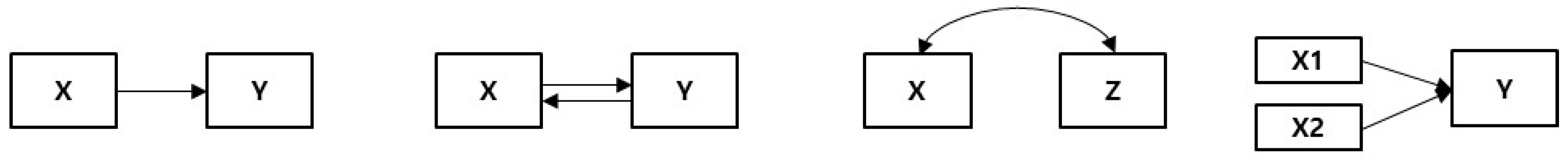
2.2.1. Path Model
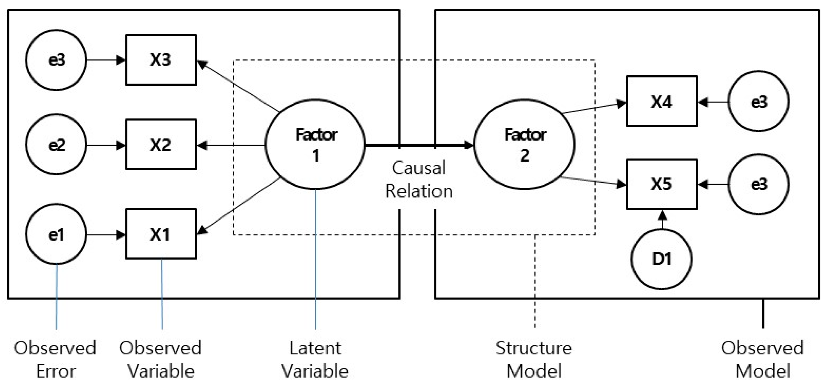
2.2.2. Structural Equation Model
3. Results
3.1. Structural Equation Modeling for Effluent T–N
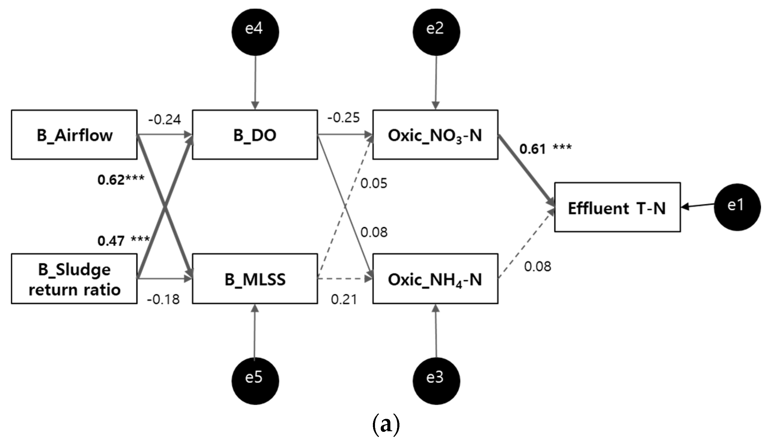
3.1.1. Path Model of Effluent T–N
Initial Path Model for Effluent T–N
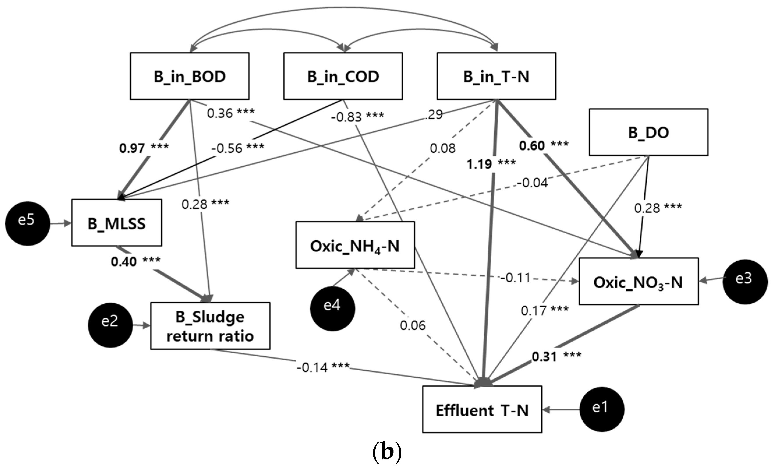
Modified path model for effluent T–N
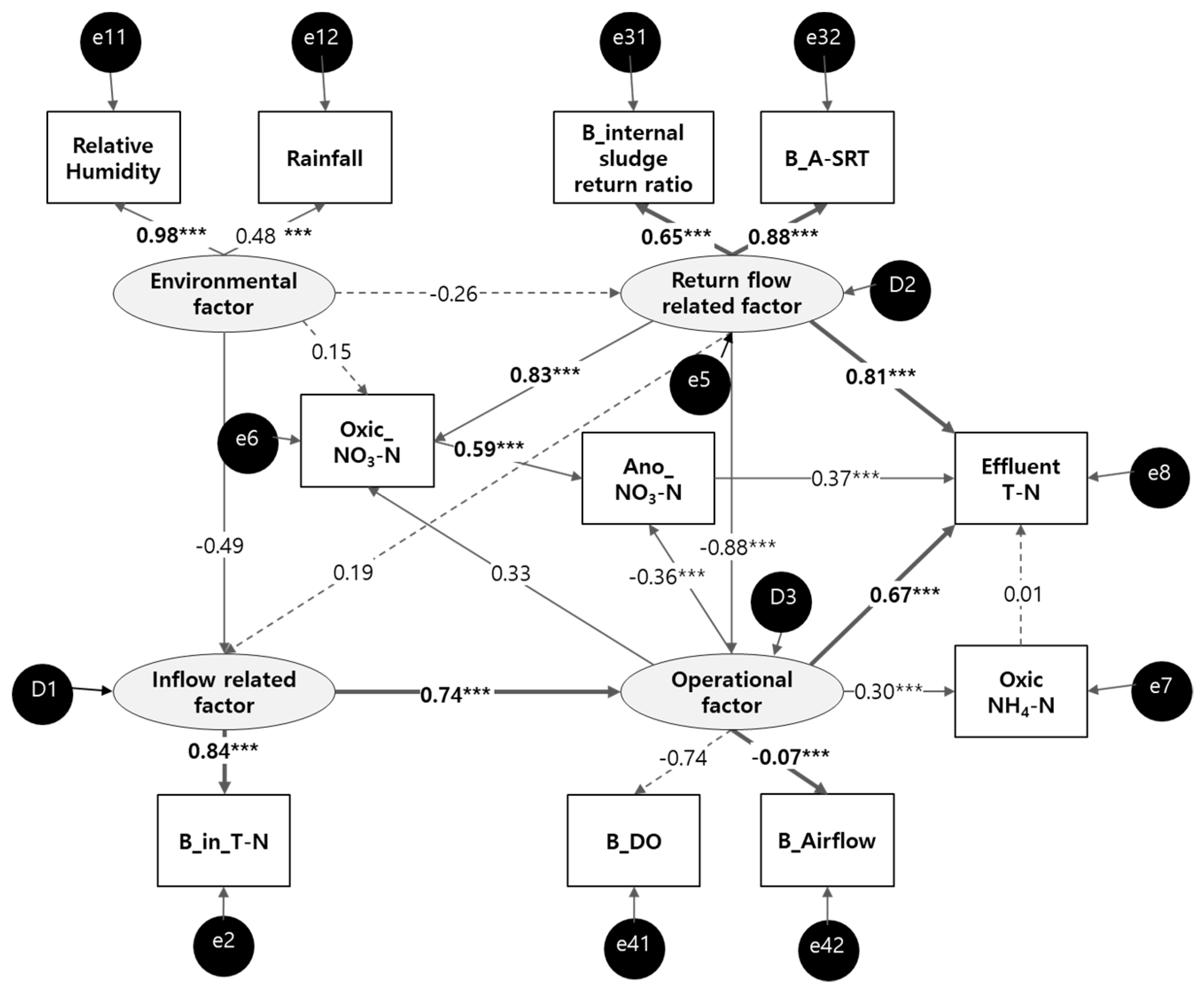
3.1.2. SEM for Effluent T–N
3.2. Structural Equation Modeling for Effluent T–P
3.2.1. Path Model of Effluent T–P
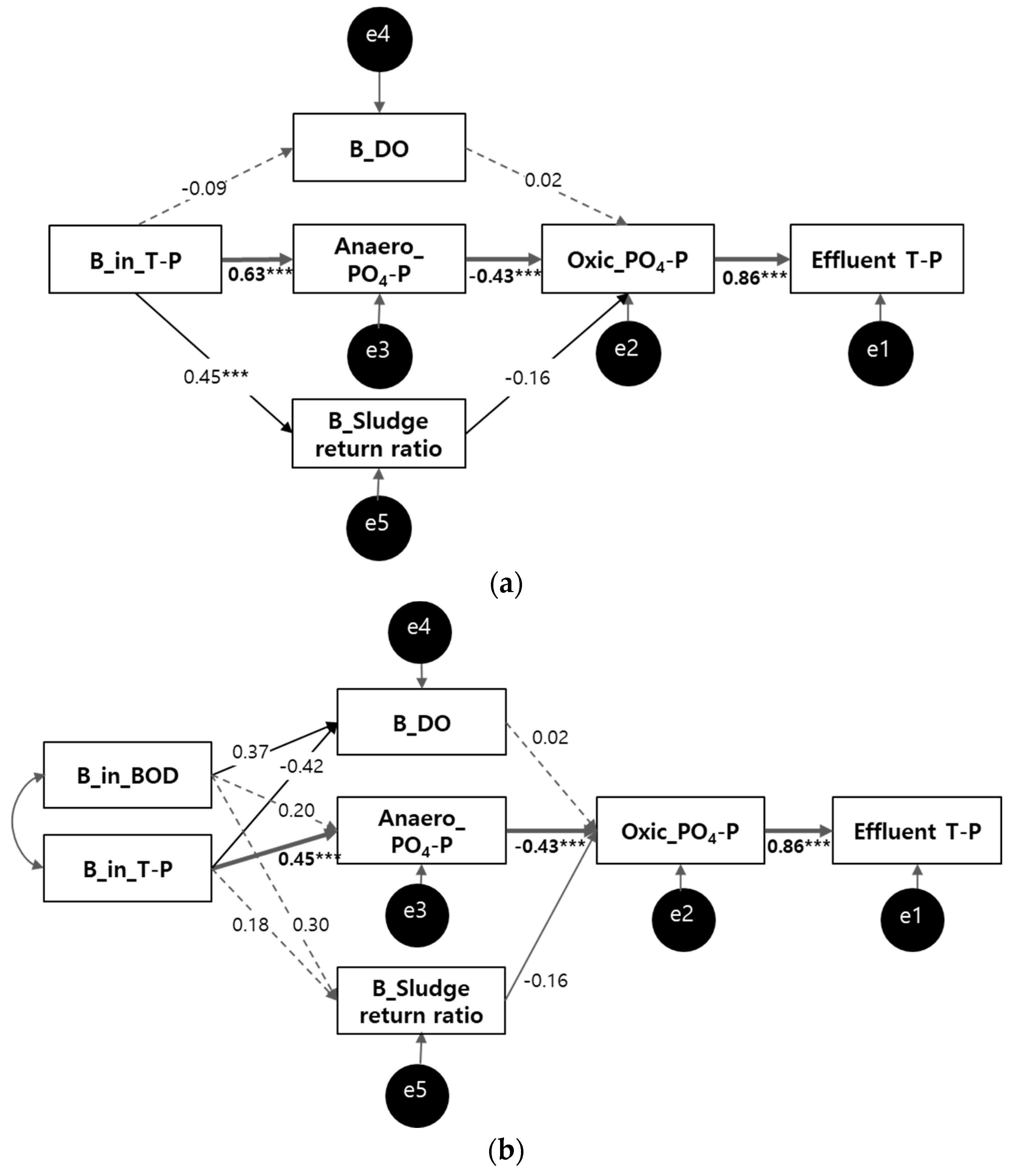
Initial Path Model for Effluent T–P
Modified Path Model for Effluent T–P
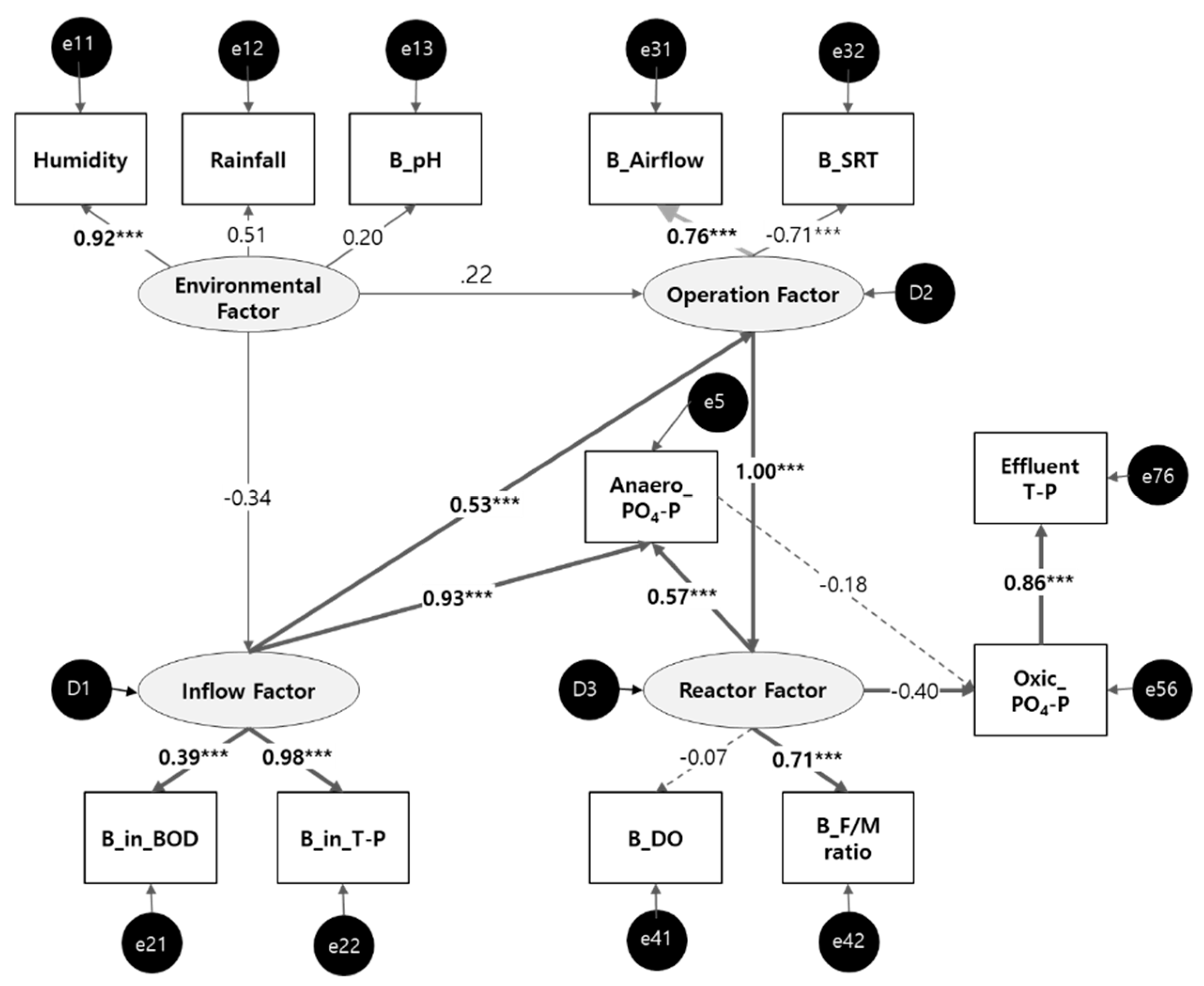
3.2.2. SEM for Effluent T–P
4. Discussion
5. Conclusions
Author Contributions
Funding
Conflicts of Interest
References
- Jenkins, D.; Wanner, J. Activated Sludge—100 Years and Counting; IWA Publishing: London, UK, 2014. [Google Scholar]
- Chong, H.G. Rule-based versus probabilistic approaches to the diagnosis of faults in wastewater treatment processes. Artif. Intell. Eng. 1996, 1, 265–273. [Google Scholar] [CrossRef]
- Rieger, L.; Gillot, S.; Langergraber, G.; Ohtsuki, T.; Shaw, A.; Takács, I.; Winkler, S. Chapter 5.4 Calibration and validation. In Guidelines for Using Activated Sludge Models; Scientific and Technical Report No. 22; IWA Publishing: London, UK, 2013. [Google Scholar]
- Cadet, C. Simplifications of Activated Sludge Model with preservation of its dynamic accuracy. IFAC Proc. Vol. 2014, 47, 7134–7139. [Google Scholar] [CrossRef]
- Müller, T.G.; Noykova, N.; Gyllenberg, M.; Timmer, J. Parameter identification in dynamical models of anaerobic waste water treatment. Math. Biosci. 2002, 177–178, 147–160. [Google Scholar] [CrossRef]
- Kim, H.W.; Lim, H.; Wie, J.; Lee, I.; Colosimo, M.F. Optimization of modified ABA2 process using linearized ASM2 for saving aeration energy. Chem. Eng. J. 2014, 251, 337–342. [Google Scholar] [CrossRef]
- Santa Cruz, J.A.; Mussati, S.F.; Scenna, N.J.; Gernaey, K.V.; Mussati, M.C. Reaction invariant-based of reduction of the activated sludge model ASM1 for batch applications. J. Environ. Chem. Eng. 2016, 4, 3654–3664. [Google Scholar] [CrossRef]
- Lee, J.M.; Yoo, C.; Choi, S.W.; Vanrolleghem, P.A.; Lee, I.B. Nonlinear process monitoring using kernel principal component analysis. Chem. Eng. Sci. 2004, 59, 223–234. [Google Scholar] [CrossRef]
- Lee, D.S.; Park, J.M.; Vanrolleghem, P.A. Adaptive multiscale principal component analysis for on-line monitoring of a sequencing batch reactor. J. Biotechnol. 2005, 116, 195–210. [Google Scholar] [CrossRef] [PubMed]
- Moon, T.S.; Kim, Y.J.; Kim, J.R.; Cha, J.H.; Kim, D.H.; Kim, C.W. Identification of process operating state with operational map in municipal wastewater treatment plant. J. Environ. Manag. 2009, 90, 772–778. [Google Scholar] [CrossRef] [PubMed]
- Wimberger, D.; Verde, C. Fault diagnosticability for an aerobic batch wastewater treatment process. Control Eng. Pract. 2008, 16, 1344–1353. [Google Scholar] [CrossRef]
- Baklouti, I.; Mansouri, M.; Hamida, A.B.; Nounou, H.; Nounou, M. Monitoring of wastewater treatment plants using improved univariate statistical technique. Process Saf. Environ. 2018, 116, 287–300. [Google Scholar] [CrossRef]
- Chow, C.W.K.; Liu, J.; Li, J.; Swain, N.; Reid, K.; Saint, C.P. Development of smart data analysis tools to support wastewater treatment plant operation. Chemom. Intell. Lab. Syst. 2018, 177, 140–150. [Google Scholar] [CrossRef]
- Cortés, U.; Martínez, M.; Comas, J.; Sánchez-Marré, M.; Poch, M.; Rodríguez-Roda, I. A conceptual model to facilitate knowledge sharing for bulking solving in wastewater treatment plants. AI Commun. 2003, 16, 279–289. [Google Scholar]
- Comas, J.; Rodríguez-Roda, I.; Sánchez-Marré, M.; Cortés, U.; Freixó, A.; Arrá, J.; Poch, M. A knowledge-based approach to the deflocculation problem: Integrating on-line, off-line, and heuristic information. Water Res. 2003, 37, 2377–2387. [Google Scholar] [CrossRef]
- Huang, Y.C.; Wang, X.Z. Application of fuzzy causal networks to waste water treatment plants. Chem. Eng. Sci. 1999, 54, 2731–2738. [Google Scholar] [CrossRef]
- Aulinas, M.; Nieves, J.C.; Cortés, U.; Poch, M. Supporting decision making in urban wastewater systems using a knowledge-based approach. Environ. Model. Softw. 2011, 26, 562–572. [Google Scholar] [CrossRef]
- Li, D.; Yang, H.Z.; Liang, X.F. Prediction analysis of a wastewater treatment system using a Bayesian network. Environ. Model. Softw. 2013, 40, 140–150. [Google Scholar] [CrossRef]
- Garvajal, G.; Roser, D.J.; Sisson, S.A.; Keegan, A.; Khan, S.J. Bayesian belief network modelling of chlorine disinfection for human pathogenic viruses in municipal wastewater. Water Res. 2017, 109, 144–154. [Google Scholar] [CrossRef]
- Grace, J.B. Structural Equation Modeling and Natural Systems; Cambridge University Press: Cambridge, UK, 2006. [Google Scholar]
- Arhonditsis, G.B.; Stow, C.A.; Steinberg, L.J.; Kenney, M.A.; Lathrop, R.C.; McBride, S.J.; Reekhow, K.H. Exploring ecological patterns with structural equation modeling and Bayesian analysis. Ecol. Model. 2006, 192, 385–409. [Google Scholar] [CrossRef]
- Grace, J.B.; Bollen, K.A. Representing general theoretical concepts in structural equation models; the role of composite variables. Environ. Ecol. Stat. 2008, 15, 191–213. [Google Scholar] [CrossRef]
- Grace, J.B.; Anderson, T.M.; Olff, H.; Scheiner, S.M. On the specification of structural equation models for ecological systems. Ecol. Monogr. 2010, 80, 67–87. [Google Scholar] [CrossRef] [Green Version]
- Grace, J.R.; Schoolmaster, D.R., Jr.; Guntenspergen, G.R.; Little, A.M.; Mitchell, B.R.; Miller, K.M.; Schweiger, E.W. Guidelines for a graph-theoretic implementation of structural equation modeling. Ecosphere 2012, 3, 1–44. [Google Scholar] [CrossRef]
- Capmourteres, V.; Anand, M. Assessing ecological integrity: A multi-scale structural and functional approach using Structural Equation Modeling. Ecol. Indic. 2016, 71, 258–269. [Google Scholar] [CrossRef]
- Pajunen, V.; Luoto, M.; Soininen, J. Unravelling direct and indirect effects of hierarchical factors driving microbial stream communities. J. Biogeogr. 2017, 44, 2376–2385. [Google Scholar] [CrossRef]
- Hatami, R. Development of a protocol for environmental impact studies using causal modeling. Water Res. 2018, 138, 206–223. [Google Scholar] [CrossRef]
- Villeneuve, B.; Valette, J.P.; Souchon, Y.; Usseglio-Polatera, P. Direct and indirect effects of multiple stressors on stream invertebrates across watershed, reach and site scales: A structural equation modelling better informing on hydromorphological impacts. Sci. Total Environ. 2018, 612, 660–671. [Google Scholar] [CrossRef] [PubMed]
- Sanches Fernandes, L.F.; Fernandes, A.C.P.; Ferreira, A.R.L.; Cortes, R.M.V.; Pacheco, F.A.L. A partial least squares—Path modeling analysis for the understanding of biodiversity loss in rural and urban watersheds in Portugal. Sci. Total Environ. 2018, 626, 1069–1085. [Google Scholar] [CrossRef] [PubMed]
- Zou, S.; Yu, Y.S. A general structural equation model for river water quality data. J. Hydrol. 1994, 162, 197–209. [Google Scholar] [CrossRef]
- Ariana, E.S.G.; Melissa, A.K.; Curtis, J.R. Examining the relationship between ecosystem structure and function using structural equation modelling: A case study examining denitrification potential in restored wetland soils. Ecol. Model. 2010, 221, 761–768. [Google Scholar] [CrossRef]
- He, J. Probabilistic Evaluation of Causal Relationship between Variables for Water Quality Management. J. Environ. Inform. 2016, 28, 110–119. [Google Scholar] [CrossRef]
- Zhu, L.; Zhou, H.; Xie, X.; Li, X.; Zhang, D.; Jia, L.; Wei, Q.; Zhao, Y.; Wei, Z.; Ma, Y. Effects of floodgates operation on nitrogen transformation in a lake based on structural equation modeling analysis. Sci. Total Environ. 2018, 631–632, 1311–1320. [Google Scholar] [CrossRef]
- Moreira, J.F.; Cabral, A.R.; Oliveira, R.; Silva, S.A. Causal model to describe the variation of faecal coliform concentrations in a pilot-scale test consisting of ponds aligned in series. Ecol. Eng. 2009, 35, 791–799. [Google Scholar] [CrossRef]
- Anderson, J.C.; Gerbing, D.W. Structural equation modeling in practice: A review and recommended two-step approach. Psychol. Bull. 1988, 103, 411. [Google Scholar] [CrossRef]
- Santibáñez-Andrade, G.; Castillo-Argüero, S.; Vega-Peña, E.V.; Lindig-Cisneros, R.; Zavala-Hurtado, J.A. Structural equation modeling as a tool to develop conservation strategies using environmental indicators: The case of the forests of the Magdalena river basin in Mexico City. Ecol. Indic. 2015, 54, 124–136. [Google Scholar] [CrossRef]
- Jöreskog, K.G.; Sörbom, D. LISREL VI: Analysis of Linear Structural Relationships by Maximum Likelihood and Least Square Methods; Scientific Software, Inc.: Mooresville, IN, USA, 1986. [Google Scholar]
- Jöreskog, K.G.; Sörbom, D. LISREL 8: User’s Reference Guide; Scientific Softwaer Internationa, Inc.: Chicago, IL, USA, 2001. [Google Scholar]
- Quinn, G.P.; Keough, M.J. Experimental Design and Data Analysis for Biologists; Cambridge University Press: New York, NY, USA, 2002. [Google Scholar]
- Wright, S. The method of path coefficient. Ann. Math. Stat. 1934, 5, 161–215. [Google Scholar] [CrossRef]
- Belkhiri, L.; Narany, T.S. Using Multivariate Statistical Analysis, Geostatistical Techniques and Structural Equation Modeling to Identify Spatial Variability of Groundwater Quality. Water Resour. Manag. 2015, 29, 2073–2089. [Google Scholar] [CrossRef]
- Hou, D.; Al-Tabbaa, A.; Chen, H.; Mamic, I. Factor analysis and structural equation modelling of sustainable behavior in contaminated land remediation. J. Clean. Prod. 2014, 84, 439–449. [Google Scholar] [CrossRef]
- Hair, J.F.J.; Anderson, R.E.; Tatham, R.L.; Black, W.C. Multivariate Data Analysis, 5th ed.; Prentice Hall: Upper Saddle River, NJ, USA, 1998. [Google Scholar]
- Hooper, D.; Coughlan, J.; Mullen, M. Structural equation modeling: Guidelines for determining model fit. Electron. J. Bus. Res. Methods 2008, 6, 53–60. [Google Scholar]
- Doll, W.J.; Xia, W.; Torkzadeh, G. A confirmatory factor analysis of the end-user computing satisfaction instrument. MIS Quart. 1994, 18, 357–369. [Google Scholar] [CrossRef]
- Baumgartner, H.; Homburg, C. Applications of Structural Equation Modeling in Marketing and Consumer Research: A review. Int. J. Res. Mark. 1996, 13, 139–161. [Google Scholar] [CrossRef]
- Ryberg, K.R. Structural equation model of total phosphorus loads in the Red River of the north basin, USA and Cananda. J. Environ. Qual. 2017, 46, 1072–1080. [Google Scholar] [CrossRef]
- Estiri, H. A structural equation model of energy consumption in the United States: Untangling the complexity of per-capita residential energy use. Energy Res. Soc. Sci. 2015, 6, 109–120. [Google Scholar] [CrossRef]
- Dang, H.L.; Li, E.; Nuberg, I.; Bruwer, J. Understanding farmer’s adaptation intention to climate change: A structural equation modelling study in the Mekong Delta, Vietnam. Environ. Sci. Policy 2014, 41, 11–22. [Google Scholar] [CrossRef]
- Wang, K.; Qiao, Y.; Li, H.; Zhang, H.; Yue, S.; Ji, X.; Liu, L. Structural equation model of the relationship between metals in contaminated soil and in earthworm (Metaphire californica) in Hunan Province, subtropical China. Ecotoxicol. Environ. Saf. 2018, 156, 443–451. [Google Scholar] [CrossRef] [PubMed]
- Ullman, J.B. Structural equation modeling: Reviewing the basics and moving forward. J. Personal. Assess. 2006, 87, 35–50. [Google Scholar] [CrossRef] [PubMed]
- Bagozzi, R.P.; Yi, Y. Specification, evaluation and interpretation of structural equation models. J. Acad. Mark. Sci. 2012, 40, 8–34. [Google Scholar] [CrossRef]


| Items | Variables |
|---|---|
| Weather conditions | Air temperature (°C), rainfall (mm), relative humidity (%) |
| Primary settling tank * | Water temperature (°C), pH, BOD (mg/L), COD (mg/L), SS (mg/L), T–N (mg/L), T–P (mg/L), alkalinity, S-BOD, HRT (h) |
| Bioreactor ** | Flow (m3/d), water temperature (°C), pH, DO (mg/L), MLSS (mg/L), MLVSS (mg/L), SVI, sludge return ratio (m3/d), Sludge return ratio (%), F/M ratio, BOD loading (kg/m3·day), SRT (day), A-SRT (day), Internal sludge-return ratio (%), ORP (mV), PO4–P (mg/L, at both anaerobic and anoxic tanks), NH4–N (mg/L, at both anoxic and oxic tanks), NO3–N (mg/L, at both anoxic and oxic tanks), air flow (m3/day), reactor volume (m3), HRT (h) |
| Effluent | Water temperature (°C), pH, BOD (mg/L), COD (mg/L), SS (mg/L), T–N (mg/L), T–P (mg/L), alkalinity, HRT (h) |
| Index | Acceptance Level | Classification |
|---|---|---|
| Q value | <3: Excellent | Parsimony-fit indices |
| Goodness of Fit Index (GFI) | >0.9: Excellent | Absolute-fit indices |
| Root Mean Square Error of Approximation (RMSEA) | <0.05: Excellent <0.08: Good <0.1: Normal | Absolute-fit indices |
| Adjusted Goodness of Fit Index (AGFI) | >0.8: Good | Absolute-fit indices |
| CFI | >0.9: Excellent | Incremental-fit indices |
| Classification | Goodness-of-Fit Criterion | Initial Model | Modified Model | ||
|---|---|---|---|---|---|
| Result | Validation | Result | Validation | ||
| Q value | below 3 | 2.303 (Fitness) | 1.373 (Fitness) | 1.652 (Fitness) | 2.111 (Fitness) |
| GFI | above 0.9 | 0.991 (Fitness) | 0.976 (Fitness) | 0.967 (Fitness) | 0.958 (Fitness) |
| AGFI | above 0.8 | 0.945 (Fitness) | 0.938 (Fitness) | 0.907 (Fitness) | 0.881 (Fitness) |
| RMSEA | below 0.05 (below 0.1) | 0.089 (Fitness) | 0.047 (Fitness) | 0.063 (Fitness) | 0.082 (Fitness) |
| CFI | above 0.9 | 0.983 (Fitness) | 0.979 (Fitness) | 0.989 (Fitness) | 0.980 (Fitness) |
| Variable | Component No. | |||
|---|---|---|---|---|
| 1 | 2 | 3 | 4 | |
| Rainfall | 0.038 | −0.652 | −0.232 | 0.253 |
| Relative humidity | −0.114 | −0.796 | −0.046 | −0.137 |
| B_pH | −0.154 | −0.758 | −0.136 | −0.126 |
| B_in_BOD | 0.858 | 0.278 | 0.006 | 0.103 |
| B_in_COD | 0.933 | 0.214 | 0.118 | 0.047 |
| B_in_SS | 0.874 | −0.192 | −0.103 | −0.065 |
| B_in_TN | 0.725 | 0.490 | 0.177 | 0.254 |
| B_in_TP | 0.869 | 0.401 | 0.116 | 0.021 |
| B_Sludge return ratio | 0.293 | 0.790 | 0.011 | 0.026 |
| B_internal sludge return ratio | 0.365 | 0.650 | 0.449 | 0.134 |
| B_A-SRT | 0.229 | 0.794 | 0.241 | 0.255 |
| B_SRT | 0.163 | 0.880 | 0.127 | 0.078 |
| B_Air flow | 0.069 | 0.102 | −0.704 | -0.044 |
| B_DO | −0.190 | −0.139 | 0.639 | 0.027 |
| B_MLSS | 0.325 | −0.456 | 0.565 | 0.226 |
| B_SVI | 0.262 | −0.450 | 0.551 | 0.370 |
| B_F/M ratio | 0.000 | −0.085 | −0.690 | −0.064 |
| Effluent_T-N | 0.333 | 0.268 | 0.266 | 0.610 |
| Factor | Variables |
|---|---|
| Environmental | Rainfall, relative humidity, B_pH |
| Inflow-related | B_in_BOD, B_in_COD, B_in_SS, B_in_T–N, B_in_T–P |
| Return flow-related | B_Sludge return ratio, B_Internal sludge-return ratio, B_A-SRT, B_SRT |
| Operational | B_Air flow, B_DO, B_MLSS, B_SVI, B_F/M ratio |
| Factor | Criterion | Result (Test) | Result (Validation) | Fitness/Not |
|---|---|---|---|---|
| Q value | <3 | 2.455 | 2.604 | Fitness |
| GFI | >0.9 | 0.924 | 0.919 | Fitness |
| AGFI | >0.8 | 0.847 | 0.838 | Fitness |
| RMSEA | <0.05 (<0.1) | 0.094 | 0.098 | Fitness |
| CFI | > 0.9 | 0.917 | 0.912 | Fitness |
| Classification | Goodness-of-Fit Criterion | Initial Model | Modified Model | ||
|---|---|---|---|---|---|
| Result | Validation | Result | Validation | ||
| Q value | below 3 | 1.263 (Fitness) | 1.659 (Fitness) | 1.902 (Fitness) | 1.949 (Fitness) |
| GFI | above 0.9 | 0.981 (Fitness) | 0.974 (Fitness) | 0.969 (Fitness) | 0.967 (Fitness) |
| AGFI | above 0.8 | 0.949 (Fitness) | 0.931 (Fitness) | 0.913 (Fitness) | 0.908 (Fitness) |
| RMSEA | below 0.05(below 0.1) | 0.040 (Fitness) | 0.063 (Fitness) | 0.074 (Fitness) | 0.076 (Fitness) |
| CFI | above 0.9 | 0.995 (Fitness) | 0.981 (Fitness) | 0.987 (Fitness) | 0.982 (Fitness) |
| Variable | Component No. | ||||
|---|---|---|---|---|---|
| 1 | 2 | 3 | 4 | 5 | |
| Rainfall | 0.083 | −0.508 | −0.176 | −0.111 | 0.548 |
| Relative humidity | −0.093 | −0.797 | −0.107 | −0.055 | 0.079 |
| B_pH | −0.106 | −0.680 | -0.009 | −0.252 | −0.370 |
| B_in_BOD | 0.845 | 0.313 | 0.006 | 0.118 | −0.023 |
| B_in_COD | 0.920 | 0.226 | 0.105 | 0.133 | -0.077 |
| B_in_SS | 0.893 | −0.134 | −0.070 | −0.116 | 0.082 |
| B_in_TN | 0.685 | 0.489 | 0.119 | 0.365 | −0.111 |
| B_in_TP | 0.852 | 0.401 | 0.118 | 0.110 | −0.138 |
| B_Sludge return ratio | 0.292 | 0.827 | 0.143 | −0.174 | −0.021 |
| B_internal sludge return ratio | 0.346 | 0.628 | 0.479 | 0.179 | −0.101 |
| B_A-SRT | 0.191 | 0.216 | 0.696 | 0.494 | −0.052 |
| B_SRT | 0.132 | 0.059 | 0.779 | 0.409 | −0.167 |
| B_Air flow | 0.031 | 0.078 | −0.807 | 0.131 | −0.211 |
| B_DO | −0.156 | 0.058 | 0.131 | 0.115 | 0.791 |
| B_MLSS | 0.296 | 0.643 | -0.442 | 0.094 | 0.060 |
| B_SVI | 0.253 | 0.272 | −0.367 | 0.026 | 0.677 |
| B_F/M ratio | −0.010 | −0.043 | −0.006 | −0.107 | −0.715 |
| Effluent_T-P | 0.087 | −0.220 | 0.291 | 0.751 | −0.093 |
| Factor | Variables |
|---|---|
| Environmental | Rainfall, relative humidity, B_pH |
| Inflow-related | B_in_BOD, B_in_COD, B_in_SS, B_in_T–N, B_in_T–P |
| Operational | B_Air flow, B_MLSS, B_Sludge return ratio, B_Internal sludge return ratio, B_A-SRT, B_SRT |
| Reactor-related. | B_DO, B_SVI, B_F/M ratio |
| Factor | Criterion | Result (Test) | Result (Validation) |
|---|---|---|---|
| Q value | <3 | 2.892 (Fitness) | 3.439 (Not fitness) |
| GFI | >0.9 | 0.883 (Not Fitness) | 0.861 (Not fitness) |
| AGFI | >0.8 | 0.810 (Fitness) | 0.775 (Not fitness) |
| RMSEA | <0.05 (<0.1) | 0.107 (Not Fitness, but close) | 0.121 (Not fitness) |
| CFI | >0.9 | 0.911 (Fitness) | 0.854 (Not fitness) |
© 2019 by the authors. Licensee MDPI, Basel, Switzerland. This article is an open access article distributed under the terms and conditions of the Creative Commons Attribution (CC BY) license (http://creativecommons.org/licenses/by/4.0/).
Share and Cite
Kim, Y.; Lee, S.; Cho, Y.; Kim, M. Analysis of Causal Relationships for Nutrient Removal of Activated Sludge Process Based on Structural Equation Modeling Approaches. Appl. Sci. 2019, 9, 1398. https://0-doi-org.brum.beds.ac.uk/10.3390/app9071398
Kim Y, Lee S, Cho Y, Kim M. Analysis of Causal Relationships for Nutrient Removal of Activated Sludge Process Based on Structural Equation Modeling Approaches. Applied Sciences. 2019; 9(7):1398. https://0-doi-org.brum.beds.ac.uk/10.3390/app9071398
Chicago/Turabian StyleKim, Yejin, Seulah Lee, Yeongdae Cho, and Minsoo Kim. 2019. "Analysis of Causal Relationships for Nutrient Removal of Activated Sludge Process Based on Structural Equation Modeling Approaches" Applied Sciences 9, no. 7: 1398. https://0-doi-org.brum.beds.ac.uk/10.3390/app9071398