Industrial Cyber-Physical System Evolution Detection and Alert Generation


1
Ikerlan Technology Research Centre, Big Data Architectures, 20500 Arrasate, Spain
2
Mondragon Unibertsitatea, Information Systems-HAZI-ISI, 20500 Arrasate, Spain
*
Author to whom correspondence should be addressed.
Appl. Sci. 2019, 9(8), 1586; https://0-doi-org.brum.beds.ac.uk/10.3390/app9081586
Submission received: 12 February 2019
/
Revised: 1 April 2019
/
Accepted: 11 April 2019
/
Published: 17 April 2019
(This article belongs to the Special Issue New Industry 4.0 Advances in Industrial IoT and Visual Computing for Manufacturing Processes)
Abstract
:Industrial Cyber-Physical System (ICPS) monitoring is increasingly being used to make decisions that impact the operation of the industry. Industrial manufacturing environments such as production lines are dynamic and evolve over time due to new requirements (new customer needs, conformance to standards, maintenance, etc.) or due to the anomalies detected. When an evolution happens (e.g., new devices are introduced), monitoring systems must be aware of it in order to inform the user and to provide updated and reliable information. In this article, CALENDAR is presented, a software module for a monitoring system that addresses ICPS evolutions. The solution is based on a data metamodel that captures the structure of an ICPS in different timestamps. By comparing the data model in two subsequent timestamps, CALENDAR is able to detect and effectively classify the evolution of ICPSs at runtime to finally generate alerts about the detected evolution. In order to evaluate CALENDAR with different ICPS topologies (e.g., different ICPS sizes), a scalability test was performed considering the information captured from the production lines domain.
1. Introduction
Nowadays, Industrial Cyber-Physical Systems (ICPSs) play an important role in the current trend of automation in manufacturing as Industry 4.0 is increasingly gaining strength [1,2,3]. ICPSs are “physical, biological, and engineered systems whose operations are monitored, coordinated, controlled, and integrated by a computing and communication core” [4]. An ICPS is composed of different types of devices, i.e., actuators, displays, and sensors. Data from the devices is monitored in order to transform information that is visualized by the user to monitor the industrial domain [2,5,6].
In the automotive domain, manufacturing production lines are based on press machines (press lines). A press line is composed of different machines (e.g., press machine and furnace) and every machine within the press line is composed of different devices. Additionally, each device is able to send different attributes where the information about that device is reflected. Thus, the press line composition in addition to the devices within each machine depends on a customer’s real needs, i.e., depending on the production line, one machine or another is introduced in the press line. Note that the characteristics of each machine are variable, e.g., different types of furnace exist or different press machine sizes exist. Additionally, devices within each machine are variable, and they also depend on the customer needs [5]. These makes each press line different from each other, i.e., different ICPS topologies exist. Thus, a monitoring solution in Industry 4.0 receives large amounts of data coming from heterogeneous and distributed devices, which implies that the monitoring system must be scalable enough to respond to different ICPS topologies. These data are being used to identify anomalies during operation [7,8].
Additionally, after analyzing the industrial domain, we realized that they required a continuous renovation, known as retrofitting, i.e., new devices can be introduced, removed, or modified depending on the customer needs (e.g., new elements of an industrial domain need to be monitored due to customer requirements, so new devices must be inserted). Users can make decisions that impact the business [9]. Furthermore, ICPS devices are intelligent; they are able to change the data architecture depending on the status of the machine that is being monitored. Note that a concrete machine within a press line can be composed by more that 500 devices [10]. Therefore, being aware of what is happening in the industrial domain is important. When an evolution happens, many people need to be alerted in order to detect anomalies to reduce system downtime, since a monitoring system is supported by different user roles that are interested in different information. Therefore, ICPSs evolve throughout their lifetimes [11], and managing the variability is crucial in Industry 4.0 [1,2,10], as the data captured from the ICPS are converted into information for decision-making. Therefore, managing the variability requires capabilities, posing additional challenges for monitoring ICPSs [1,11,12]. As a part of the monitoring logic, it is necessary to communicate the occurred evolution to all users who are supervising the ICPS that is being monitored. Thus, having updated and reliable information at any time allows users to make decisions. Therefore, monitoring solutions in a dynamic context, such as Industry 4.0, need to be flexible to identify and integrate ICPS evolutions rapidly to meet the requirements.
Although the identified issues are motivated by a press line domain, we notice that the ICPS evolution is something known in the literature [13,14], and considering the domain analysis performed in our previous work [5], we realized that ICPS evolution besides the different ICPS topologies are not specific problems for press lines. In the literature, many authors consider software evolution [14,15,16,17], but very few of them consider software and hardware evolution [18,19] even though those who consider runtime variability do not consider uncertainties; hence, as far as we know, no one in the literature has give the response to detecting ICPS evolution in order (1) to have the traceability of what has happened in an ICPS over time; (2) to classify the occurred evolution in order to communicate immediately to the users to avoid any bad decisions; and (3) to give a solution which considers different ICPS topologies.
That is why, considering the importance of (1) the awareness of the status of ICPS, (2) the existence of different user roles with each one working with different data, and (3) the need to communicate changes immediately in order to make decision-making more effective, we propose a system that can detect and classify the evolution of an ICPS in a fast and efficient manner. To support those challenges, we present CALENDAR, a Cyber-physicAL systEm evolutioN Detection and Alert geneRation system, that is capable of detecting and effectively classifying the evolution of ICPSs at runtime. CALENDAR compares the data received in time Qt, with the data received in the previous time (Qt-1). By comparing this information, CALENDAR detects changes in an ICPS in a structured way. CALENDAR is able to identify and classify ICPS evolution and then generates user alerts. Moreover, considering our solution needs to respond to different ICPS topologies (e.g., different ICPS sizes), we have performed a scalability test: (I) to prove the validity of our solution in growing ICPSs sizes, (II) to check the performance based on different types of evolution, and (III) with different press line sizes.
The rest of the article is structured as follows: In Section 2, the use case based on press lines is explained. Section 3 introduces the problem statement and an overview of the monitoring ICPS in Industry 4.0. In Section 4, the CALENDAR module for monitoring systems is explained. In Section 5, the scalability evaluation of CALENDAR is performed followed by the related work in Section 6. Finally, we conclude the article in Section 7.
2. Use Case: Press Line Domain
One of our partners designs and manufactures mechanical and hydraulic press machines, complete stamping systems, transfer presses, robotic lines, etc. Considering the manufacturing production lines designed and developed by our partner are based on press machines, we refer to them as press lines.
The automotive world is a sector that is in constant movement and where technological developments require a continuous technological renovation. The Hot Stamping of Boron Steels is a recent creation technology that is settling in the sector and which the processes are in constant evolutions, changes, and improvements. For example, a hot forming manufacturing line for boron steels consists of 3 fundamental machines, each one tied to the other:
- Destacker: It is the component responsible for (1) unstacking previously cut formats and (2) introducing the format in the furnace.
- Furnace: Inside this component, the material remains for a minimal time until it reaches a completely austenitic structure and finally achieves a diffusion of the coating in the substrate. Currently, our partner used different furnace types: (I) Roller furnaces, (II) Multilevel furnaces, and (III) Furnace “carousels”.
- Press Machine: Once the format is heated, the press machine changes the shape of a workpiece with pressure. The main characteristic of this machine is that, unlike the trajectory that is necessary in the forming of cold steels, in the Hot Stamping, the press has to approach the mold as quickly as possible.
Notice that different press lines exist. Depending on the customer’s needs, the quantity and type of machines that constitute a press line are different, e.g., three different types of furnaces are used by our partner; thus, depending on customers needs, one or the other would be used. In turn, each machine within the press line is composed of different devices. These devices are also variable; they depend on customers needs, since the customer is the one who decides what to monitor inside the press lines, e.g., the temperature of the clutch break inside the press machine.
In order to collect quantitative information in addition to getting information about their daily work, we conducted interviews with our industrial partner. For example, we realized that three different sizes of press machines can be used inside a press line: large, medium, and small (see Table 1). Though the number of devices is incremental to the size of the machine, the incidences (i.e., machine breakdowns) occurring per week are similar in all press machine sizes and are resolved in 1 to 2 days. Additionally, due to machine maintenance, retrofitting, etc., a press machine can evolve, i.e., new devices can be introduced or existing ones can be removed or replaced, and these changes affect between 40% and 59% of the machine.
The data captured for each press machine varies, e.g., depending on installed devices. A customer decides what s/he wants to monitor, and the customers’ requirements keep on evolving, resulting in several types of changes. Thus, the variability within a press machine exists, since depending on its purpose, the customer may decide what s/he wants to monitor.
Therefore, in a press line, several machines can be found, each tied to one another. Each machine has a different objective, and therefore, the characteristics of each one are different. Additionally, note that each machine (e.g., press machine), as such, can be different (e.g., devices can be from different providers and the mechanism of the machine can be different). This implies that, in the same press line, variability exists. Therefore, each machine can evolve, since each machine is independent. This evolution is known as retrofitting. New requirements usually have an impact on the devices inside each machine, having to insert new devices (e.g., new elements of an industrial domain need to be monitored due to customer requirements, so new devices must be inserted), remove existing ones (e.g., due to an anomaly, the device is damaged and must be removed). or modifying them (e.g., a device is updated and is now able to send more data that was not previously considered). Additionally, note that every device can send different attributes. These ones can also vary depending on the state of the ICPS, i.e., some of the devices located in the ICPS are intelligent; they are able to change the data architecture depending on the status of the machine that is being monitored. Device information is then sent to the users, so they can make decisions, e.g., repairing a device, since it is not working properly, or do predictive maintenance because the Remaining Useful Lifetime (RUL) is approaching to zero (predictive maintenance [20]).
In spite of this, note that the ICPS is composed of different machines with different characteristics. In the same manner that devices inside the machines can evolve, the press line itself can evolve due to customers requirements, i.e., new machines can be introduced inside the press line. At the same time, it is necessary that none of these machines stop, since that would bring negative consequences to the production (e.g., loss of money).
In addition, in this particular use case explained above, between 30 and 50 people are needed to support the proper functioning of the press line. Notice that the quantity of people would depend on each press line to supervise.
Therefore, being aware of what is happening in the industrial domain is crucial. When an evolution happens, many people need to be alerted in order to detect anomalies to reduce system downtime. In Table 2 is shown the different roles that the users have in order to support a press line. Thus, depending on the user role, the interest of the users in terms of data is different. In spite of that, all of them need to be aware of what is happening in the ICPS that is being monitored. This results in the following conclusions: (1) a solution able to automatically detect ICPS evolution is necessary. (2) Alerting each user about the evolution is necessary to be aware of the status of ICPS, as it helps in making decisions. (3) The presented solution needs to be scalable in order to give responses to different ICPS sizes.
3. Problem Statement and Solution Overview
After analyzing the press line domain, we discovered that monitoring their ICPSs is necessary. Motivated by our industrial partner, in this section, we explain the problem statement which is (Section 3.1) followed by the solution overview in Section 3.2, where the given solution is provided.
3.1. Problem Statement
Different ICPS sizes exist and are being supported by different user roles. That means that not everyone is working or is interested in the same information. Additionally, the ICPS can evolve over time, for example, when an anomaly occurs, the devices need to be repaired; this means that there are often changes in the ICPS itself in order to continue operating normally. The ICPS can also evolve due to business reasons, i.e., new machines need to be introduced in the press line in order to adapt the product to the business demands. This means that an ICPS is not static and can evolve over time and that, as many people are supporting the ICPS, it is necessary to inform them about the occurred changes.
Although the motivation of the problem comes from the press line domain, notice that it is not an isolated case; the evolution of an ICPS already appears in the literature [13,14]. Moreover, taking into account the domain analysis performed in our previous work [5], we realized that the evolution of an ICPS besides the different ICPS topologies, are issues that also occur in automated warehouse domain, besides in a catenary-free tram, an intelligent elevator, or wind turbine domains [21].
Note that an ICPS is composed of different devices, and these can have logic or physical distributions. Every device is able to send different attributes (e.g., temperature and pressure). Additionally, as discussed in our previous work [5], a device is associated with an agent. This agent can be intelligent, i.e., depending on what happens in the industrial environment, the information to be sent may be different, e.g., alerts. Hence, an intelligent device which is associated with an agent is able to start sending a new attribute that, in a previous state, was not sent. Thus, considering that an ICPS can be composed of different machines and each one can be composed of more than 500 devices, having control of all agents is not feasible. This causes the proper distribution of the data to change. Thus, every ICPS has a concrete distribution, either logical or physical, in addition to the fact that each device can send different attributes. Thus, either the attributes or the distribution of the ICPS can evolve, i.e., in an ICPS, structural changes can occur.
In spite of this, it should be considered that self-adaptation is important when talking about ICPS [12]. These means that different self-adaptation levels exist when an ICPS evolves: (1) sensor or hardware level, (2) software monitoring level, and (3) data visualization level. However, as Schütz et al. remark [13], the reconfiguration is not available at a sensor level. However, the monitoring software [5] and the information visualization [10] do need to be adapted. This is crucial in Industry 4.0 [1,2,10], as the data captured from the ICPS are converted into information for decision-making. Thus, once the data is received and structured, we propose to identify the evolution by comparing the data of two-time instances. A dataset comparison is widely used to predict future trends [22,23], but as far as we know, it has not been used to identify ICPS evolution.
Considering the importance of (1) the awareness of the status of ICPS, (2) the existence of different user roles with each one working with different data, and (3) the need to communicate changes immediately in order to make decision-making more effective, we propose a system that can detect and classify the evolution of an ICPS in a fast and efficient manner. To support those challenges, we present CALENDAR, a Cyber-physicAL systEm evolutioN Detection and Alert geneRation system.
3.2. Solution Overview
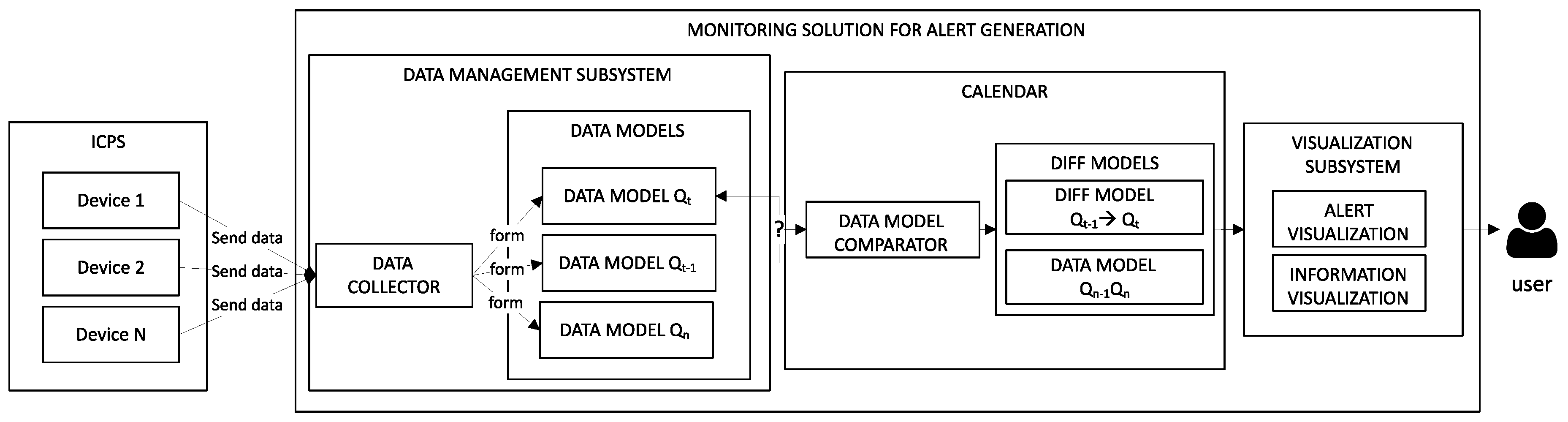
Figure 1 illustrates an overview of the monitoring of an ICPS and how an evolution can be detected by CALENDAR. CALENDAR is capable of detecting additions, removals, and modifications on an ICPS (e.g., integration of a new device) immediately (next time the data is received).
The monitoring system is composed of three subsystems: (1) the data management subsystem, responsible for capturing data from an ICPS and building the corresponding Data Models; (2) CALENDAR, responsible for analyzing the evolution occurred in the ICPS; and (3) the visualization subsystem, which is responsible for communicating to the user the evolution in a proper manner.
The data management subsystem uses Data Models to create a snapshot of the ICPS at a specific moment in time. Thanks to it, both the structure of the ICPS and the data are captured. Thus, from the received data, the Data Collector extracts a specific Data Model that saves all the information received from the ICPS at a given time as explained in our previous work [5].
Once the Data Model is formed by the Data Collector, CALENDAR starts working. It is important to know that CALENDAR is suitable once the evolution has occurred. CALENDAR is a reactive system, i.e., reacts to changes that have happened; it does not anticipate them.
Inside CALENDAR, the Data Model Comparator analyzes if any change has happened since the last time the data was received. In the case that any evolution occurred, CALENDAR is responsible for classifying the occurred evolution in a Diff Model.
ICPS evolves over time, so detecting changes in the structure such as the addition or removal of devices are critical to providing the user with the right information to make decisions. CALENDAR is responsible for detecting the evolution in an ICPS and its classification. For each Data Model, CALENDAR compares the current instance (Data Model Qt) with the previous instance in time (Data Model Qt-1) to identify the evolution of an ICPS. Diff Models are used to classify changes and to alert the user on the instat that evolution occurs through the visualization subsystem. In this way, the user is fully informed of what is happening and can, therefore, be supported in decision-making.
Thus, if the ICPS can be represented by the Data MetaModel, CALENDAR is able to analyze at runtime if any changes have occurred. Hence, CALENDAR is able to detect any evolution which can be represented by the Data MetaModel (presented in Section 4.1). For example, imagine that due to the intelligence of a device, this one starts sending a new attribute which was not previously represented in the Data Model. In this particular scenario, CALENDAR is able to detect a new attribute at runtime in addition to classifying it.
The visualization subsystem, already developed and evaluated in Reference [10], is capable of visualizing both the information (information visualization) and the alerts (alert visualization) to communicate changes to the user. Moreover, the subsystem is also responsible for managing the invalid visualizations, i.e., if the ICPS evolves (e.g., a device is removed), the visualization fails due to the fact that the information to be displayed has disappeared. Thus, the visualization subsystem is able to manage those situations so that the visualization is adequate in addition to informing users about the occurred changes.
CALENDAR ensures the detection of evolution in an ICPS. An ICPS faces changes frequently, and controlling them is necessary for users to make valid decisions. In the following sections, we detail CALENDAR and provide an evaluation that shows its applicability in real scenarios.
4. CALENDAR
In this section, we focus on CALENDAR, i.e., a system that compares the current instance (Data Model Qt) with the previous instance in time (Data Model Qt-1) to identify the evolution of an ICPS.
The objective of CALENDAR is to detect an ICPS evolution. Once an evolution occurrs, our solution is able to identify at any level, the additions, removals, or modifications by comparing Data Models in subsequent timestamps.
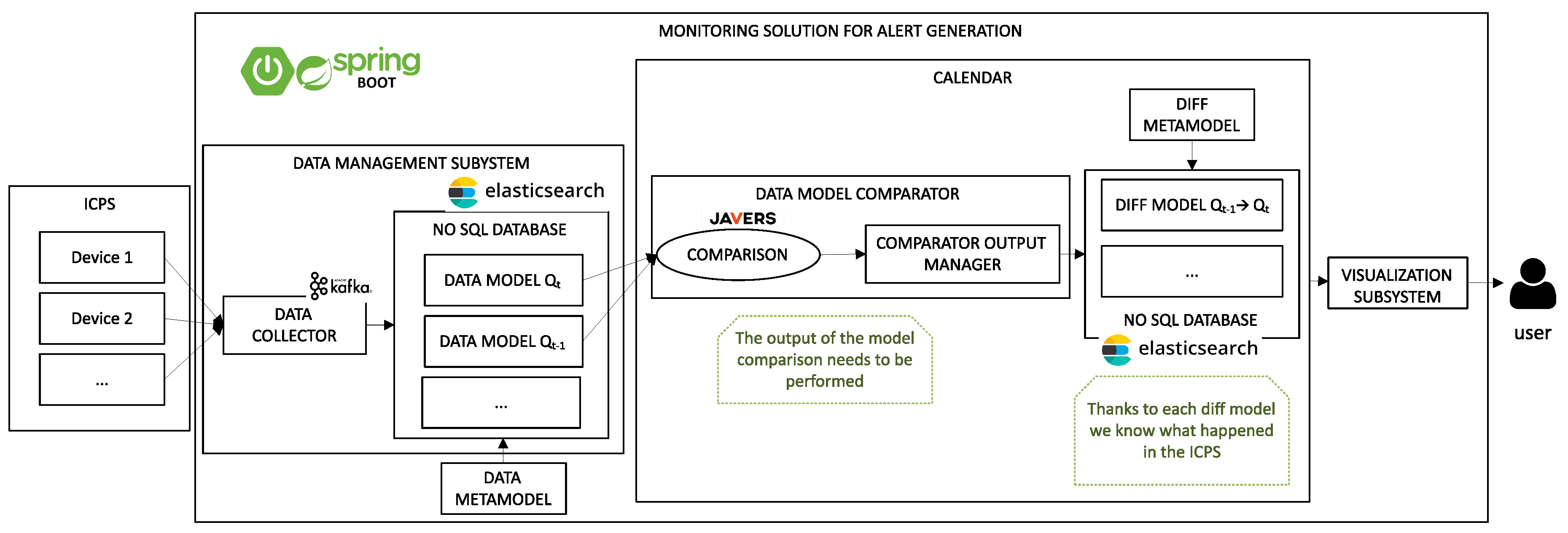
In Figure 2, the real scenario of monitoring an ICPS is presented, which was developed with SpringBoot. As mentioned above, the Data Collector, which is based on Kafka, is a distributed streaming platform that is responsible for generating the Data Models, taking into account the data received from the ICPS. Once the Data Model is created, it is stored by the Data Collector in a NoSQL database (Elasticsearch), so in this manner, CALENDAR can then use any stored Data Model.
Once the Data Model is stored and a new one is detected, CALENDAR starts working. CALENDAR is composed of two main components: (I) Data Model Comparator, the component responsible for comparing two subsequent Data Models, and (II) Diff Models, the instance of Diff MetaModel responsible classifying the occurred evolution.
In this section, first, we present the Data Models that CALENDAR is going to use in order to detect ICPS evolution (Section 4.1). We present the characteristics of the Data Model in order to define what kind of evolution will be able to detect. Then, in Section 4.2, how CALENDAR is able to compare two Data Models using the Data Model Comparator component is presented. Finally, in Section 4.3, the Diff Model where the result of the Data Model Comparator classification is explained.
4.1. Data MetaModel
The Data MetaModel is the artifact that allows a representation of both the data and structure at once. It has a tree structure to facilitate the evolution detection [24] and contains seven levels [5] that represent the logical and physical structures of different ICPSs. The Data MetaModel is a combination of two different standards (i.e., IEC 62264 and IEC 61850). In order to be valid this Data MetaModel in different ICPSs, the following requirements need to be considered:
- Quantity of levels: The Data Model conformed by the Data MetaModel will always be composed of 7 levels, i.e., there cannot be a branch containing only 5 of them.
- ICPS representation: The Data MetaModel has a hierarchical structure. This implies that a node of the Data Model cannot depend on several nodes, i.e., a single node contains a single parent node.
- Physical/logical structure: Even if in an ICPS, a node can communicate with other nodes, in our Data MetaModel, the relation between nodes is not reflected. Each node is independent of the rest. If we wanted to reflect the relation between nodes, another model must be used.
- Atomic values: Although the Data MetaModel supports complex data structures, we do not focus on the analysis of these complex data. That is why, the Data MetaModel is designed for atomic data values, i.e., simple data (e.g., Boolean, Integer, and String).
In addition, it is important to notice that these Data MetaModels are also valid for monitoring multiple ICPSs, i.e., multiple press lines. More information about the Data MetaModel is provided in Reference [5]. In the next table, information about each level of the Data MetaModel is provided:
Thus, the Data Collector generates a Data Model that conforms to this Data MetaModel in each timestamp. Once the Data Model is captured, the Data Model Comparator analyzes if any change has happened since the last time data was received.
4.2. Data Model Comparator
For each Data Model, the Data Model Comparator compares the current instance (Data Model Qt) with the previous instance in time (Data Model Qt-1) to identify the evolution of an ICPS. To perform the comparison between the two Data Models, CALENDAR uses Javers. Javers is a library able to compare complex structures and to detect changes. Javers’ output is not enough for our purpose so we have post-processed the results of Javers.
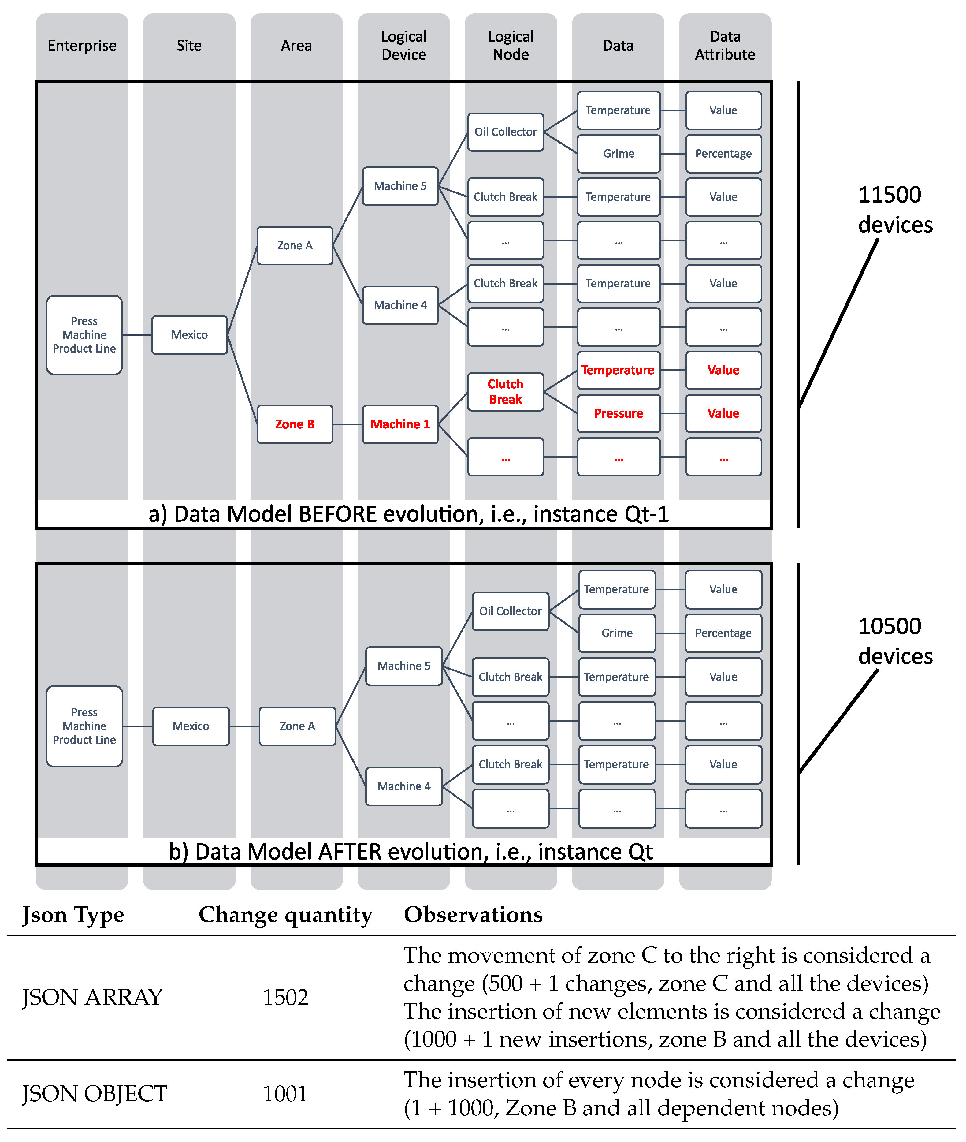
Notice that Javers does not take into account the hierarchical dependencies between nodes. However, the dependencies in an industrial environment are something necessary because it is valuable to visualize the result in a simple and meaningful way to the user in order to help him/her make decisions. That is why we need to post-process the Javers result. For example, in the press line domain due to business strategy, imagine it is necessary to remove Zone B. In the upper part of Figure 3, the Data Model before an evolution occurred (Qt-1) is shown, e.g., the Press Machine product line of Mexico is composed by two areas. However, in the lower part of the figure, the Data Model after an evolution (Qt) is presented, e.g., Zone B is removed from the Press Machine product line. Therefore, all nodes that depend on that zone are removed (e.g., Machine 1). When CALENDAR compares Qt with Qt-1 using Javers, this one detects a change for each modified, added, or removed node. In this case, Javers generates 1001 alerts when Zone B node is removed using a Json Object format or 1502 alerts using a Json Array format. This quantity of alerts do not facilitate the task to the user when data is represented. Even if the example given is due to a business strategy, note that, as mentioned in Section 3, many reasons can trigger the evolution of an ICPS, e.g., devices’ intelligence itself can cause changes in the Data Model. Additionally, it is important to notice that many people are supporting the monitoring system and that not all of them are interested in the same data or information [10]. In spite of that, all of them need to be informed about the occurred evolution.
Thus, we concluded that the comparison provided by Javers is format-dependent, i.e., the format of the text model impacts the result. If Json arrays [25] are used, the order is taken into account. Thus, when removing node Zone B, the nodes on the right are marked as modified, i.e., Zone C is marked as modified, ascending the number of alerts to 1502. Instead, if we use Json Objects [25], when the order of a node changes (due to an addition or removal), it is not marked as a change.
To overcome this limitation, besides using Json Objects, we post-process the Javers result and use a model to manage the post-procesed output, which only generates the necessary alerts for the user (Diff Model); in this particular case, we will only generate a unique alert, i.e., Zone B is removed.
4.3. Diff MetaModel
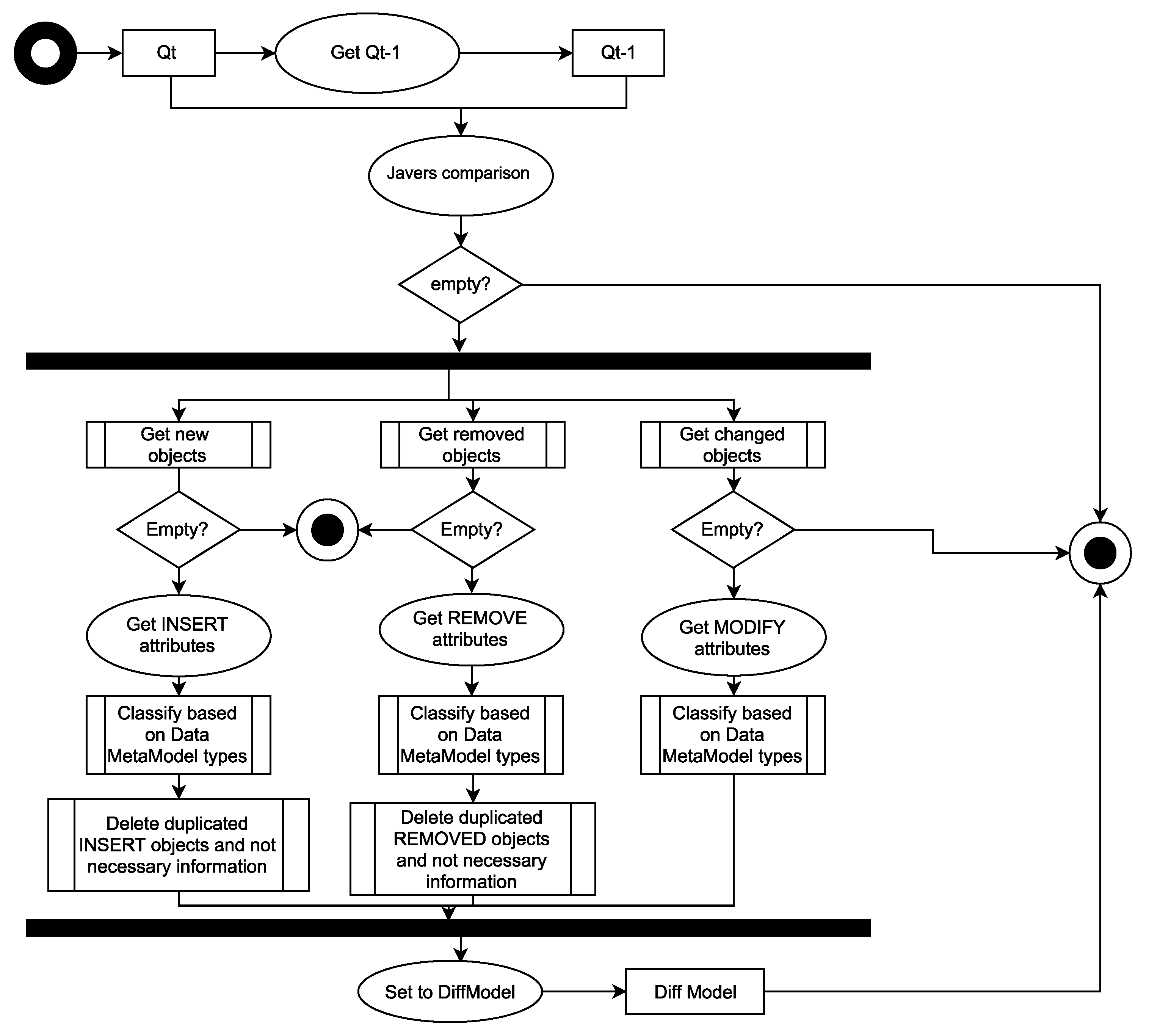
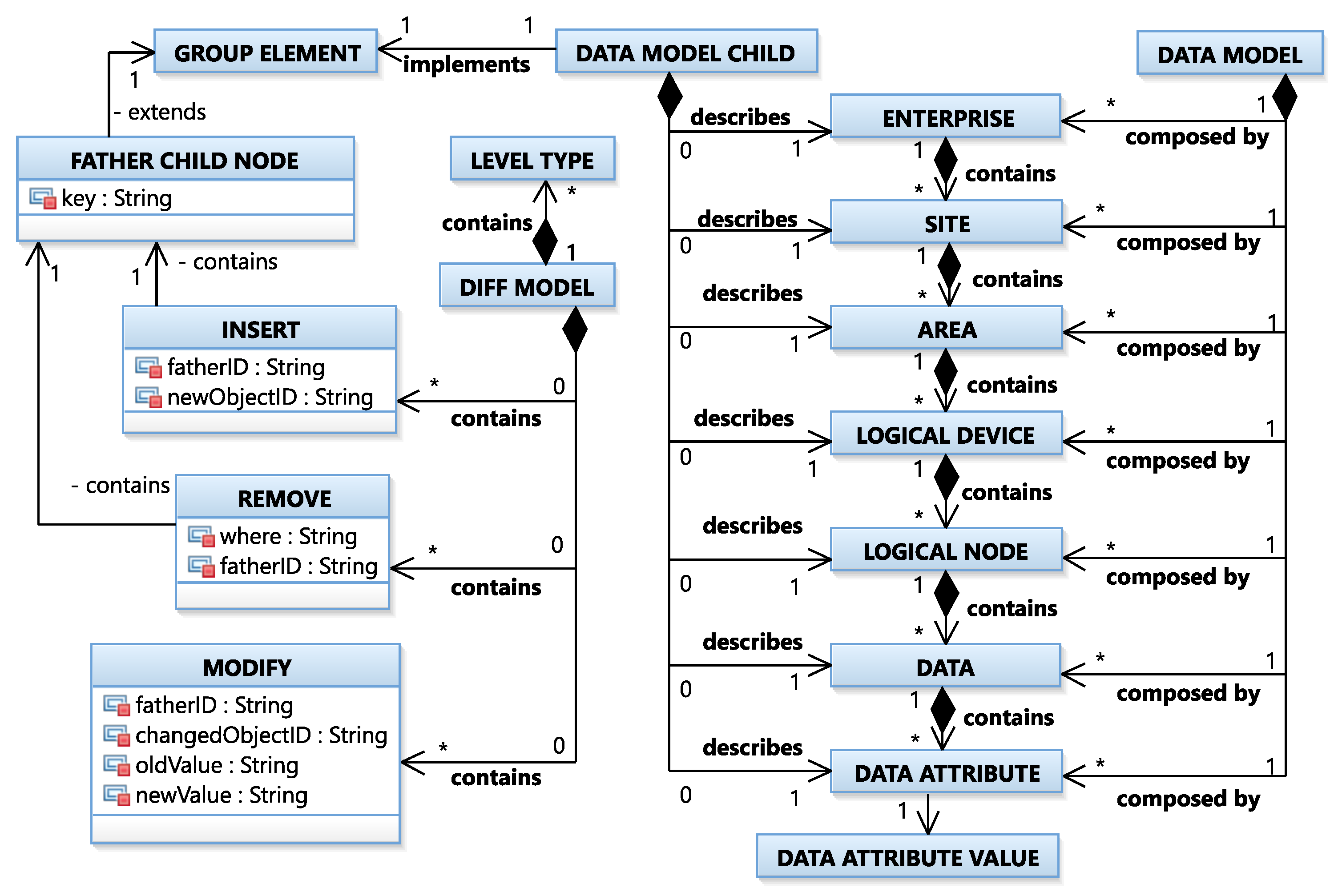
In Figure 4, a diagram of the process for creating the concrete Diff Model is presented. The process starts when a new Data Model is received, on the right side of Figure 5, the Unified Modeling Language (UML) diagram of the Data MetaModel is shown. In that moment, CALENDAR gets the received Data Model and the previous instance, i.e., Qt and Qt-1. Then, the Data Models are compared by the Data Model Comparator using Javers as explained in the previous section. If the result is not empty, CALENDAR gets the result of Javers and treats each action differently (new, remove, or change). This is because the information to be saved depends on the type of change that occurred. Once the attributes are mapped, the information is classified based on the Data MetaModel types (see Table 3). This manner simplifies to identify where the evolution has occurred. Then, if elements are added or removed, it is necessary to delete the unnecessary information despite duplicated information as mentioned above (e.g., from 1001 alerts to 1, i.e., we do not take into account nodes below Zone B). Finally, all the information is set to create the Diff Model. Once the process is finished, the created Diff Model is stored in a NoSQL database in order to keep track of the traceability of the occurred evolutions over time.
The Diff MetaModel contains information about the types of changes, the level in which the changes have occurred and the nodes affected by the changes. The level type is related to the level of the Data MetaModel and describes in which level of the Data Model the changes occurred (e.g., site). Therefore, the Diff Model can have a maximum of seven level types, one for each Data Model level. That is, all the identified changes in a level (e.g., area) are grouped. This classification facilitates communication among users.
Inside each level, the metamodel considers three types of changes that occur when an ICPS evolves (see Figure 5).
- ADD: all the new nodes that do not exist in the previous instant.
- REMOVE: all the nodes that have disappeared at the previous instant.
- MODIFY: if the node exists, but a change has happened in it.
To reduce the alerts of removal or addition explained in the previous section (i.e., "delete duplicated INSERTED/REMOVED objects and unneccesary information"; see functions of Figure 4), e.g., from 1001 alerts to 1 alert, a FatherChildNode is used to group the affected nodes, see Figure 5. The FatherChildNode is an instance of a DataModelChild, that is, a subtree with the node changed and its children and contains the nodes affected by an addition and removal. Note that the FatherChildNode does not need to contain the seven levels; despite this, the Data Model will always be composed of seven levels as mentioned in Section 4.1.
When a node is removed or inserted, a FatherChildNode is saved that extends from GroupElement i.e., the GroupElement describes the FatherChildNode, since it describes the DataModelChild. For example, Figure 3 only shows the first five levels (enterprise, site, area, logical device, and logical node); in a real scenario, it would be composed of seven levels. When Zone B is removed, the FatherChildNode would be composed of Zone B and its children, i.e., DataModelChild only contains five levels (area, logical device, logical node, data, and data attribute); the enterprise and site will not be saved. In this manner, we reduce the number of alerts. A description of each variable in the Diff MetaModel is presented in Table 4:
A Diff Model that conforms to a Diff MetaModel is created automatically from Javers output every timestamp, and then, it is stored in Elasticsearch. Thus, it is possible to classify all the changes so that they can be presented easily to the user. Thanks to this metamodel, the number of alerts are reduced and we avoid redundant information because we just save the deepest node that is changed, excluding all below nodes.
5. CALENDAR Evaluation: Scalability Test
Despite ICPS evolution, different ICPS Data Model sizes exist, e.g., a press machine can be composed of 50 or more than 1000 devices, this being one of the machines within the press line. In addition, a customer can also be interested in monitoring multiple press lines; thus, the size of the environment can be huge. In order to ensure the usability of CALENDAR in different ICPS sizes, we provide a scalability test.
The data to perform the scalability test were created in a random way, since we had no access to the real data to perform the scalability test. Thus, considering that the Data Collector generates every Data Model that conforms to the Data MetaModel, we simulate these Data Models randomly. In this way, we can also conclude that CALENDAR is applicable for other domains that use the Data MetaModel as a base, as long as the scenario to be monitored complies with the Data MetaModel characteristics presented in Section 4.1.
All the experiments have been performed on a laptop with a CPU Intel (R) Core (TM) i7-4600U CPI @ 2.10GHz CPU. In addition, the computer in use had a 16 GiB memory with a 64-bit operating system (Linux) and a 500-GB disk (HDD). The correctness of the Diff Models was tested manually with a smaller Data Model. Java Microbenchmark Harness (JMH) (https://www.baeldung.com/java-microbenchmark-harness) was used to execute an accurate microbenchmark in an automatic way, i.e., measure the average time that CALENDAR takes to run and the confidence interval of the average.
In order to get reliable numbers, each query was processed 200 times for each evaluation case and Java Virtual Machine was restarted for each execution for each test.
Considering that changes can occur in any of the Data Model levels but mostly that the evaluation occurs at the devices (i.e., Logical Node), in the evaluation, we simulate changes in this level. For the evaluation, as mentioned above, we randomly generated Data Models with 50, 100, 500, 1000, 5000, and 10,000 devices. Each Data Model was cloned and the changes were inserted: an addition, removal, modification, and random changes (addition, modification, and removal). Finally, we established different percentages of changes (from 20% to 100%). Note that 100% means an addition of 10,000 devices in the largest model or a modification of the devices. In the case of removal, we skipped the removal of 100%, as it would result in an invalid Data Model. The scalability test results are reflected in Appendix A and Table A1.
In this evaluation, we address “Which is the performance of CALENDAR?” To do so, we distinguish three different configuration factors (F) that may impact
- F1 → Type of change: We measure how the type of change (addition, modification, or removal) impacts the performance (execution time).
- F2 → Percentage of devices changed: We measure how the number of devices changed impacts the performance (execution time).
- F3 → Size of the Data Model: We measure how the increasing size of the Data Model impacts the performance (execution time).
5.1. Discussion
Considering all the results obtained, the following section discusses the factors F1, F2, and F3 as well as a joint analysis of them all. The results have been evaluated against the following quantitative metrics: AVG: Average Execution Time in milliseconds (ms) and CI: Confidence Interval (ms).
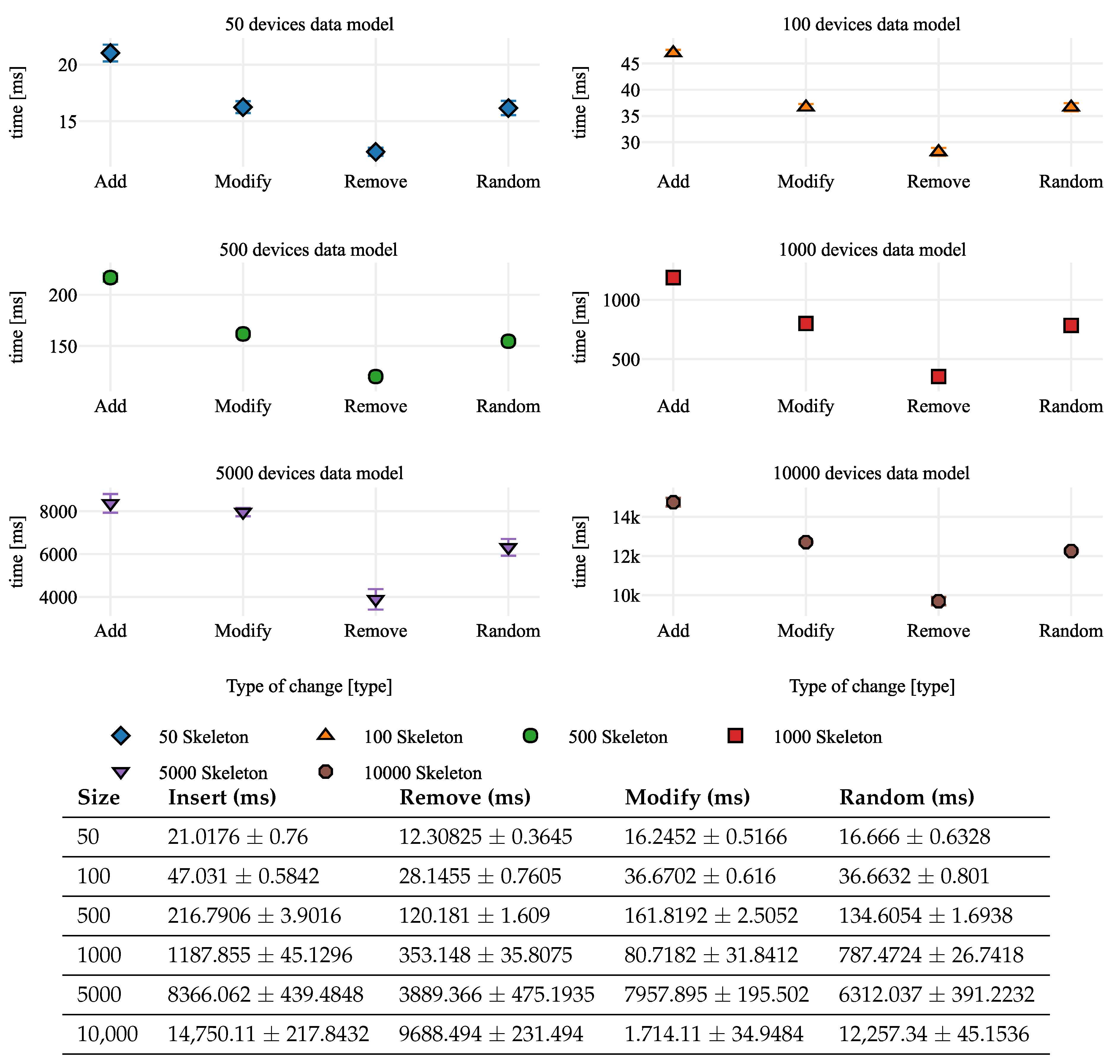
5.1.1. F1: Type of Change
In Figure 6, we show the different ICPS Data Models separated by the different changes, i.e., inserted, removed, or modified. The type of change seems to affect our system. That is, the detection of adding a device is not the same as detecting that a device is removed or modified. Taking, for example, the Data Model of 50 devices, the adding devices average is 21.0176 ms ± 0.738 ms, removing devices is 12.30825 ms ± 0.3645 ms, and modifying devices is 16.2452 ms ± 0.5166 ms. In the case where all kind of changes are made in the same Data Model (insert, remove, and modify), the time needed is 16.1666 ms ± 0.6328 ms. The difference between removing and inserting devices (maximum and minimum execution time) is about 71% for this Data Model.
Considering the differences between the highest and lowest execution times of all Data Models (see Table 5), we can conclude that it does not have a relation with the size of the Data Model. However, in all the cases, the difference between the maximum and the minimum is 50% up to 220%.
The type of change to detect and classify the evaluation affects the result. Thus, detecting removals is less expensive than detecting insertions in a Data Model. In the same way, the execution time for modifying devices is between adding and deleting. In the case of random changes, the maximum (insert) and minimum (remove) time are compensated, and therefore, the average time achieved is more or less in the middle.
5.1.2. F2: Percentage of Changes
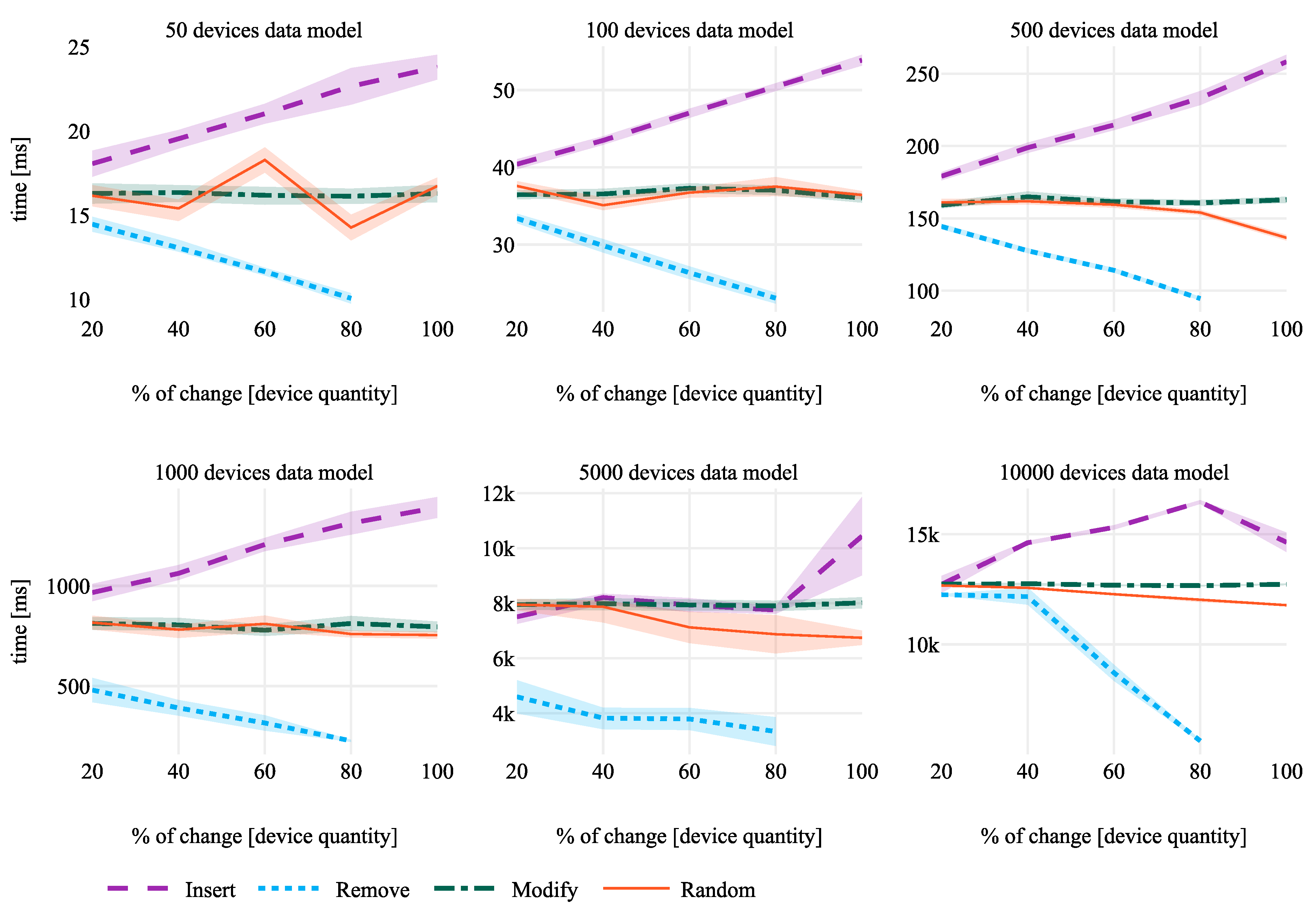
This factor evaluates whether the percentage change affects the execution time, i.e., if with the same Data Model (e.g., 1000 devices), changing 20% (e.g., 200) or 100% (e.g., 1000) of devices influences the time required (execution time) for detecting changes. The results are shown in Figure 7.
Considering the different changes that can occur, we observe that
- Inserting: The higher the percentage of change, the higher the execution time. In the smallest Data Model (50 devices), the execution time has an increase of 41.89%. With a bigger Data Model (e.g., 10000), the difference is 46.49%. Considering all the results (see Table 6), more or less of the difference between the minimum and maximum execution time when the percentage of change changes is between 40% and 60%. Therefore, as it is reflected in Figure 7, the growth of time is linear to the percentage of change.
- Removing: The lower the percentage of change made, the longer the execution time. In addition, the time decreases linearly. The execution time required for removing 20% in a 50 device Data Model is 14.462 ms, but in 80%, it is 10.06 ms. A difference of 52.86% exists, reaching 143.98% in the case of 1000 devices.
- Modifying: Increasing the percentage of change does not have a negative impact on time. The major percentage of change occurs with 1000 Data Model sizes, i.e., 0.013%. That is why we can concluded that the trend is constant.
- Random: This scenario is similar to modifying devices, i.e., increasing the percentage of change does not have a negative impact on the time, making the trend rather constant. Moroever, this is a case that depends a lot on the changes that have taken place.
Therefore, in a common scenario where we do not control over what is going on, we can assume that the percentage of change does not have a negative impact on the execution time needed. The times for adding and removing are compensated for each other, leaving a rather stable time when making random changes.
5.1.3. F3: Size of the Data Model
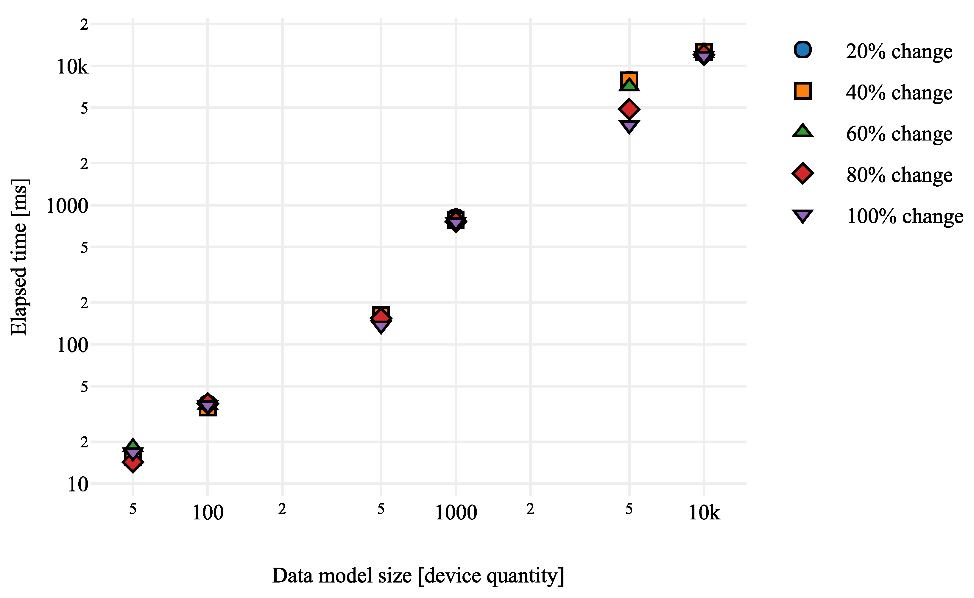
In order to see if the ICPS Data Model size affects the execution time needed, we extracted the values of the random test case (see Appendix A and Table A2). As we have concluded in factor F2, in a real scenario, we do not know about the change that is going to happen, and it has also been shown that time is more or less constant in terms of the number of changes that have occurred. In this manner, we contemplate all the cases without focusing on a single change. As it is shown in Figure 8, the larger the ICPS Data Model, the longer the execution time is. For detecting 100% of changes in a 1000 device Data Model, i.e., 1000 changes, CALENDAR needs an average of 754.174 ± 736.894 ms in contrast in the 5000 device Data Model detecting 20% of changes, i.e., for the same quantity of changes (1000), the time needed is bigger (7948.296 ± 7740.268 ms). For detecting the same quantity of changes, 546% more time is needed, i.e., equivalent to 6.6% of seconds. Looking at the graph, we know that this is not an isolated case; it is something that occurs if we compare different Data Model sizes. That means that the Data Model size, i.e., the input, impacts the output. The larger the size of the Data Model, the longer the time needed to calculate the differences even though the number of changes is the same.
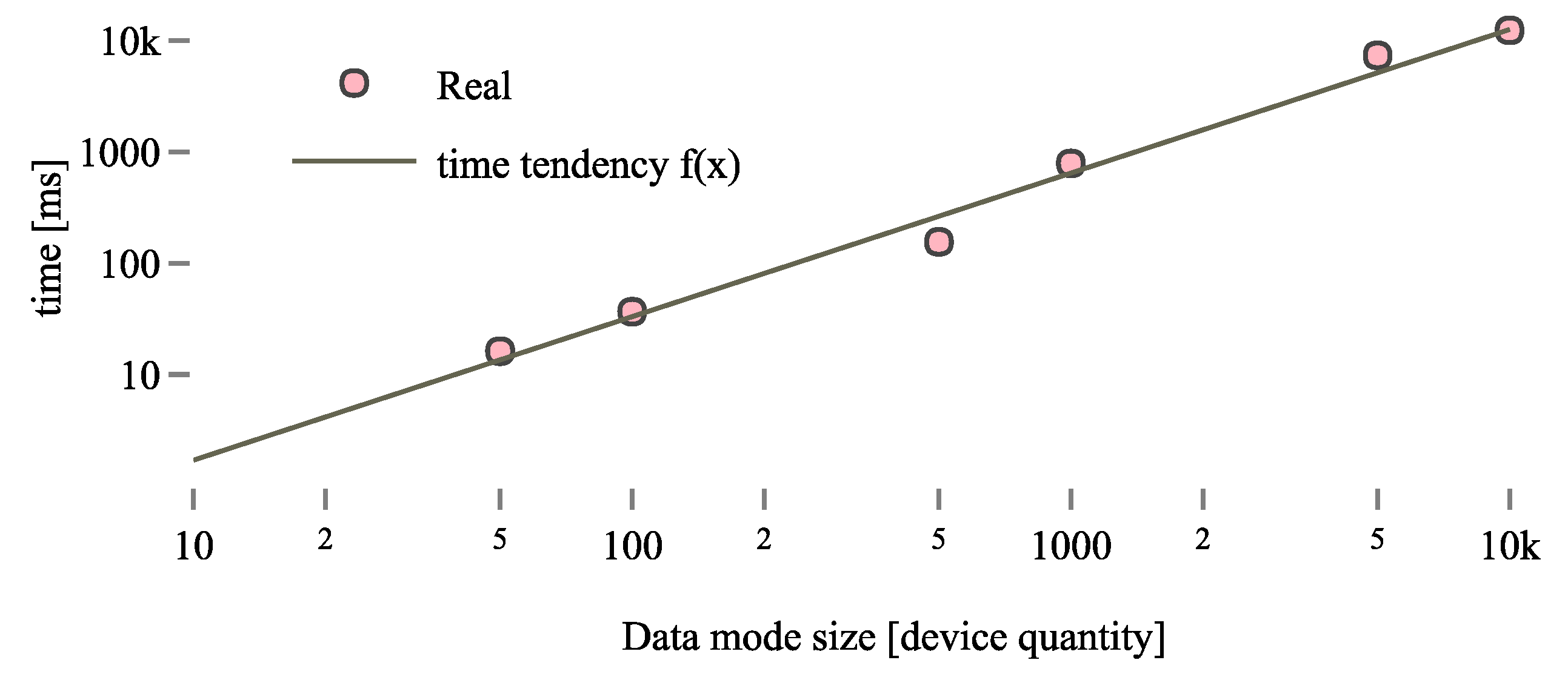
In order to see the trend that our system has, we calculated the average needed for each ICPS Data Model size (considering random changes results). Analyzing the results, we can observe that they tend in a potential way, which can be represented as follows: .
Thanks to a linear regression, i.e., a mathematical model used to approximate the relationship of dependence between a dependent variable (time) and the independent variables (quantity of devices), we obtain values and .
Thus, we obtain the equation , which is represented in Figure 9 and shows the relation between the ICPS Data Model size and the execution time.
Henceforth, using this solution with a high quantity of devices could be a problem, since if CALENDAR needs to be used in an ICPS with many devices, it is necessary to provide a solution to the scalability problem found in order to reduce the execution time. If a fast response is needed when the number of devices is high, this module would not be able to give a fast enough response to the user. For example, in a small (50 Data Model size) scenario, 0.016 ± 0.0006 s are needed, but in a bigger one (5000 Data Model size), 6.312 ± 0.3912 s are needed. Usually, the latency of an industrial monitoring system is about 2000 ms. That is why our system is not profitable enough in real-time big Data Model scenarios.
5.1.4. Factor Analysis (F1, F2, and F3)
Considering all factors, we realize that, with small Data Models, the average time that CALENDAR needs for communicating alerts is smaller. In the same manner, taking into account Figure 9, we see that the behavior of the small Data Models is smoother than that of the larger ones as the trends are clearer. Thus, currently, CALENDAR is able to give responses to small ICPSs as long as it meets the customer’s requirements, i.e., the latency is adequate.
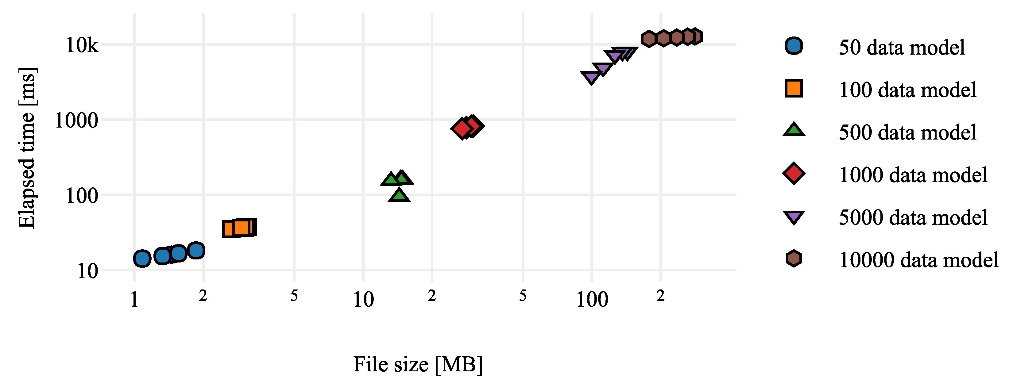
In industrial scenarios in which monitoring has a latency that does not support our solution, we propose to split the Data Model file into different files, making a comparison in each of the files. The following chart shows (Figure 10) the relation between the file size and the execution time, where it is shown that the smaller the file, the smaller the execution time.
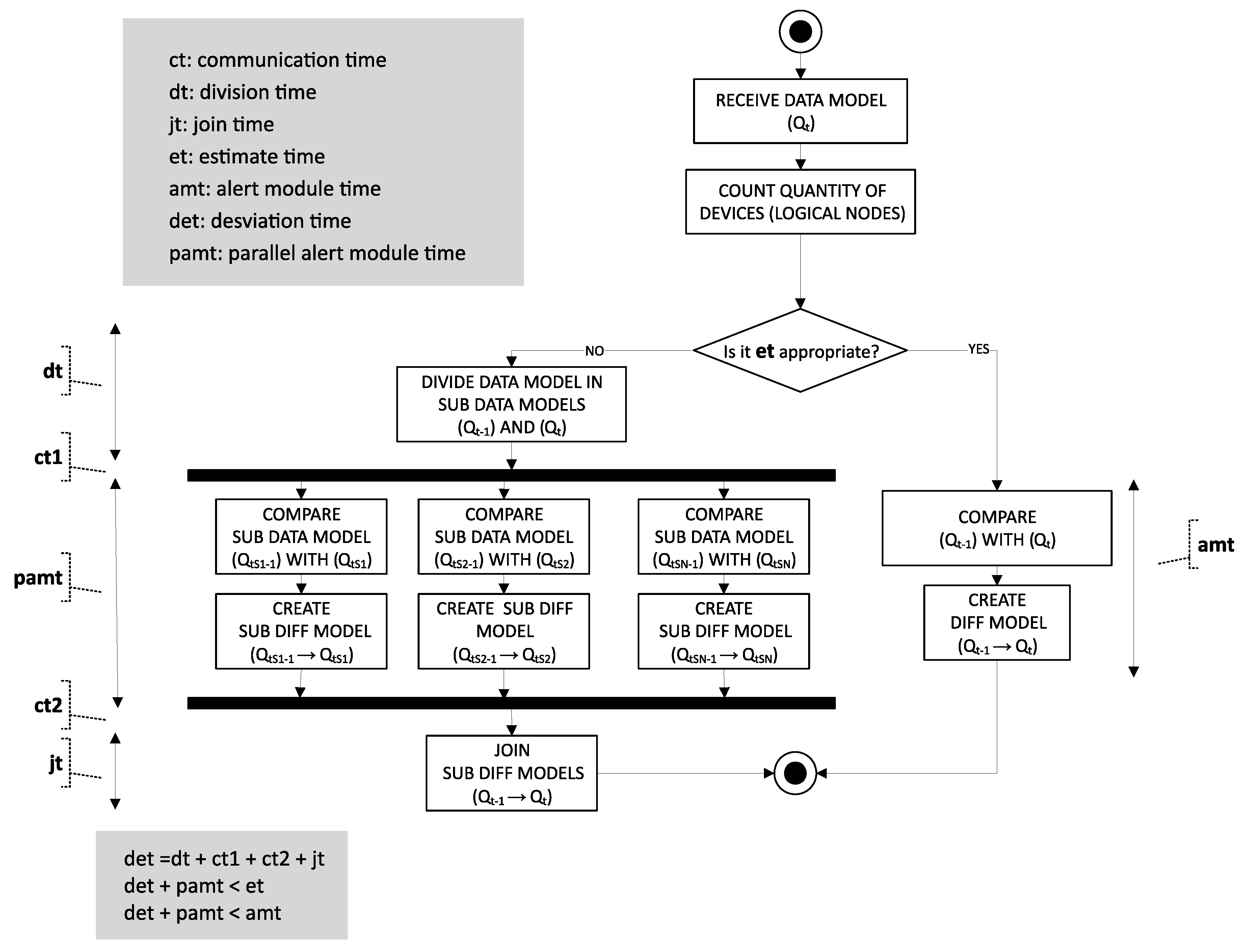
Taking into account the results of Figure 10, we propose a division of the Data Models into sub-Data Models. Because there are no data dependencies between the tasks to be parallelized, we can use the parallel computing theory to decrease the response time. Dividing the model, we get that each sub-Data Model is smaller and, thus, that the individual execution time needed will be smaller. In the same way, several sub-Data Models would be executed at the same time, so we would lower the total execution time. However, it is necessary to consider that a Deviation Time (det) exists, since time is needed to split the Data Model in sub-Data Models and then the result needs to be joined, i.e., the different sub-Diff Models need to be converted into a unique Diff Model to finally transfer the information to the user. In Figure 11 is shown an activity diagram where, using the parallel computing theory, we can reduce the execution time in order to give a response to the problem founded.
Note that, for dividing the Data Model into sub-Data Models, we need to calculate the optimal division value, i.e., the value that instructs in how many sub-Data Models we should separate the model. To do so, we need to consider: (I) the time tendency formula (Formula 2) and (II) the deviation time that the proposal will have (Figure 11). Thus, by developing this improvement and performing a scalability test, we will be able to calculate the deviation time. Once we have the deviation time, we will be prepared to calculate the corresponding function to obtain the optimal division value.
We make use of the parallel computing theory; dividing our Data Model in sub-Data Models and calculating the optimal division value, we will generate a model capable of dividing the Data Model in an efficient manner with the aim of parallelizing the comparison and, thus, reducing time. Furthermore, in Big Data scenarios, thanks to the Map & Reduce programming models, there would be no problem in parallelization. Thanks to the Map functions, the differences between the sub-Data Models will be founded, and then, the Reduce functions will join the results. Notice that this is only a hypothesis, which will need to be evaluated in the future.
5.2. Threats to Validity
As for internal validity, not all test cases are analyzed, i.e., we only evaluated the variability on the device level (Logical Node), and this may be a threat at the time of conclusion. Although, considering the personal interviews with our industrial partner, the most variable part has been evaluated (device variability), it would be interesting to examine other industrial domains to consider that it is applicable to them.
As for the external validity, an evaluation is not performed in a real environment, i.e., the computer used has fewer resources than a possible industrial PC. It is, therefore, appropriate to perform this test in a real environment in order to obtain more realistic results.
6. Related Work
There are some proposals in the literature that address monitoring solutions for ICPSs [19,21]. ICPS monitoring solutions are used in different domains such as traffic control and safety, manufacturing, or energy conservation [21,26]. In the same manner, some authors propose monitoring ICPSs to detect attacks that can affect the systems [27] or even for, storage data, data analysis, and the use of machine learning techniques to automatically update ICPS functionalities [28]. Despite that, different authors manage ICPS variability regarding the software [14,15], and a few of them consider hardware variability [18,19]. Hernandez and Reiff-Marganiec [18] propose a framework where smart objects start working in a autonomous way from a passive position to an active one. Unlike our system, these smart objects only consider variability at the Cyber Layer not in the Physical Layer. Chen et al. [19] recognizes variability at the Cyber and Physical Layers, but it is not able to manage the variability at runtime.
Therefore, ICPSs evolve throughout their lifetimes [11], but the previous presented solutions do not consider the traceability and the communication of the evolution at runtime. Note that managing the variability is crucial in Industry 4.0 [1,2,10], as the data captured from the ICPS are converted into information for decision-making. Note that the ICPS evolution includes not only software but also the addition, removal, and replacement of already installed devices [10,19], as ICPSs and their operating environment are highly dynamic due to, e.g., a deployment of autonomous devices. Therefore, flexibility and adaptation are the two required capabilities posing additional challenges for monitoring ICPSs [1,11,12].
Thus, even if the evolution of an ICPS is something known in the literature [13,14], as far as we know, no one in the literature has given a response to detecting ICPS evolution in order (1) to have the traceability of what has happened in an ICPS over time and (2) to communicate the evolution immediately to the users to avoid any bad decision. Additionally, note that the data structure changes when the ICPS evolves; that implies that new data need to be captured by the monitoring system in addition to being visualized as new information to the user. It is, therefore, necessary to manage the evolution, since different user roles exist and all must be informed.
Thus, in our solution, the data captured from the monitoring system is structured with tree models, since according to Reference [24], using a tree model structure facilitates the detection of an evolution. Tree models have been used in medicine (mutation tree) to identify the mutation of atoms, molecules, particle, etc. which are reflected in trees [29]. Melnik et al. use the comparison of models to then match the two trees in order to turn them into one [5]. Thus, tree-shaped models are recognized when it is necessary to detect evolution. Additionally, with a tree-shaped model, the structure beside the information is be transferred [30].
Thanks to tree models, the detection of an evolution is more immediate. This allows users to report what has happened at all times. For that, different methods for the comparison exist, which are used for tree-shaped models [24] such as SiDiff, UMLDiff, WinDiff, WinMerge, and SMDiff. Some are text comparators like SiDiff, and others are graphic comparators (UM-LDiff, WinDiff, WinMerge, and SMDiff). Although the graphics buyers show you the result visually, they are not suited for runtime use and our need is to find such changes at runtime. WinDiff (https://windiff.waxoo.com/) and WinMerge (http://winmerge.org/?lang=es) are line-based tools, i.e., changes will not be expressed at logic issues. Trip-wire (https://github.com/Tripwire/tripwire-open-source) is able to detect changes, but it is not able to detect which are the changes, and Remedy (http://www.bmcsoftware.es/it-solutions/remedy-itsm.html) is able to detect changes in the structure but not on the values. In our case, the whole architecture needs to be analyzed, i.e., the ICPS structure and the corresponding values. Cobana et al. and Weaver et al. have selected ad hoc solutions. The former one proposes an algorithm to compares XML files [31], and in our case, the information has a JSON format. In addition, the solution is for websites, and the movements inside the same father are considered changes, i.e., the format of the XML impacts the result; hence, it is not a valid solution for us. The latter instead [30], even if they are able to detect a change in a concrete moment in time, do not retain the traceability of changes. In addition, the output script must be saved and processed for it to be interpretable.
Inspired on these works, our proposal (CALENDAR) uses a tree-shaped model structure as input (i.e., the Data Model is the output of the monitoring system) for a comparison and detection of evolution. Each detected evolution is stored in a specific model (Diff model) in order to have the traceability of what has happened during the whole useful life of an ICPS. Among all the comparison methods available for tree-shaped mode, in our case, we have selected Javers, as in our previous work [10], it is shown that it is a model text comparator suitable for JSON format (tree-model structure) received from the ICPS.
The novelty of this paper lies in the following which, as far as we know, has not been addressed in the literature: (1) CALENDAR helps users to be informed immediately. (2) Thanks to CALENDAR, you can keep track of all changes that have happened over time, and thus, users can avoid any bad decisions. (3) With CALENDAR, we are able to classify the occurred evolution, reducing the quantity of alerts. (4) With the union of CALENDAR and the contribution published previously [10], the users will be able to receive graphical alerts.
7. Conclusions and Future Work
This paper presents CALENDAR, a Cyber-physicAL systEm evolutioN Detection and Alert geneRation System, in order to detect structural changes and to classify them in an efficient way when the ICPS evolves. Different changes (insertion, removal, or modification) can occur when an ICPS evolves; hence, it is necessary to alert the user in order to make correct decisions. For that, the ICPS is monitored and a data model is formed. The data model captures the structure and the information of the ICPS at every timestamp, and it has a tree structure. Then, in CALENDAR, a model text comparator is used to compare the data model received in a time (Qt), with the data model received in the previous time (Qt-1). The problem is that these comparators (e.g., Javers) do not take into account the dependencies between nodes. Due to this problem, the number of generated alerts grows, so Diff Models are used to classify these alerts, reducing the number of alerts and communicating the evolution to the user in a more direct way, avoiding redundant information.
Despite ICPSs evolution, different ICPS exist, i.e., a press line can be composed by different machines which are composed by different devices. For example, in a press line, a common machine is the press machine which can be composed of 50 or more than 1000 devices. Thus, considering that a press line is composed by different machines, the quantity of devices to monitor is high. In order to ensure the usability in different ICPSs, we provide an evaluation (scalability test) to evaluate different factors: (1) if the time needed to detect ICPS evolution is different depending on the occurred changes (insert, remove, or modify); (2) if the time needed to detect ICPS evolution is the same when varying the percentage of changes in the same tree structure; and (3) if the time needed to detect ICPS evolution is the same when the number of devices is different.
After performing the evaluation, we discuss the obtained results, considering the factors. We concluded that detecting a device addition is more costly than detecting eliminations, but they compensate each other when we analyze joint tests. The cost of detecting modifications is similar. In the same manner, when we analyze different percentage changes, we realize that, in a real scenario where different changes can occur even if the percentage of change changes, the execution time is mainly constant. Finally, when analyzing different data model sizes and when the number of devices increased, the execution time of CALENDAR increases.
Thus, we raise a problem, since the execution time increases sup-linearly as we increase the ICPS data model size. That is why, in the future, we would like to improve CALENDAR in order to reduce the response time, since our hypothesis says that, if we decrease the size of the input files and use parallel computing theory, we will be able to decrease the total execution time, enabling new real time scenarios.
Author Contributions
Conceptualization, A.I., G.S., and C.A.; data curation, A.I.; software, A.I., G.S., and C.A.; writing—original draft, A.I.; writing—review and editing, G.S. and C.A.
Funding
This work received funding from the Basque Government through the Elkartek program under the TEKINTZE project (Grant agreement No. KK-2018/00104).
Conflicts of Interest
The authors declare no conflict of interest. The funding sponsors had no role in the design of the study; in the collection, analyses, or interpretation of data; in the writing of the manuscript; or in the decision to publish the results.
Appendix A

Table A1.
The obtained results from the data model comparator. The average time (AVG) and confidence interval (CI) of the execution time needed (ms).
Table A1.
The obtained results from the data model comparator. The average time (AVG) and confidence interval (CI) of the execution time needed (ms).
| 50 Devices | ||||||||
| INSERT | MODIFY | REMOVE | RANDOM | |||||
| AVG | CI ± | AVG | CI ± | AVG | CI ± | AVG | CI ± | |
| 20 | 18.06 | 0.773 | 16.288 | 0.602 | 14.462 | 0.443 | 16.155 | 0.627 |
| 40 | 19.553 | 0.508 | 16.347 | 0.457 | 13.062 | 0.478 | 15.403 | 0.525 |
| 60 | 21.026 | 0.589 | 16.183 | 0.556 | 11.649 | 0.228 | 18.28 | 0.747 |
| 80 | 22.654 | 1.086 | 16.127 | 0.45 | 10.06 | 0.309 | 14.265 | 0.763 |
| 100 | 23.795 | 0.734 | 16.281 | 0.518 | - | - | 16.73 | 0.502 |
| 100 Devices | ||||||||
| INSERT | MODIFY | REMOVE | RANDOM | |||||
| AVG | CI ± | AVG | CI ± | AVG | CI ± | AVG | CI ± | |
| 20 | 40.398 | 0.645 | 36.449 | 0.561 | 33.38 | 0.611 | 37.586 | 0.618 |
| 40 | 43.483 | 0.529 | 36.547 | 0.674 | 29.791 | 0.91 | 35.09 | 1.005 |
| 60 | 47.029 | 0.555 | 37.289 | 0.629 | 26.35 | 0.823 | 36.723 | 0.639 |
| 80 | 50.377 | 0.492 | 37.03 | 0.611 | 23.061 | 0.698 | 37.501 | 1.235 |
| 100 | 53.868 | 0.7 | 36.036 | 0.605 | - | - | 36.416 | 0.508 |
| 500 Devices | ||||||||
| INSERT | MODIFY | REMOVE | RANDOM | |||||
| AVG | CI ± | AVG | CI ± | AVG | CI ± | AVG | CI ± | |
| 20 | 179.135 | 2.836 | 159.188 | 2.234 | 144.423 | 1.828 | 161.05 | 2.366 |
| 40 | 198.863 | 3.486 | 164.873 | 3.699 | 127.603 | 1.774 | 161.808 | 2.217 |
| 60 | 214.576 | 3.57 | 161.443 | 2.364 | 114.108 | 1.576 | 159.476 | 2.093 |
| 80 | 233.163 | 4.82 | 160.746 | 2.112 | 94.59 | 1.258 | 154.081 | 1.793 |
| 100 | 258.216 | 4.841 | 162.846 | 2.117 | - | - | 36.612 | 1.965 |
| 1000 Devices | ||||||||
| INSERT | MODIFY | REMOVE | RANDOM | |||||
| AVG | CI ± | AVG | CI ± | AVG | CI ± | AVG | CI ± | |
| 20 | 966.694 | 42.941 | 812.452 | 31.71 | 479.819 | 60.566 | 816.526 | 34.539 |
| 40 | 1062.361 | 41.325 | 805.063 | 34.992 | 390.658 | 39.605 | 781.418 | 23.924 |
| 60 | 1206.35 | 32.811 | 778.48 | 28.555 | 315.706 | 38.158 | 810.628 | 41.136 |
| 80 | 1312.73 | 56.793 | 812.255 | 37.455 | 226.409 | 4.901 | 759.616 | 16.87 |
| 100 | 1391.139 | 51.778 | 795.341 | 26.494 | - | - | 754.174 | 17.28 |
| 5000 Devices | ||||||||
| INSERT | MODIFY | REMOVE | RANDOM | |||||
| AVG | CI ± | AVG | CI ± | AVG | CI ± | AVG | CI ± | |
| 20 | 7504.666 | 253.046 | 7948.106 | 192.028 | 4599.335 | 601.986 | 7948.296 | 208.028 |
| 40 | 8207.304 | 137.2 | 7983.115 | 199.595 | 3825.186 | 376.088 | 7871.655 | 223.714 |
| 60 | 7932.337 | 251.416 | 7937.625 | 195.618 | 3794.048 | 401.019 | 7123.38 | 570.081 |
| 80 | 7751.169 | 133.73 | 7906.775 | 186.239 | 3338.893 | 521.681 | 4872.885 | 694.389 |
| 100 | 10,434.83 | 1422.032 | 8013.856 | 204.03 | - | - | 3743.969 | 259.904 |
| 10,000 Devices | ||||||||
| INSERT | MODIFY | REMOVE | RANDOM | |||||
| AVG | CI ± | AVG | CI ± | AVG | CI ± | AVG | CI ± | |
| 20 | 12,723.95 | 383.693 | 12,734.7 | 42.86 | 12,254.94 | 33.845 | 12,671.83 | 43.162 |
| 40 | 14,616.28 | 82.877 | 12,754.4 | 35.86 | 12,168.72 | 402.94 | 12,565.88 | 52.22 |
| 60 | 15,310.77 | 97.376 | 12,685.11 | 28.597 | 8709.968 | 363.877 | 12,277.84 | 34.849 |
| 80 | 16,461.61 | 85.731 | 12,666.93 | 28.371 | 5620.353 | 52.583 | 11,991.42 | 67.946 |
| 100 | 14,637.95 | 439.539 | 12,729.39 | 39.054 | - | - | 11,779.71 | 27.591 |
Table A2.
The Data Model sizes in MegaBytes (MBs) for comparison.
| Size | Qt-1 (MB) | Qt (kb) | |||||
|---|---|---|---|---|---|---|---|
| Change | 20% | 40% | 60% | 80% | 100% | ||
| 50 | 1.515 | Remove | 1.212 | 911 | 609 | 307 | – |
| Insert | 1.811 | 2.105 | 2.399 | 2.698 | 2.993 | ||
| Modify | 1.513 | 1.506 | 1.500 | 1.496 | 1.494 | ||
| Random | 1.453 | 1.328 | 1.862 | 1.082 | 1.558 | ||
| 100 | 3.024 | Remove | 2.420 | 1.818 | 1.212 | 609 | – |
| Insert | 3.614 | 4.208 | 4.795 | 5.391 | 5.979 | ||
| Modify | 3.017 | 3.007 | 3.000 | 2.990 | 3.026 | ||
| Random | 3.136 | 2.655 | 3.035 | 3.057 | 2.930 | ||
| 500 | 15.106 | Remove | 12.083 | 9.066 | 6.043 | 3.024 | – |
| Insert | 18.057 | 21.018 | 23.980 | 26.924 | 29.877 | ||
| Modify | 15.065 | 15.022 | 14.974 | 14.928 | 14.888 | ||
| Random | 14.891 | 14.592 | 14.692 | 13.246 | 14.385 | ||
| 1000 | 30.212 | Remove | 24.161 | 18.127 | 12.086 | 6.045 | – |
| Insert | 36.119 | 42.028 | 47.941 | 53.837 | 59.751 | ||
| Modify | 30.115 | 30.036 | 29.944 | 29.846 | 29.770 | ||
| Random | 30.266 | 28.287 | 29.701 | 27.107 | 27.071 | ||
| 5000 | 147 | Remove | 117 | 88.4 | 59 | 29.5 | – |
| Insert | 176 | 205 | 234 | 263 | 292 | ||
| Modify | 147 | 146 | 146 | 145 | 145 | ||
| Random | 143 | 136 | 126 | 112 | 99.6 | ||
| 10000 | 294 | Remove | 235 | 176 | 118 | 58.9 | – |
| Insert | 294 | 411 | 469 | 295 | 585 | ||
| Modify | 294 | 293 | 192 | 291 | 290 | ||
| Random | 282 | 262 | 235 | 206 | 178 | ||
References
- Leitão, P.; Colombo, A.W.; Karnouskos, S. Industrial automation based on cyber-physical systems technologies: Prototype implementations and challenges. Comput. Ind. 2016, 81, 11–25. [Google Scholar] [Green Version]
- Lee, J.; Bagheri, B.; Kao, H.A. A Cyber-Physical Systems architecture for Industry 4.0-based manufacturing systems. Manuf. Lett. 2015, 3, 18–23. [Google Scholar] [CrossRef]
- Ruppert, T.; Jaskó, S.; Holczinger, T.; Abonyi, J. Enabling Technologies for Operator 4.0: A Survey. Appl. Sci. 2018, 8, 1650. [Google Scholar] [CrossRef]
- Rajkumar, R.; Lee, I.; Sha, L.; Stankovic, J. Cyber-physical systems: The next computing revolution. In Proceedings of the 47th Design Automation Conference, Anaheim, CA, USA, 13–18 June 2010; pp. 731–736. [Google Scholar]
- Iglesias, A.; Lu, H.; Arellano, C.; Yue, T.; Ali, S.; Sagardui, G. Product Line Engineering of Monitoring Functionality in Industrial Cyber-Physical Systems: A Domain Analysis. In Proceedings of the 21 st International Systems and Software Product Line Conference, Sevilla, Spain, 25–29 September 2017; pp. 195–204. [Google Scholar]
- Lee, J.; Kao, H.A.; Yang, S. Service Innovation and Smart Analytics for Industry 4.0 and Big Data Environment. Procedia Cirp 2014, 16, 3–8. [Google Scholar] [CrossRef] [Green Version]
- Bagozi, A.; Bianchini, D.; Antonellis, V.D.; Marini, A.; Ragazzi, D. Big Data Summarisation and Relevance Evaluation for Anomaly Detection in Cyber Physical Systems. In Proceedings of the On the Move to Meaningful Internet Systems. OTM 2017 Conferences—Confederated International Conferences: CoopIS, C&TC, and ODBASE 2017, Rhodes, Greece, 23–27 October 2017; Springer International Publishing: New York, NY, USA, 2017; pp. 429–447. [Google Scholar]
- Stojanovic, L.; Dinic, M.; Stojanovic, N.; Stojadinovic, A. Big-data-driven anomaly detection in industry (4.0): An approach and a case study. In Proceedings of the 2016 IEEE International Conference on Big Data, BigData 2016, Washington, DC, USA, 5–8 December 2016; pp. 1647–1652. [Google Scholar]
- De, S.; Zhou, Y.; Larizgoitia Abad, I.; Moessner, K. Cyber–Physical–Social Frameworks for Urban Big Data Systems: A Survey; Multidisciplinary Digital Publishing Institute: Basel, Switzerland, 2017; Volume 7, p. 1017. [Google Scholar]
- Iglesias, A.; Arellano, C.; Yue, T.; Ali, S.; Sagardui, G. Model- Based Personalized Visualization System for Monitoring Evolving Industrial Cyber-Physical System. In Proceedings of the 25th Asia-Pacific Software Engineering Conference, APSEC 2018, Nara, Japon, 4–7 December 2018. [Google Scholar]
- García-Valls, M.; Perez-Palacin, D.; Mirandola, R. Time-Sensitive Adaptation in CPS through Run-Time Configuration Generation and Verification. In Proceedings of the IEEE 38th Annual Computer Software and Applications Conference, COMPSAC 2014, Vasteras, Sweden, 21–25 July 2014; pp. 332–337. [Google Scholar]
- Gerostathopoulos, I.; Bures, T.; Hnetynka, P.; Keznikl, J.; Kit, M.; Plasil, F.; Plouzeau, N. Self-adaptation in software-intensive cyber-physical systems: From system goals to architecture configurations. J. Syst. Softw. 2016, 122, 378–397. [Google Scholar] [CrossRef]
- Schütz, D.; Wannagat, A.; Legat, C.; Vogel-Heuser, B. Development of PLC-Based Software for Increasing the Dependability of Production Automation Systems. IEEE Trans. Ind. Inform. 2013, 9, 2397–2406. [Google Scholar] [CrossRef]
- Bougouffa, S.; Meßzmer, K.; Cha, S.; Trunzer, E.; Vogel-Heuser, B. Industry 4.0 interface for dynamic reconfiguration of an open lab size automated production system to allow remote community experiments. In Proceedings of the 2017 IEEE International Conference on Industrial Engineering and Engineering Management (IEEM), Singapore, 10–13 December 2017; pp. 2058–2062. [Google Scholar]
- Tang, H.; Li, D.; Wang, S.; Dong, Z. CASOA: An Architecture for Agent-Based Manufacturing System in the Context of Industry 4.0. IEEE Access 2018, 6, 12746–12754. [Google Scholar] [CrossRef]
- Aicher, T.; Spindler, M.; Fottner, J.; Vogel-Heuser, B. Analyzing the industrial scalability of backwards compatible intralogistics systems. Prod. Eng. 2018, 12, 297–307. [Google Scholar] [CrossRef] [Green Version]
- Mauro, J.; Nieke, M.; Seidl, C.; Yu, I.C. Context-aware reconfiguration in evolving software product lines. Sci. Comput. Program. 2018, 163, 139–159. [Google Scholar] [CrossRef]
- Hernandez, M.E.P.; Reiff-Marganiec, S. Towards a Software Framework for the Autonomous Internet of Things. In Proceedings of the 4th IEEE International Conference on Future Internet of Things and Cloud, FiCloud 2016, Vienna, Austria, 22–24 August 2016; pp. 220–227. [Google Scholar]
- Chen, Z.; Zhang, X.; He, K. Research on the Technical Architecture for Building CPS and Its Application on a Mobile Phone Factory. In Proceedings of the 5th International Conference on Enterprise Systems, Beijing, China, 22–24 September 2017; pp. 76–84. [Google Scholar]
- Lei, Y.; Li, N.; Guo, L.; Li, N.; Yan, T.; Lin, J. Machinery health prognostics: A systematic review from data acquisition to RUL prediction. Mech. Syst. Signal Process. 2018, 104, 799–834. [Google Scholar] [CrossRef]
- Iglesias, A.; Iglesias-Urkia, M.; López-Davalillo, B.; Charramendieta, S.; Urbieta, A. TRILATERAL: Software Product Line based multidomain IoT artifact generation for Industrial CPS. In Proceedings of the 7th International Conference on Model-Driven Engineering and Software Development, Modelsward 2019, Prague, Czech Republic, 20–22 February 2019. [Google Scholar]
- Huang, L.; Gromiha, M.M.; Ho, S. iPTREE-STAB: Interpretable decision tree based method for predicting protein stability changes upon mutations. Bioinformatics 2007, 23, 1292–1293. [Google Scholar] [CrossRef] [PubMed]
- Lee, J.H.; Ahn, C.W. An Evolutionary Approach to Driving Tendency Recognition for Advanced Driver Assistance Systems. In Proceedings of the MATEC Web of Conferences, EDP Sciences: 8th International Conference on Computer and Automation Engineering (ICCAE 2016), Melbourne, Australia, 3–4 March 2016; Volume 56, p. 02012. [Google Scholar]
- Sebastiani, M.; Supiratana, P. Tracing the Differences on an Evolving Software Model. In Proceedings of the IRCSE ’08: IDT Workshop on Interesting Results in Computer Science and Engineering; Mälardalen University: Västerås, Sweden, 2008. [Google Scholar]
- Bo, Y. Querying JSON Streams. Ph.D. Thesis, Uppsala University, Uppsala, Sweden, 2010. [Google Scholar]
- Lee, E.A. Cyber Physical Systems: Design Challenges. In Proceedings of the 11th IEEE International Symposium on Object-Oriented Real-Time Distributed Computing (ISORC), Orlando, FL, USA, 5–7 May 2008; pp. 363–369. [Google Scholar]
- Pasqualetti, F.; Dörfler, F.; Bullo, F. Attack Detection and Identification in Cyber-Physical Systems. IEEE Trans. Autom. Control 2013, 58, 2715–2729. [Google Scholar] [CrossRef] [Green Version]
- Niggemann, O.; Biswas, G.; Kinnebrew, J.S.; Khorasgani, H.; Volgmann, S.; Bunte, A. Data-Driven Monitoring of Cyber-Physical Systems Leveraging on Big Data and the Internet-of-Things for Diagnosis and Control. In Proceedings of the 26th International Workshop on Principles of Diagnosis (DX-2015) Co-Located with 9th IFAC Symposium on Fault Detection, Supervision and Safety for Technical Processes (Safeprocess 2015), Paris, France, 31 August–3 September 2015; pp. 185–192. [Google Scholar]
- Chao, H.; Li, H.; Wang, T.; Li, X.; Liu, B. An accurate algorithm for computing mutation coverage in model checking. In Proceedings of the 2016 IEEE International Test Conference, ITC 2016, Fort Worth, TX, USA, 15–17 November 2016; pp. 1–10. [Google Scholar]
- Weaver, G.A.; Smith, S.W.; Bobba, R.B.; Rogers, E.J. Re-engineering Grep and Diff for NERC CIP. In Proceedings of the 2012 IEEE Power and Energy Conference at Illinois, Champaign, IL, USA, 24–25 February 2012; pp. 1–8. [Google Scholar]
- Cobena, G.; Abiteboul, S.; Marian, A. Detecting Changes in XML Documents. In Proceedings of the 18th International Conference on Data Engineering, San Jose, CA, USA, 26 February–1 March 2002; pp. 41–52. [Google Scholar]
Figure 1.
An overview of monitoring Industrial Cyber-Physical Systems (ICPSs): the captured data and detected evolution to alert users.
Figure 1.
An overview of monitoring Industrial Cyber-Physical Systems (ICPSs): the captured data and detected evolution to alert users.

Figure 2.
A real scenario of monitoring ICPS, detecting the evolution, and alerting users.

Figure 3.
Text model comparator operations depending on the input.

Figure 4.
The Diff Model creation a diagram.

Figure 5.
The Diff MetaModel structure for alerting users about ICPS evolution.

Figure 6.
The execution time averages in different ICPS Data Model sizes.

Figure 7.
The increase in the percentage of changes in different ICPS Data Model sizes.

Figure 8.
The time need for detection versus ICPS Data Model sizes (the axes are in logarithmic scale).
Figure 8.
The time need for detection versus ICPS Data Model sizes (the axes are in logarithmic scale).

Figure 9.
The time growth trend when we increase the number of devices (the axes are in logarithmic scale).
Figure 9.
The time growth trend when we increase the number of devices (the axes are in logarithmic scale).

Figure 10.
The relation between different Data Model file sizes and the elapsed execution time (the axes are in logarithmic scale).
Figure 10.
The relation between different Data Model file sizes and the elapsed execution time (the axes are in logarithmic scale).

Figure 11.
An activity diagram for reducing the alert module result time.

Table 1.
The characteristics of a Press Machine.
| Press Machine Characteristics | Product Scale | ||
|---|---|---|---|
| Small | Medium | Large | |
| Average number of devices per Press Machine | 20 to 49 | 50 to 99 | >500 |
| Percentage of affected devices when the Press Machine evolves (added, removed, or modified)? | 40% to 59% | 40% to 59% | 40% to 59% |
Table 2.
The user roles for press line supervision.
| Role | Definition |
|---|---|
| Operator | Controls the operation of the press line. |
| Analytical Manager | Analyzes the historical data in order to to find machine patterns or trends. |
| Domain expert | Analyzes at runtime the raw data of a specific device or group of devices to detect any malfunction or anomaly. |
| Technical Assistant | Provides technical assistance, i.e., people in charge to solve any incidence that can occurred as fast as possible |
| Assistance management | If an incident cannot be solved by the Technical Assistants, a more exhaustive assistance has to be planned. Thus, in that case, the issue will be transferred to the Assistance Management in order to solve the incidence. |
Table 3.
The level types of the Data MetaModel.
| Level Type | Descriptions |
|---|---|
| Enterprise | ICPS identification, name |
| Site | Geographical or physical distribution of the ICPS |
| Area | Logical distribution inside the ICPS |
| Logical device | Devices description |
| Logical node | Device identification |
| Data | Information description that the devices send |
| Data attribute | Concrete information that the device sends inside the data. |
Table 4.
A description of the information saved in each Diff Model.
| Variable | Description |
|---|---|
| father_ID | The identifier of the node from which an element has been added, deleted, or changed. |
| newObjectID | The identification of the newly inserted node |
| where | A path pointing to the entire chain from the enterprise to the newly inserted object. |
| FatherChildNode | The tree that depends on the inserted or deleted node. This tree does not necessary have seven levels; it will depend on the fatherID level. |
| changedObjectID | The identification of the changed node |
| oldValue | The value previously held by that node |
| newValue | The value currently held by the node |
Table 5.
The max and min execution time difference percentages.
| 50 | 100 | 500 | 1000 | 5000 | 10000 | |
|---|---|---|---|---|---|---|
| The difference between insert and remove | 71% | 67% | 80% | 224% | 115% | 52% |
Table 6.
The difference between the minimum (remove) and maximum (insert) execution times.
| 50 | 100 | 500 | 1000 | 5000 | 10000 | |
|---|---|---|---|---|---|---|
| % of ADD | 41.89 | 37.27 | 49.21 | 56.20 | 63.51 | 46.49 |
| % of MODIFY | 7.19 | 7.02 | 7.40 | 12.57 | 6.44 | 0.60 |
| % of REMOVE | 52.86 | 52.00 | 56.70 | 143.96 | 84.63 | 120.71 |
| % of RANDOM | 40.92 | 12.08 | 7.71 | 15.49 | 134.10 | 8.19 |
© 2019 by the authors. Licensee MDPI, Basel, Switzerland. This article is an open access article distributed under the terms and conditions of the Creative Commons Attribution (CC BY) license (http://creativecommons.org/licenses/by/4.0/).
Share and Cite
MDPI and ACS Style
Iglesias, A.; Sagardui, G.; Arellano, C. Industrial Cyber-Physical System Evolution Detection and Alert Generation. Appl. Sci. 2019, 9, 1586. https://0-doi-org.brum.beds.ac.uk/10.3390/app9081586
AMA Style
Iglesias A, Sagardui G, Arellano C. Industrial Cyber-Physical System Evolution Detection and Alert Generation. Applied Sciences. 2019; 9(8):1586. https://0-doi-org.brum.beds.ac.uk/10.3390/app9081586
Chicago/Turabian StyleIglesias, Aitziber, Goiuria Sagardui, and Cristobal Arellano. 2019. "Industrial Cyber-Physical System Evolution Detection and Alert Generation" Applied Sciences 9, no. 8: 1586. https://0-doi-org.brum.beds.ac.uk/10.3390/app9081586
Note that from the first issue of 2016, this journal uses article numbers instead of page numbers. See further details here.