Article

Compound Faults Feature Extraction for Rolling Bearings Based on Parallel Dual-Q-Factors and the Improved Maximum Correlated Kurtosis Deconvolution

1
Key Laboratory of Advanced Manufacturing Technology, Beijing University of Technology, Chao Yang District Beijing 100124, China
2
School of Mechanical and Electrical Engineering, Beijing University of Chemical Technology, Beijing 100029, China
*
Author to whom correspondence should be addressed.
Submission received: 12 March 2019 / Revised: 17 April 2019 / Accepted: 19 April 2019 / Published: 23 April 2019
(This article belongs to the Special Issue Fault Diagnosis of Rotating Machine)

Abstract

:
Vibration analysis is one of the main effective ways for rolling bearing fault diagnosis, and a challenge is how to accurately separate the inner and outer race fault features from noisy compound faults signals. Therefore, a novel compound fault separation algorithm based on parallel dual-Q-factors and improved maximum correlation kurtosis deconvolution (IMCKD) is proposed. First, the compound fault signal is sparse-decomposed by the parallel dual-Q-factor, and the low-resonance components of the signal (compound fault impact component and small amount of noise) are obtained, but it can only highlight the impact of compound faults, and failed to separate the inner and outer race compound fault signal. Then, the MCKD is improved (IMCKD) by optimizing the selection of parameters (the shift order M and the filter length L) based on the iterative calculation method with the Teager envelope spectral kurtosis (TEK) index. Finally, after the composite fault signal is filtered and de-noised by the proposed method, the inner and outer race fault signals are obtained respectively. The fault characteristic frequency is consistent with the theoretical calculation value. The results show that the proposed method can efficiently separate the mixed fault information and avoid the mutual interference between the components of the compound fault.

1. Introduction

Rolling bearing is one of the most widely used parts in rotating machinery. The operational status of the rolling element bearing often directly affects the performance of the whole machine. Consequently, the fault identification and diagnosis of rolling bearings are of great significance to ensure the safe and reliable operation of mechanical equipment [1,2,3]. Vibration signals caused by rolling bearing faults have been extensively studied and powerful diagnostic methods have been proposed. In recent years, the emerging artificial intelligence diagnosis technologies have been widely concerned by many scholars. A large number of artificial intelligent methods such as support vector machine [4], fuzzy diagnosis method [5], convolutional neutral network [6], and recurrent neutral network [7] were proposed to diagnose the mechanical faults. Furthermore, the sparse representation methods have also been widely used because of the signals sparsity. Adaptive impulse dictionary [8], combined time-frequency dictionary [9], matching pursuit [10], and dictionary learning method [11] were presented to diagnose faults of rotating machinery. In addition to the above mentioned two popular methods, many other research methods such as fault quantitative diagnosis [12], fault mechanism research [13,14], fault diagnosis of low speed machinery [15] and fault location diagnosis [16] also gained attention. Some traditional methods such as Fourier transform, envelope analysis method, empirical mode decomposition, wavelet transform, spectral kurtosis, and morphological filtering have shown their advantages on single fault detection [17,18,19]. However, these diagnosis methods all take the rolling bearing with single point of failure as the research object. In the actual conditions, the failure of rolling bearing usually manifests itself as a compound fault including the outer race defect, the inner race defect or the rollers defect. In general, due to the influence of operating environment, the interaction between multiple noise source and compound fault, the compound fault features are mutually coupled and interfere with each other, which causes major difficulty in compound faults detection [20]. Therefore, the separation of the compound fault components from strong background noise is a difficult problem in the field of mechanical fault diagnosis [21,22].
In order to solve the problem issued above and improve the monitoring level of rolling bearings’ running state, some methods have been proposed for compound faults diagnosis, such as demodulation algorithm, variational mode decomposition, clustering algorithm, and blind source separation technique [23,24,25,26]. Reference [27] proposed a method of combining wavelet analysis with blind source separation for roller bearing compound faults separation that needs multiple signal channels to analyze. However, composite signals analyzed by blind source separation are usually exported from different channels by multiple sensors. Therefore, multiple sensors need to be installed in the diagnosis process, which may bring a lot of inconvenience to engineering applications. McDonald et al. [28] proposed a novel method named maximum correlated kurtosis deconvolution (MCKD), which is an effective tool for separating out the periodic impulse fault components from the vibration signal in circumstances of intense background noise. In recent years, MCKD has been widely used to extract periodic pulses for fault diagnosis [29,30,31]. However, some shortcomings in practical application of MCKD limit its performance to extract the transient process in noisy vibration signal. One problem is that, like most of the existing technologies, the main concern of MCKD is the detection of a single fault located in the outer race, inner race or rolling element, i.e., MCKD is not suitable for extracting multiple fault-impact components simultaneously in compound fault diagnosis. However, the complex vibration signal is often mixed with a lot of background noise, which makes the diagnosis very difficult. Only by effectively extracting multiple fault shock signals from noise signals and enhancing fault characteristics [32,33], fault characteristic signals can be further separated accurately. For example, Reference [34] proposed an improved matching pursuit algorithm, which successfully extracted the quantitative characteristics of bearing faults. Selesnick [35] proposed a sparsity-enabled signal decomposition method based on resonance-based sparse signal decomposition (RSSD). According to the oscillatory behavior of the signal components, the analyzed signal can be decomposed into high and low resonance components by using the RSSD. Thus, high Q factor basis and low Q factor basis are constructed, and non-stationary signals are sparse decomposed. In the References [36,37], the RSSD method was introduced into the fault diagnosis of gearboxes. The results showed that the sparse decomposition effect was better. Therefore, the proposed RSSD method can be applied to extract multiple impact components in compound fault diagnosis. Another important problem is how to set the input parameters appropriately for the best performance, which contains the filter length L, shift order M and the deconvolution period T. Among those parameters, which will affect the validation of MCKD, L and M should be set reasonably to highlight the superiority of MCKD on the base of satisfying the prime requirement of T. If L and M are too large, the deconvoluted signal will be distorted. Therefore, the rigorous requirements for the parameters limit the application of MCKD. To solve this problem, the improved maximum correlation kurtosis deconvolution (IMCKD) is proposed in this paper. It can optimize the input parameters: The shift order M and the filter length L. In the case of different M values, calculating the mean of Teager envelope spectrum kurtosis (MTEK) to select the optimal shift order 
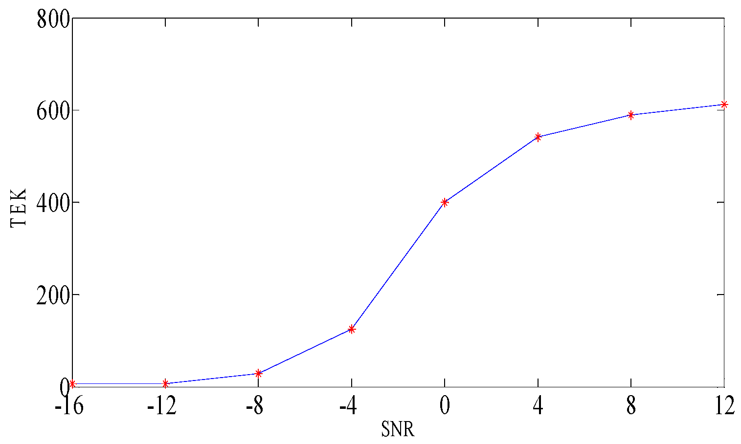
M; then, the Teager envelope spectral kurtosis (TEK) is used as the objective function to optimize the filter length L by the iterative algorithm.
Based on the above discussion, a compound fault diagnosis method based on parallel dual-Q-factor and the improved MCKD is proposed in this paper. The method combines the compound fault characteristics of rolling bearings based on frequency characteristic analysis of composite signals. The parallel dual-Q-factor sparse decomposition algorithm is proposed for the compound faults of the inner and outer race of the bearing. The non-stationary signal is decomposed into the high resonance components and low resonance components (compound fault impact component and small amount of noise). Then, the multiple periodic failures of the compound fault signal can be extracted simultaneously. In order to further isolate and extract the compound faults, the low resonance component is processed by IMCKD, which is separated and extracted according to the different fault characteristics periods.
The remainder of this paper is organized as follows. Section 2 briefly describes the theory of the parallel dual-Q-factors base sparse decomposition. Section 3 introduces the improved maximum correlation kurtosis deconvolution (IMCKD) for selecting the input parameters appropriately. Section 4 is devoted to descriptions of the proposed method. Section 5 is dedicated to description of application of the proposed method with the simulation and experiment signals. The results show the effectiveness and reliability on the compound faults decoupling diagnosis for rolling bearings.

2. The Parallel Dual-Q-Factors Bases Sparse Decomposition

The resonance property of a signal is defined by the quality factor Q, the high Q-factor base represents the continuous oscillation component, and the low Q-factor base represents the transient oscillation component. 
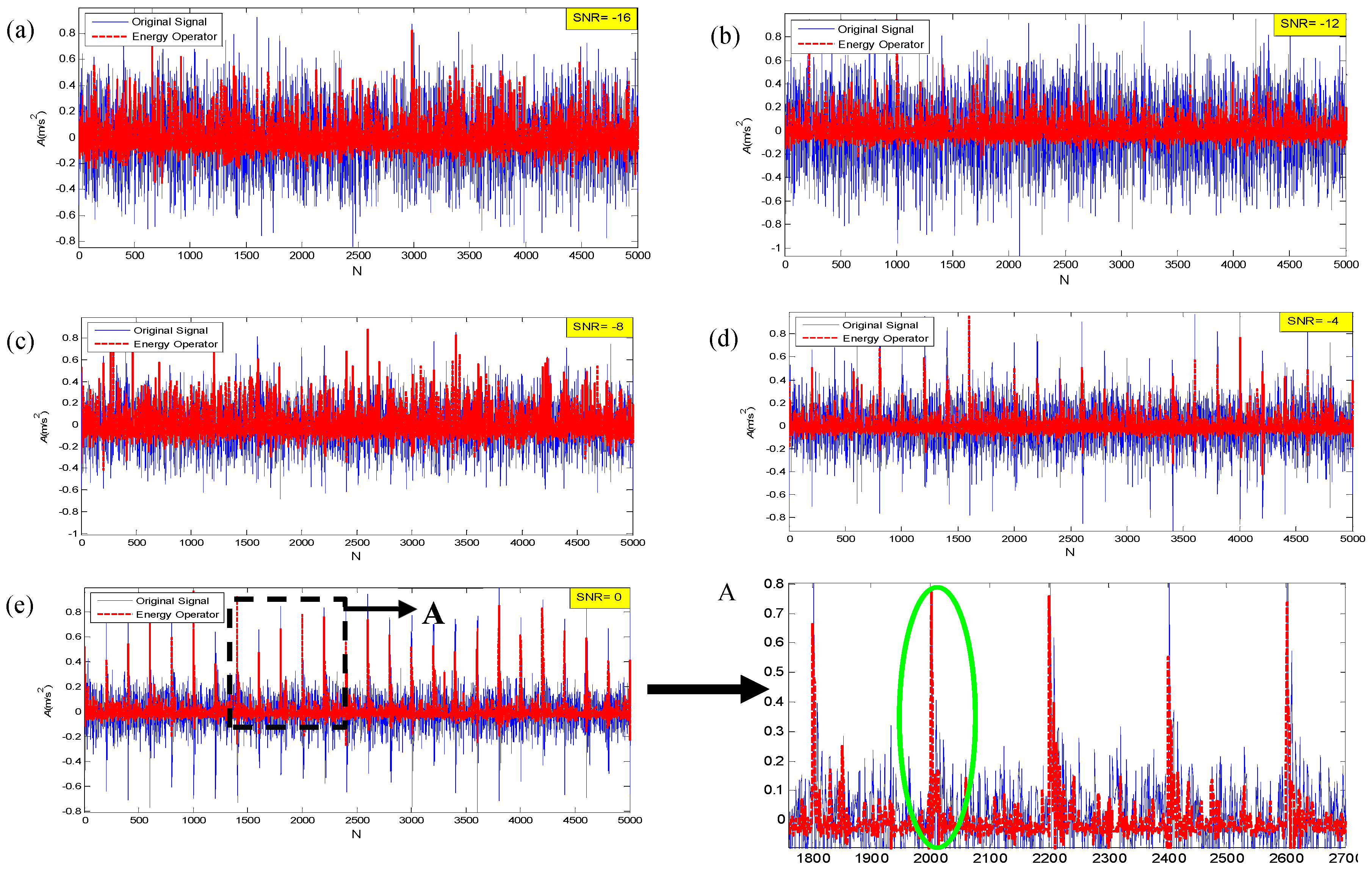
Figure 1 shows the concept of resonance properties of signals and the time-domain waveform of the signal. In Figure 1, when Q = 1, it shows the single-period pulse signal, and they are defined as the low resonance signals because of the small quality factor Q. When Q = 3 it shows the multi-period pulse signals, and they are defined as the high resonance signals because of the large quality factor Q.
The RSSD method is actually a sparse representation using the high and the low tunable Q-factor wavelet transform (TQWT) [35,38]. The TQWT is fully discrete, has the perfect reconstruction property, is modestly overcomplete, and is based on the two-channel filter bank illustrated in Figure 2 [39].
In Figure 2, x(n) is the original signal, H0(w), H1(w) and H*0(w), H*1(w) are the frequency response functions of the analysis and synthesis filters respectively; v0(n), v1(n) are the sub-band signals obtained after decomposition. y0(n), y1(n) are the synthetic signals. The scaling parameters are given by:
β = 2 Q + 1 α = 1 β r
where, β is the high-pass factor, α is the low-pass factor, and r represents the redundancy.
Suppose that the observed signal x can be represented as:
x = x 1 + x 2 x , x 1 , x 2 R N
where x1 and x2 are components with different oscillation behavior.
The signal sparse decomposition method based on the compound Q-factor basis uses the morphological component analysis (MCA) method to separate the components nonlinearly in the signal according to the oscillation characteristics [40,41] and establishes the optimal sparse representation of the high resonance component and the low resonance component. The goal of MCA is to estimate x1 and x2 individually. Assuming that the signals x1 and x2 can be sparsely represented in base functions (or frames) S1 and S2 respectively, (obtained by TQWT), they can be estimated by minimizing the objective function [42]:
J ( w 1 , w 2 ) = x S 1 W 1 S 2 W 2 2 2 + λ 1 W 1 1 + λ 2 W 2 1
where
  • W1—the transform coefficient of signal x1 under frame S1;
  • W2—the transform coefficient of signal x2 under frame S2;
  • S1—the filter banks of tunable-Q wavelet with the high quality factor;
  • S2—the filter banks of tunable-Q wavelet with the low quality factor;
  • λ1—weight parameter;
  • λ2—weight parameter.
In the sparse signal decomposition method based on the compound Q-factor bases, the objective function J is minimized through iterating and updating the coefficient W1 and W2 by using the split augmented Lagrangian searching algorithm (SALSA).
Eventually, it effectively separates the high resonance component and low resonance component, and extracts the transient impulse component. After W1 and W2 are obtained, the estimated high and low resonance components (solved by matching) are shown as follows:
x 1 ^ = S 1 W 1 * ,   x 2 ^ = S 2 W 2 * .

3. Proposed IMCKD

3.1. MCKD

The MCKD technique is based on selecting a Finite Impulse Response filter (FIR filter) to maximize the correlated kurtosis (CK), which takes advantage of the periodicity of the faults and is used to highlight the continuous pulse covered by the strong noise in the signal. Consider a discrete signal x(n) that is the response of the bearing excited by the fault impulses signal y(n). MCKD searches for a FIR filter f(l) (l is a filter length) to maximize the correlation kurtosis of the signal y ( n ) and the general expression for the inverse is given by [43]:
y ( n ) = l = 1 L f ( l ) x ( n l + 1 ) .
Correlation kurtosis is defined as an indicator in the MCKD algorithm to evaluate the impact characteristics of the resulting signal y(n) (the fault impulses signal), which can reflect the proportion of periodic influence in the signal. The correlation kurtosis is defined as [28]:
C K M ( T * ) = n = 1 N ( m = 0 M y n m T * ) 2 ( n = 1 N y n 2 ) M + 1
where M is the order of shift, L and N denote the length of filter and the sampling number of the signal respectively, f is the filter vector f = [ f 1 , f 2 , f L ] T , T * is the deconvolution period and can be calculate by the following equation:
T * = f s / f *
where f s and f * denote sampling frequency and fault characteristic frequency respectively.
The optimization function is equivalent to solving the equation:
d d f k C K M ( T ) = 0 ( k = 1 , 2 , , L ) .
The final iterative expression of the filter coefficients is represented:
f = y 2 2 β 2 ( X 0 X T 0 ) 1 m = 0 M X m T α m
where X 0 X T 0 is the Toeplitz autocorrelation matrix of the original signal x and the inverse ( X 0 X T 0 ) 1 is assumed to exist.
X r = [ x 1 r x 2 r x 3 r x N r 0 x 2 r x 3 r x N 1 r 0 0 x 3 r x N 2 r 0 0 0 x N L r + 1 ] r = [ 0   T   2 T m T ]
where
α m = [ y 1 1 m T   ( y 2 1 y 2 1 T y 2 1 M T ) y 1 2 m T   ( y 2 2 y 2 2 T y 2 2 M T ) y 1 N m T ( y 2 N y 2 N T y 2 N M T ) ] β = [ y 1 y 1 T     y 1 M T y 2 y 2 T     y 2 M T y N y N T y N M T ] .
The performance of MCKD must be guaranteed by the accurate and appropriate parameters, the input parameters, including the length of filter L, the order of shift M, the maximum count of iteration N and the deconvolution period T * .
(1) Generally, the maximum count of iteration N is empirically set. The larger count of iteration may bring a better result when the algorithm is executed to convergence but needs more calculation time. Therefore, to ensure the algorithms converge in this paper, N = 30 is set as the maximum count of iteration in MCKD [37].
(2) The deconvolution period T * is obtained from the theoretical fault characteristic frequency mentioned above.
(3) The optimal M and L are different when MCKD is applied in different signal. Obviously, the main problem in the practical application of MCKD is how to select the optimal parameters including the order of shift M and the filter length L.

3.2. IMCKD

When the four parameters are determined appropriately, which contains the length of filter L, the order of shift M, the maximum count of iteration N and the deconvolution period T * , the MCKD technique can select a FIR filter to maximize the correlated kurtosis (CK). Then, the fault impulse signal y ( n ) is obtained by deconvolution of the original input signal x ( n ) with this filter. Finally, the periodic impulse faults component is separated out from the vibration signal.
In order to select the best shift order M and the filter length L for MCKD in all cases, and ensure the effectiveness of MCKD for extracting the fault features from the vibration signal, the improved maximum correlation kurtosis deconvolution (IMCKD) is proposed. When the signal is deconvoluted and filtered with the optimal parameters by MCKD, the signal noise reduction effect is very good. The Teager envelope spectral kurtosis (TEK) value can measure the noise reduction effect, and reflect the degree of signal to noise ratio, so the TEK value of the impulse signal y ( n ) is used as the evaluation criterions to benefit for selecting the MCKD parameters.

3.2.1. The Index Teager Envelope Spectral Kurtosis (TEK)

The Teager energy operator (TEO) is a nonlinear operator proposed by Kaiser that can effectively extract the energy of the signal, which can effectively highlight the transient characteristics of the impact component [44]. The Teager energy operator is used to track the instantaneous energy of signal y ( t ) , which is defined as follows [45]:
y n ¯ ( t ) = ψ [ y n ( t ) ] = y ˙ n 2 ( t ) y n ( t ) y ¨ n ( t )
where, y ˙ ( t ) and y ¨ ( t ) are the first and second derivatives of the signal y ( t ) .
We simulated the bearing single point fault signal and added random noise with Signal to Noise Ratio (SNR) of −16, −12, −8, −4, 0, 4, 8, 12 (dB) respectively. Then we calculated the Teager energy operator signal using Equation (11), and the results are shown in Figure 3.
The blue line represents the original signal and the red line represents the Teager energy operator signal, and A, B represent the partial enlargements of SNR = 0 and SNR = 8 dB, respectively. It can be seen from Figure 3 that TEO can track the instantaneous energy of the signal and better reflect the impact characteristics from the time-domain partial map.
Then, we calculated their envelope spectrum by Hilbert transform by the following equation:
E ( t ) = y ¯ n 2 ( t ) + ( 1 π y ¯ n ( τ ) t τ d τ ) 2
and calculated their envelope spectral kurtosis (TEK):
T E K = 1 / N i = 1 N ( E i ( t ) u E ) 4 [ 1 / N i = 1 N ( E i ( t ) u E ) 2 ] 2
where u E is the mean of the signal and N is the signal length. The corresponding TEK values for different SNRs are shown in the Figure 4.
It can be seen from the trend graph that as the SNR of the signal increases, the TEK value tends to increase. Therefore, the index TEK can be used to measure the noise reduction effect of the signal.

3.2.2. The Optimal Selection of M and L

The general procedure of the optimization selection for M and L is as follows:
Step 1: Mj = j, set the scope [1,7] for j, when M > 7. This iterative method will reduce the accuracy of the calculation because it exceeds the range of the floating-point index. Li = i, set the scope [5,350] for i;
Step 2: Calculate T * = T O = f s / f o from Equation (7), when f * is f o ;
Step 3: When j = 1, M 1 = 1 , Li = i = [5, 6, …, 350] substitute into the MCKD algorithm respectively; then, the corresponding 346 fault impulse signals y i ( n ) o u t e r ( i = [ 5 , , 350 ] ) are obtained; next, calculate the TEK of each fault impulse signal; finally, calculate the mean of TEK values (MTEK), i.e., M T E K 1 outer . Similarly, for each of M j ( j = [ 1 , 2 , , 7 ] ) , calculate M T E K 2 outer , M T E K 3 outer , …, M T E K 7 outer ;
Step 4: Select Mj for the best shift order Mbest-o when MTEKj-outer is the largest;
Step 5: When T * = T O , M = M b e s t o , Li = i = [5, 6, …, 350] substitute into the MCKD algorithm respectively, corresponding 346 fault impulse signals y i ( n ) o u t e r ( i = [ 5 , , 350 ] ) are obtained, then calculate the TEK of each fault impulse signal, i.e., T E K i outer ( i = [ 5 , 6 , , 350 ] ) ;
Step 6: Select Li for the best shift order Lbest-o when TEKi-outer is the largest;
Step 7: Calculate T * = T i = f s / f i from Equation (7), when f * is f i ;
Step 8: Obtain M b e s t i and Lbest-I by repeating step 3–6.

4. Procedure of Compound Faults Diagnosis

This method is applied to separate and extract the compound fault of the inner and outer race of the bearing. Firstly, the input measured signal is preprocessed by the parallel dual-Q-factor base sparse decomposition to obtain a low resonance component, and the compound failure impacts of the inner and outer rings are clearly extracted. Then the IMCKD is used to separate and extract the compound fault feature according to different fault periods. The specific process of the proposed method is illustrated in the flow chart shown in Figure 5, and the method is described as follows:
(1)
Input the vibration signal x(t), including noise, random vibration generated by normal parts of the rolling bearing and shock vibration generated by composite faults.
(2)
Use the parallel dual-Q-factor bases sparse decomposition to obtain the high resonance components (random vibration generated by the normal part and strong noise) and the low resonance components (composite fault impact component and a small amount of noise):
  • Set the appropriate decomposition parameters: The quality factor Q1, Q2, the redundancy r1, r2, and the number of layers J1, J2;
  • Decompose the input signal x(t) using the parallel dual-Q-factor;
  • Extract the low resonance component xL;
(3)
The low resonance components of the signal are deconvoluted and filtered with the optimal parameters by IMCKD:
  • Calculate the T * (* is i, o; i represents inner, o represents outer), and pre-select the scope of MCKD parameters (M, L);
  • Calculate M b e s t i , Lbest-i and M b e s t o , Lbest-o based on Section 3.2.2;
  • The low resonance component xL is deconvoluted and filtered with the optimized parameters [To, M b e s t o , Lbest-o] and [Ti, M b e s t i , Lbest-i] respectively to obtain the time domain signals y1 and y2;
(4)
Extract the fault feature frequency from the envelope spectrum calculated by Hilbert Transform (HT).

5. Application of the Proposed Method

To verify the effectiveness of the proposed method for extracting the fault characteristic components in the noise, this method has been applied to simulation analysis and experimental cases.

5.1. Simulation Analysis

5.1.1. The Construction of Compound Fault Simulation Signal

The compound fault signal was simulated by the simulation signal of the inner race and outer race. The outer race fault signal simulation model was defined as in the following equation [46]:
x 0 ( t ) = y 0 e ( 2 ζ π f n t 0 ) sin ( 2 π f n 1 ζ 2 t 0 )
where y 0 is the possible amplitude modulator; f n is the natural frequency; t 0 is a single cycle sampling time; ζ is the damping factor. The parameters of the outer race simulation signal are shown in Table 1.
The inner race fault simulation signal is defined as:
x i ( t ) = s ( t ) + n ( t ) = i A i h ( t i T τ i ) + n ( t )
where
A i = A 0 cos 2 ( 2 π f r t + ϕ A ) + C A h ( t ) = e B t cos ( 2 π f n t + ϕ ω ) 1 / f r
where τ i represents the minor fluctuation of the i shock relative to the period T; A i is the amplitude modulation with 1 / f r as a cycle; ℎ(t) is an exponential decay pulse; B is the attenuation coefficient of the system; ϕ A , ϕ ω are the initial phase. The parameters of the inner race simulation signal are shown in Table 2.
The mathematical model of the compound inner race and outer race spalling is shown in Equation (18):
x ( t ) = x i ( t ) + x 0 ( t ) .
The time domain waveform of the outer race and inner race fault simulation signals are shown in Figure 6a,b. Figure 7a is the compound signal; Figure 7b is the compound fault simulation signal with gauss noise. It can be seen from Figure 7b that the inner and outer periodic shock characteristics are overwhelmed by noise and it cannot accurately reflect the characteristics of fault impact. Therefore, it is necessary to further extract fault features.

5.1.2. Compound Faults Feature Extraction for Simulation Signal

Firstly, the sparse decomposition of the parallel dual-Q-factor bases is applied to extract and sparsely represent the compound fault components according to the proposed method. The decomposition parameters are shown in Table 3, and the analysis results are shown in Figure 8. Figure 8a,b are the low resonance components which is obtained by using the sparse decomposition method and the Hilbert envelope spectra of decomposed components respectively. It can be seen from Figure 8b that peaks are obvious at fr (24.38 Hz), fo (61.88 Hz), fi (300 Hz) and their harmonics. Hence, the results indicate that the method can successfully identify and extract features of the simulated signal composed of impact components of the inner race and outer race simultaneously. However, the two fault impact signals are overlapped with each other, and the two fault characteristic frequencies and their harmonics are interlaced with each other. Therefore, it is difficult to accurately extract the two-fault characteristic information from the envelope spectrum.
To further separate the inner and outer race fault features from the composite fault signals, according to the different fault periods of the inner and outer race of the rolling bearing, the adaptable deconvolution techniques was applied to extract the periodic features from the low resonance component. The deconvolution period T * (* is i, o) of the signal is shown in Table 4.
Then, we selected the optimal parameter (M, L) as mentioned in Section 3.2.2
(1) When To = 248, Figure 9a,b show the relationship between M and MTEK, and the relationship between the filter length L and the TEK by iterative calculation respectively. It was found that when M = 3, the MTEK value was the largest from Figure 9a, and when L = 20, the TEK value was the largest from Figure 9b, so the optimal parameters To, Mo, and Lo were determined [248, 3, 20].
(2) When Ti = 51, Figure 9c,d show the relationship between M and MTEK, and the relationship between the filter length L and the TEK by iterative calculation respectively. It was found that when M = 5, the MTEK value was the largest from Figure 9c, and when L = 55, the TEK value was the largest from Figure 9d, so the optimal parameters Ti, Mi, and Li were determined [51, 5, 55].
The low resonance component was deconvoluted and filtered with the obtained optimal parameters [T*, M*, L*] (* is i, o) using MCKD. Finally, the analysis result is presented in Figure 10. It is noticeable that the impulse components in the time-domain of the outer race fault and the inner race fault can be found clearly in Figure 10a,c, respectively. From Figure 10b,d, the harmonic components of the characteristic frequencies of 61.88 Hz and 300 Hz are revealed noticeably. It is consistent with the theoretical fault characteristic frequency (fo (62 Hz), fi (300 Hz)). The results indicate that the proposed method can successfully separate the features of the simulated signal composed of the outer race fault and the inner race fault.

5.2. Experimental Verification

Figure 11 and Figure 12 shows the test rig to collect the vibration data of the bearing. The test rig consisted of a motor driving the shaft through a flexible coupling, HG3528A data collection instrument and laptop. The vibration acceleration of the damaged bearing in the vertical planes were measured using an accelerometer, the bearing model was SKF6307. The output from the accelerometer was sampled at 15360 Hz. The motor was run at 1496 rpm, and the collected data was uploaded to the laptop for data processing and analysis.
The bearing with compound fault (Figure 13) was machined as a pitting defect on the outer race and inner race of the bearing with the size of 1 mm in diameter and 0.2 mm in depth. The fault characteristic frequencies of the outer race and inner race were fo = 76.7 Hz and fi = 122.7 Hz respectively.
The experimental data of the compound fault was selected for analysis. The time-domain signal and the frequency spectrum are shown in Figure 14. The impact components in the graph were not obvious, so the fault features needed to be further extracted.
The sparse decomposition of the parallel dual-Q-factor bases was applied to extract and sparsely represent the compound fault components. The decomposition parameters are shown in Table 5, and the analysis results are shown in Figure 15. Figure 15a,b are the low resonance components which were obtained by using the sparse decomposition method and the Hilbert envelope spectra of decomposed components respectively. It can be seen from Figure 15b that peaks were obvious at fo (76.88 Hz), fi (121.9 Hz) and their harmonics. Hence, the results indicate that the proposed method can identify and extract features of the compound impact components of the inner race and outer race simultaneously. However, the two fault impact signals are overlapped with each other, and the two fault characteristic frequencies and their harmonics are interlaced with each other. Therefore, it is difficult to accurately extract the two-fault characteristic information from the envelope spectrum.
To further separate the inner and outer race fault features from the composite fault signals, the improved deconvolution techniques were applied to extract the periodic features from the low resonance component. The deconvolution period T * (* is i, o) of the signal is shown in the Table 6.
Then, we selected the optimal parameter (M, L) as mentioned in Section 3.2.2
(1) When To=200, Figure 16a,b show the relationship between M and MTEK, and the relationship between the filter length L and the TEK by iterative calculation respectively. It was found that when M = 1, the MTEK value was the largest from Figure 16a, and when L = 260, the TEK value was the largest from Figure 16b, so the optimal parameters To, Mo, and Lo were determined [200, 1, 260].
(2) When Ti = 125, Figure 16c,d show the relationship between M and MTEK, and the relationship between the filter length L and the TEK by iterative calculation respectively. It was found that when M = 6, the MTEK value was the largest from Figure 16c, and when L = 250, the TEK value was the largest from Figure 16d, so the optimal parameters Ti, Mi, and Li were determined [125, 6, 250].
The low resonance component was deconvoluted and filtered with the obtained optimal parameters [T*, M*, L*] (* is i, o) using MCKD. Finally, the analysis result is presented in Figure 17. It was noticeable that the impulse components in the time-domain of outer race fault and inner race faults were found clearly in Figure 17a,c respectively. From Figure 17b,d, the harmonic components of the characteristic frequencies 76.88 Hz and 121.9 Hz were revealed noticeably. It is consistent with the theoretical fault characteristic frequency (fo (76.7 Hz), fi (122.7 Hz)). The results show that the proposed method successfully separated the fault information of the outer race and inner race of the bearing from the composite fault signal.

6. Conclusions

The failure of a rolling bearing usually manifests itself as compound failure, which are coupled with each other. The fault characteristic frequencies in the envelope spectrum are staggered with each other, so it is difficult to accurately separate them. This study presents a compound fault diagnosis method for rolling bearings based on a parallel dual-Q-factor and the improved maximum correlated kurtosis deconvolution (IMCKD). The parallel dual-Q-factor bases sparse decomposition is used as noise reduction processing. Improving the MCKD according to the index TEK can reflect the noise reduction effect, which can select the appropriate parameters of MCKD, and accurately realize the separation and extraction of composite fault features. After the composite fault signal is filtered and de-noised by this method, the spectrum peak of the fault feature frequency and its harmonics are clearly presented in the spectrum diagram, which is basically consistent with the theoretical calculation value. Therefore, it is possible to recognize the inner and outer race faults. The effectiveness of the proposed method is verified by analyzing the compound fault mathematical simulation signal and the measured signal. The characters of compound faults are the multiplicity of faults, which brings great difficulties for fault diagnosis, so more study should be conducted on compound fault detection in the future.

Author Contributions

L.C. and J.D., conceived and designed the method, N.Y. was responsible for the subject revision, and Y.X. and L.S. analyzed the data. All authors have read and approved the final manuscript.

Funding

Funding was provided by the National Natural Science Foundation of China (Grant No. 51575007).

Acknowledgments

The authors would like to appreciate anonymous reviewers and editors for their valuable comments and constructive suggestions.

Conflicts of Interest

The authors declare no conflict of interest.

References

  1. Song, L.; Wang, H.; Chen, P. Step-by-step Fuzzy Diagnosis Method for Equipment Based on Symptom Extraction and Trivalent Logic Fuzzy Diagnosis Theory. IEEE Trans. Fuzzy Syst. 2018, 26, 3467–3478. [Google Scholar] [CrossRef]
  2. Shen, C.Q.; Qi, Y.M.; Wang, J.; Cai, G.G.; Zhu, Z.K. An automatic and robust features learning method for rotating machinery fault diagnosis based on contractive autoencoder. Eng. Appl. Artif. Intell. 2018, 76, 170–184. [Google Scholar] [CrossRef]
  3. Cui, L.; Wang, X.; Xu, Y.G.; Jiang, H.; Zhou, J.P. A novel Switching Unscented Kalman Filter method for remaining useful life prediction of rolling bearing. Measurement 2019, 135, 678–684. [Google Scholar] [CrossRef]
  4. Han, T.; Jiang, D.; Zhao, Q.; Wang, L.; Yin, K. Comparison of random forest, artificial neural networks and support vector machine for intelligent diagnosis of rotating machinery. Trans. Inst. Meas. Control. 2018, 40, 2681–2693. [Google Scholar] [CrossRef]
  5. Li, C.; de Oliveira, J.L.V.; Lozada, M.C.; Cabrera, D.; Sanchez, V.; Zurita, G. A systematic review of fuzzy formalisms for bearing fault diagnosis. IEEE Trans. Fuzzy Syst. 2019. [Google Scholar] [CrossRef]
  6. Wang, H.; Li, S.; Song, L.Y.; Cui, L. A novel convolutional neural network based fault recognition method via image fusion of multi-vibration-signals. Comput. Ind. 2019, 105, 182–190. [Google Scholar] [CrossRef]
  7. Zhang, B.; Zhang, S.; Li, W. Bearing performance degradation assessment using long short-term memory recurrent network. Comput. Ind. 2019, 106, 14–29. [Google Scholar] [CrossRef]
  8. Cui, L.; Wang, J.; Lee, S. Matching Pursuit of an Adaptive Impulse Dictionary for Bearing Fault Diagnosis. JSV 2014, 333, 2840–2862. [Google Scholar] [CrossRef]
  9. Zhang, X.; Liu, Z.; Miao, Q. Bearing fault diagnosis using a whale optimization algorithm-optimized orthogonal matching pursuit with a combined time–frequency atom dictionary. MSSP 2018, 107, 29–42. [Google Scholar] [CrossRef]
  10. Cui, L.L.; Yao, T.C.; Zhang, Y.; Gong, X.Y.; Kang, C.H. Application of pattern recognition in gear faults based on the matching pursuit of a characteristic waveform. Measurement 2017, 104, 212–222. [Google Scholar] [CrossRef]
  11. Wang, H.Q.; Ren, B.Y.; Song, L.Y.; Cui, L.L. A Novel Weighted Sparse Representation Classification Strategy based on Dictionary Learning for Rotating Machinery. IEEE Trans. Instrum. Meas. 2019. [Google Scholar] [CrossRef]
  12. Cui, L.; Li, B.; Ma, J.F.; Jin, Z. Quantitative trend fault diagnosis of a rolling bearing based on Sparsogram and Lempel-Ziv. Measurement 2018, 128, 410–418. [Google Scholar] [CrossRef]
  13. Li, X.; Yu, K.; Ma, H.; Cao, L.; Luo, Z.T.; Li, H.F.; Che, L.Y. Analysis of varying contact angles and load distributions in defective angular contact ball bearing. Eng. Fail. Anal. 2018, 91, 449–464. [Google Scholar] [CrossRef]
  14. Cui, L.; Jin, Z.; Huang, J.F.; Wang, H.Q. Fault severity classification and size estimation for ball bearings based on vibration mechanism. IEEE Access 2019. [CrossRef]
  15. Song, L.Y.; Wang, H.; Chen, P. Vibration-Based Intelligent Fault Diagnosis for Roller Bearings in Low-Speed Rotating Machinery. IEEE Trans. Instrum. Meas. 2018, 67, 1887–1899. [Google Scholar] [CrossRef]
  16. Cui, L.; Huang, J.F.; Zhang, F.B. HVSRMS localization formula and localization law: Localization diagnosis of a ball bearing outer ring fault. MSSP 2019, 120, 608–629. [Google Scholar] [CrossRef]
  17. Chen, L.J. Compound faults detection of rotating machinery using improved adaptive redundant lifting multiwavelet. MSSP 2013, 38, 36–54. [Google Scholar] [CrossRef]
  18. Li, C.; Mariela, C.; Cabrera, D.; Sanchez, R.V.; Pacheco, F.; Ulutagay, G.; Valente de Oliveira, J. Ulutagay and José Valente de Oliveira, A comparison of fuzzy clustering algorithms for bearing fault diagnosis. JIFS 2018, 34, 3565–3580. [Google Scholar]
  19. Wang, W.J.; Cui, L.L.; Chen, D.Y. Multi-scale morphology analysis of acoustic emission signal and quantitative diagnosis for bearing fault. Acta Mech. Sin. 2016, 32, 265–272. [Google Scholar] [CrossRef]
  20. Jiang, Y.; Zhu, H.; Li, Z. A new compound faults detection method for rolling bearings based on empirical wavelet transform and chaotic oscillator. Chaos Solitons Fractals 2016, 89, 8–19. [Google Scholar] [CrossRef]
  21. Luo, M.; Li, C.S.; Zhang, X.Y. Compound feature selection and parameter optimization of elm for fault diagnosis of rolling element bearings. ISA Trans. 2016, 65, 556–566. [Google Scholar] [CrossRef] [PubMed]
  22. Hao, Y.; Song, L.; Cui, L.; Wang, H. A three-dimensional geometric features-based SCA algorithm for compound faults diagnosis. Measurement 2019, 134, 480–491. [Google Scholar] [CrossRef]
  23. Tang, G.; Luo, G.; Zhang, W.; Yang, C.; Wang, H. Underdetermined Blind Source Separation with Variational Mode Decomposition for Compound Roller Bearing Fault Signals. Sensors 2016, 16. [Google Scholar] [CrossRef] [PubMed]
  24. Hao, Y.S.; Song, L.; Wang, M.Y.; Cui, L.; Wang, H. Underdetermined Source Separation of Bearing Faults Based on Optimized Intrinsic Characteristic-Scale Decomposition and Local Non-Negative Matrix Factorization. IEEE Access 2019, 7, 11427–11435. [Google Scholar] [CrossRef]
  25. Huang, R.; Liao, Y.; Zhang, S.; Li, W. Deep Decoupling Convolutional Neural Network for Intelligent Compound Fault Diagnosis. IEEE Access 2019, 7, 1848–1858. [Google Scholar] [CrossRef]
  26. Hao, Y.; Song, L.; Ke, Y.; Wang, H.; Chen, P. Diagnosis of Compound Fault Using Sparsity Promoted-Based Sparse Component Analysis. Sensors 2017, 17, 1307. [Google Scholar] [CrossRef]
  27. Antoni, J. Blind separation of vibration components: Principles and demonstrations. MSSP 2005, 19, 1166–1180. [Google Scholar] [CrossRef]
  28. Mcdonald, G.L.; Zhao, Q.; Zuo, M.J. Maximum correlated Kurtosis deconvolution and application on gear tooth chip fault detection. MSSP 2012, 33, 237–255. [Google Scholar] [CrossRef]
  29. Sun, P.; Liao, Y.; Lin, J. The Shock Pulse Index and Its Application in the Fault Diagnosis of Rolling Element Bearings. Sensors 2017, 17, 535. [Google Scholar] [CrossRef]
  30. Hong, L.; Dhupia, J.S. A time domain approach to diagnose gearbox fault based on measured vibration signals. JSV 2014, 333, 2164–2180. [Google Scholar] [CrossRef]
  31. Feng, J.; Lei, Y.; Shan, H. Early Fault Diagnosis of Bearings Using an Improved Spectral Kurtosis by Maximum Correlated Kurtosis Deconvolution. Sensors 2015, 15, 29363–29377. [Google Scholar]
  32. Wang, H.; Wang, P.X.; Song, Y.L.; Ren, B.Y.; Cui, L. A Novel Feature Enhancement Method based on Improved Constraint Model of Online Dictionary Learning. IEEE Access 2019, 7, 17599–17607. [Google Scholar] [CrossRef]
  33. Jiang, X.X.; Shen, C.Q.; Shi, J.J.; Zhu, Z.K. Initial center frequency-guided VMD for fault diagnosis of rotating machines. Sound Vib. 2018, 435, 36–55. [Google Scholar] [CrossRef]
  34. Cui, L.; Wang, X.; Wang, H.; Wu, N. Improved Fault Size Estimation Method for Rolling Element Bearings Based on Concatenation Dictionary. IEEE Access 2019, 7, 22710–22718. [Google Scholar] [CrossRef]
  35. Selesnick, I.W. Wavelet Transform with Tunable Q-Factor. IEEE Trans. Signal Process. 2011, 59, 3560–3575. [Google Scholar] [CrossRef]
  36. Cai, G.G.; Chen, X.F.; He, Z.J. Sparsity-enabled signal decomposition using tunable Q-factor wavelet transform for fault feature extraction of gearbox. MSSP 2013, 41, 34–53. [Google Scholar] [CrossRef]
  37. Wang, H.P.; Chen, B.Q.; Zeng, N.Y. Sparsity-based signal extraction using dual Q-factors for gearbox fault detection. ISA Trans. 2018, 79, 147–160. [Google Scholar] [CrossRef]
  38. Chen, B.J.; Shen, B.M.; Chen, F.F. Fault diagnosis method based on integration of RSSD and wavelet transform to rolling bearing. Measurement 2019, 131, 400–411. [Google Scholar] [CrossRef]
  39. Zhang, D.C.; Yu, D.J.; Li, X. Optimal resonance-based signal sparse decomposition and its application to fault diagnosis of rotating machinery. Inst. Mech. Eng. 2017, 231, 4670–4683. [Google Scholar] [CrossRef]
  40. Bobin, J.; Starck, J.L. Morphological component analysis: An adaptive thresholding strategy. IEEE Trans Image Process. 2007, 16, 2675–2681. [Google Scholar] [CrossRef]
  41. Luo, G.; Wang, H. Diagnosis of rolling element bearing fault a rising in gearbox based on sparse morphological component analysis. J. Vibroeng. 2017, 19, 189–203. [Google Scholar] [CrossRef]
  42. Zhang, D.C.; Yu, D.J.; Zhang, W.Y. Energy operator demodulating of optimal resonance components for the compound faults diagnosis of gearboxes. Meas. Sci. Technol. 2015, 26, 115003. [Google Scholar] [CrossRef]
  43. Miao, Y.H.; Zhao, M.; Lin, J.; Lei, Y.G. Application of an improved maximum correlated kurtosis deconvolution method for fault diagnosis of rolling element bearings. MSSP 2017, 92, 173–195. [Google Scholar] [CrossRef]
  44. Kedadouche, M.; Thomasa, M. A hybrid method combining Teager Kaiser energy operator, empirical mode decomposition and minimum entropy deconvolution for monitoring gears damages. Mech. Ind. 2015, 16, 1. [Google Scholar] [CrossRef]
  45. Maragos, P.; Kaiser, J.F. On amplitude and frequency demodulation using energy operators. IEEE Trans. Signal Process. 1993, 41, 1532–1550. [Google Scholar] [CrossRef]
  46. Wan, S.T.; Zhou, X.; Dou, L.J. Compound Fault Diagnosis of Bearings Using an Improved Spectral Kurtosis by MCDK. Math. Probl. Eng. 2018. [Google Scholar] [CrossRef]
Figure 1. The time-domain diagram of low Q-factor and high Q-factor.
Applsci 09 01681 g001
Figure 2. Analysis and synthesis filter banks for the dual-Q wavelet transform.
Applsci 09 01681 g002
Figure 3. The diagram of Teager energy operator under different SNRs, (a) −16 dB, (b) −12 dB, (c) −8 dB, (d) −4 dB, (e) 0 dB, (f) 4 dB, (g) 8 dB, (h) 12 dB. A—the partial enlargements of (e); B—the partial enlargements of (f).
Applsci 09 01681 g003aApplsci 09 01681 g003b
Figure 4. The Teager envelope spectral kurtosis (TEK) values for different SNRs.
Applsci 09 01681 g004
Figure 5. The flow chart of the proposed method.
Applsci 09 01681 g005
Figure 6. The time-domain waveform of the single fault simulation signal: (a) Outer race; (b) Inner race.
Applsci 09 01681 g006
Figure 7. The time-domain waveform of the compound fault simulation signal: (a) Outer race and inner race fault; (b) compound signal with gauss noise.
Applsci 09 01681 g007
Figure 8. The analysis results of case 1 with the parallel dual-Q-factor bases sparse decomposition: (a) Low resonance component; (b) Hilbert envelope spectrum.
Applsci 09 01681 g008
Figure 9. The variation curves of MTEK and TEK for case 1: (a) To = 248, the tendency of MTEK with M; (b) To = 248, the iterative result between L and TEK; (c) Ti = 51, the tendency of MTEK with M; (d) Ti = 51, the iterative result between L and TEK.
Applsci 09 01681 g009
Figure 10. The analyzed results of case 1 with the proposed method: (a) To = 248, low resonance component; (b) To = 248, Hilbert envelope spectrum; (c) Ti = 51, low resonance component; (d) Ti = 51, Hilbert envelope spectrum.
Applsci 09 01681 g010
Figure 11. Schematic diagram of the experimental bench system: ① Three-phase asynchronous motor; ② flexible shaft coupling; ③ the bearing with compound fault; ④ bearing rotor; ⑤ the normal bearing.
Applsci 09 01681 g011
Figure 12. The experimental bench system.
Applsci 09 01681 g012
Figure 13. The bearing with compound fault.
Applsci 09 01681 g013
Figure 14. Compound fault vibration signal and its frequency spectrum.
Applsci 09 01681 g014
Figure 15. The analysis results of case 2 with the parallel dual-Q-factor bases sparse decomposition: (a) Low resonance component; (b) envelope spectrum.
Applsci 09 01681 g015
Figure 16. The variation curves of MTEK and TEK for case 2: (a) To = 200, the tendency of MTEK with M; (b) To = 200, the TEK result for outer race; (c) Ti = 125, the tendency of MTEK with M; (d) Ti = 125, the TEK result for outer race.
Applsci 09 01681 g016aApplsci 09 01681 g016b
Figure 17. The analyzed results of case 2 with the proposed method: (a) To = 200, low resonance component; (b) To = 200, Hilbert envelope spectrum of (a); (c) Ti = 125, low resonance component; (d) Ti = 125, Hilbert envelope spectrum of (c).
Applsci 09 01681 g017
Table 1. The parameters of outer fault simulation signal.
Rotating Frequency fr /HzNatural Frequency fn /HzSampling Frequency fs /HzSampling Point NFault Frequency fo /Hz
24200015360819262
Table 2. The parameters of inner fault simulation signal.
Rotating Frequency fr /HzNatural Frequency fn /HzSampling Frequency fs /HzSampling Point NFault Frequency fi /Hz
242000153608192300
Table 3. The sparse decomposition parameters of case 1.
AttributeQ1, Q2Redundancy (r1, r2)Number of Layers (J1, J2)
Low resonance component1427
High resonance component6412
Table 4. The parameters T* (* is i, o).
Fault TypeFault FrequencyPeriod of Interest T* (* is i, o)
Outer racefo (62 Hz)To = 248
Inner racefi (300 Hz)Ti = 51
Table 5. The sparse decomposition parameters of case 2.
AttributeQ1, Q2Redundancy (r1, r2)Number of Layers (J1, J2)
Low resonance component1425
High resonance component6611
Table 6. The parameters T* (* is i, o).
Fault TypeFault FrequencyPeriod of Interest T* (* is i, o)
Outer racefo (76.7 Hz)To = 200
Inner racefi (122.7 Hz)Ti = 125

