Medical Image Segmentation with Adjustable Computational Complexity Using Data Density Functionals

Featured Application

The research work proposes an avenue of image segmentation that can simultaneously reduce computational complexity and filter image pollution for clinical investigations.

Abstract

Techniques of automatic medical image segmentation are the most important methods for clinical investigation, anatomic research, and modern medicine. Various image structures constructed from imaging apparatus achieve a diversity of medical applications. However, the diversified structures are also a burden of contemporary techniques. Performing an image segmentation with a tremendously small size (<25 pixels by 25 pixels) or tremendously large size (>1024 pixels by 1024 pixels) becomes a challenge in perspectives of both technical feasibility and theoretical development. Noise and pixel pollution caused by the imaging apparatus even aggravate the difficulty of image segmentation. To simultaneously overcome the mentioned predicaments, we propose a new method of medical image segmentation with adjustable computational complexity by introducing data density functionals. Under this theoretical framework, several kernels can be assigned to conquer specific predicaments. A square-root potential kernel is used to smoothen the featured components of employed images, while a Yukawa potential kernel is applied to enhance local featured properties. Besides, the characteristic of global density functional estimation also allows image compression without losing the main image feature structures. Experiments on image segmentation showed successful results with various compression ratios. The computational complexity was significantly improved, and the score of accuracy estimated by the Jaccard index had a great outcome. Moreover, noise and regions of light pollution were mostly filtered out in the procedure of image compression.

1. Introduction

Automatic identification and segmentation of medical imageries benefit the planning and guidance of modern surgery [1,2,3,4,5], clinical investigations [6,7,8,9,10], rehabilitation [11,12,13], and so forth. High-quality reconstructive anatomical morphology provides convenience on surgery planning and the understanding between organ functionalities and pathological diagnosis. The corresponding investigations regarding neural circuitries of human brains also provide constructive consequences on research progress of connectome [14] and clinical diagnoses related to Alzheimer’s and Parkinson’s diseases [15]. Thus, among these applications, robust automatic methods of segmentation for large-scale medical imageries can efficiently save extensive and tedious manual interventions while dealing with humongous tissue labeling and clinical process setting. Among those developed techniques, state-of-the-art methodologies on the field of magnetic resonance image (MRI) processing successfully combined several merits from interdisciplinary methods [16,17,18] and exhibit an opportunity to track brain regions related to relevant diseases [19,20]. For instance, precise identification and segmentation of subthalamic nucleus from three-dimensional medical imageries facilitate the automatic planning of deep brain stimulation, and the clinical result has also shown clinical potential for relieving the motor symptoms of advanced Parkinson’s disease [8,21,22].

The automatic segmentation methods often can only have commonplace performance when there is a large ratio of the whole image size to the size of the desired tissue area. The tiny desired tissue area within an image and the poorly defined boundaries between the desired tissue area and its neighboring regions limit the feasibility of segmentation methods. For instance, since there is a large ratio of the whole brain tissue to the subthalamic nucleus, the image segmentation of the tiny subthalamic nucleus (approximately 6 mm × 4 mm × 5 mm) from their neighboring regions such as putamen, substantia nigra, zona incerta, and so forth [23], is always an open problem for the clinical investigations of deep brain stimulation. Besides, the contemporary MRI techniques for identification and localization of brain tissues, such as T2-weighted-imaging [24,25], susceptibility weighted imaging [26,27,28], fluid-attenuated inversion recovery [29,30,31], and so on, often fail to distinguish desired minuscule tissues from their surrounding structures in clinical MRI processes. Furthermore, the anatomical information regarding the tiny tissues is only caught in few MR images during the acquirement processes. For physically localizing the subthalamic nucleus in the procedure of deep brain stimulation, a compensation method is to utilize the technique of intraoperative microelectrode recording to extract electric signal differences between the subthalamic nucleus and its neighboring regions. However, this method requires significant neurosurgical expertise and lengthens the surgery duration [8,23]. Therefore, to solve these essential problems in medical applications, the adopted methods should focus on the identification and the localization of the tiny desired anatomical tissues and their surrounding regions by only utilizing the information acquired from medical images. Meanwhile, to reduce extensive and tedious manual interventions and for the convenience of visualization, the applied method should execute artificial intelligence approaches for automatically achieving the goals of image segmentation and pattern recognition. Considering the preprocessing of the medical imageries on data compression and denoising would be valuable for large-scale medical images to pursue further execution efficiency [11,12,32].

To resolve the issues of image compression, state-of-the-art techniques based on the frameworks of wavelet transform [33,34,35,36,37] and neural networks [38,39,40,41,42,43,44] in probabilistic perspectives have brought about their fruitful achievements. The wavelet-transform-based techniques usually use a specific wavelet technique based on the Mallat filter [37] to decompose images of interest into a dyadic decomposition structure. Then, those generated sub-band samples become easy to be quantized and coded. Technically, the main features of the downsize images can be easily further extracted for image compression by partitioning the employed images into hierarchical trees. Among the relevant techniques, the method of embedded block coding with optimized truncation [33] and the algorithm of spatial partitioning of images into hierarchical trees [34] are two typical and popular techniques of image compression in practical applications. Neural-network-based methods provide another avenue for image compression. The technique of recurrent neural networks (RNN) and the long-short-term memory (LSTM) method can be applied to the problems of compression ratios on images of arbitrary size [38,39]. The meshes over an image of interest only need to be trained once, and re-training is unnecessary while changing the size of the image or the compression ratio. The reconstruction accuracy only relates to the connectivity of intra-mesh and the representation code. Then, the well-trained encoder model can have good efficiency. Experimentally, the Google research team provided their study result using the RNN with LSTM [38,39]. Improvements of 8.8% area under the rate-distortion curve and about 33 dB of peak signal to noise ratio guarantee the quality of their proposed method. The technique of convolutional neural network (CNN) is also a powerful method in the field of machine vision. Since the AlexNet won the champion of ILSVRC 2012 [45], the CNN technique has replaced conventional hand-crafted feature extraction and classifiers. The CNN technique provides an end-to-end approach [42,43] and elegantly reinforces the accuracy of pattern recognition and the efficiency of image compression [44,45]. Despite the outstanding performance, the mentioned techniques of image compression also have some intrinsic problems embedded in their mathematical frameworks. First, most mentioned techniques were developed to focus on the compression of large-scale imagery. Therefore, these techniques would fail to reconstruct small-scale or low-resolution images mathematically. Secondly, most of the assumptions of those proposed techniques could not match the real image data structures. For instance, these techniques assume that the high-resolution image will have more high-frequency information. Last, the worst problem is that the mentioned technique would cost more CPU estimation time in training processes due to their high computational complexity [46,47].

To the purpose of medical image segmentation, the edge-based active contour models [5,9,10,48] and the machine learning methods [5,9,32,48,49,50,51,52,53] are two main solutions regarding the medical image segmentation. The edge-based active contour models were developed based on the concept of energy minimization, starting with the well-known snake model [54,55]. Among the energy minimization approaches, the level set methods have received much attention [56,57,58,59,60]. A planar closed curve is defined to execute the active model on medical images of interest, using a zero-level set of a level set function. Then, a level set equation is used to estimate the evolution of the level set function. The level set equation often includes an edge stop function with a Gaussian kernel, a potential function, and several energy parameters regarding the distance regularization energy, the length terms, and the area term [48]. Additionally, the energy parameters always need to be estimated by experiments or simulations. Once the level set equation, as well as the energy parameters, is well-defined, edges of components of the medical images can be efficiently determined. Meanwhile, the users have to initially define the foreground and background to train the classifiers by themselves. The level set function typically requires re-initialization to avoid irregularities during its evolution [48]. Thus, the naïve active contour models have inevitable inconvenience on the issues of determination of the energy parameters, the intrinsic algorithmic properties, and the intervention of marking the foreground and background of the region of interest.

To circumvent these deficiencies, state-of-the-art machine learning methods in probabilistic perspectives have brought several useful techniques [5,9,10,32,48,49,50,51,52,53]. By combining the graph theory with topological priors [53], morphologies of three-dimensional biological images could be delineated and reconstructed visually. These machine learning-based algorithms rely on some prerequisites to fulfill the biological structure recognition, such as the seeding voxels [52], the regular curves, the shape of axons, the designated sizes [5], and so forth. Among these investigations, the method of spectral matting [53] provides a sequential searching to extract biological components by optimizing a Laplacian-type cost function under a well-defined window size of the cost function. Bayesian Sequential Partitioning algorithm [52] is also an applicable method for reconstruction of three-dimensional biological configuration. However, the time complexity caused by the detection of voxel growth is a challenging issue. The CNN-based algorithms also have the issue of high computational complexity [49,50,51]. Therefore, with user-supervised interventions and the computational complexity would probably become inevitable under the frameworks on the mentioned methods.

Therefore, to achieve the purpose of medical image segmentation with appropriate computational complexity and to simultaneously resolve the issues of image segmentation and image compression, the techniques of data density functionals based on the density functional theory [32] is utilized in the article. Under the proposed theoretical framework, all information of employed medical imageries is globally mapped into a specific energy space to estimate the relevant energy functionals. Since the medical images are analyzed globally under the proposed method, global or partial image compression is allowed. Similar components also can be identified and localized by their connectivity and significance. Thus, distortion might be avoided. Two types of medical imageries, MRI and cell culturing, were utilized to validate the feasibility of the proposed method. The proposed method reveals its potential on the trade-off between accuracy and computational complexity in medical image segmentation and its relevant biomedical applications.

2. Theoretical Framework of Data Density Functionals

Each pixel of a medical image is referred to as a physical particle under the framework of the data density functionals, and the structural features are measured by mapping all of the pixels into specific physical spaces. Local pixel intensities of a specific region in a pixel space signify corresponding local intrinsic inertia in a physical space. A region retaining high intrinsic inertia will similarly have high pixel intensity, and thus these physical particles in this region should have large data weightings. In other words, the local inertia emphasizes the local significance in a perspective of machine learning. Physically, the intrinsic inertia of particles can be measured by the kinetic energy. Thus, under the proposed framework, a kinetic energy density functional was employed to measure the image significance. On the other hand, from a physical perspective, potential energy represents particle-particle interaction by measuring local physical intensities as well as particle-particle distances. High intensities or short particle-particle distances will both cause high potential energy. In the pixel space, the fact of short pair-pixel distances represents that these pixels have similar image features. Pixels that have similar image features in a specific region simply indicate that they might belong to an image cluster. Thus, a potential energy density functional is employed to measure the image similarity. Theoretically, the mentioned image significance and the image similarity between image pixels can be, respectively, expressed using two-dimensional kinetic and potential energy density functionals [11,12,32]:

$$t\left[n\right]=2{\pi }^2·n\left(\mathit{r}\right),$$

(1)

and

$$u\left[n\right]\cong \frac{1}{2}{\displaystyle \sum }_{i=1}^N\frac{n\left({\mathit{r}}_i^{\prime }\right)}{||\mathit{r}-{\mathit{r}}_i^{\prime }||{}_{\mathit{r}\ne {\mathit{r}}_i^{\prime }}},$$

(2)

where $n\left(\mathit{r}\right)$ and ${\mathit{r}}_i^{\prime }$ are a pixel intensity located at $\mathit{r}$ and a location of a source point, respectively. The symbol $\mathit{r}$ represents an observed point in the physical space. The factor, $N$, is the data length and $i$ is the location index of $i$th pixel point. Generally, the data length N = H × W, where $H$ and $W$ are the height and the width of an image, respectively.

For image segmentation, a nonlinear combination of kinetic and potential energy density functionals is utilized to catch boundaries of particle-clusters, and then the result is mapped back into the original pixel space. Thus, a studied image can be divided into several featured components depending on the segmented results in the physical space. Physically, the theoretical form of a combination of kinetic energy and potential energy is called a Lagrangian, and it physically represents the actions of a physical system. Subtracting the potential energy from the kinetic energy formulates the mathematical form of the so-called action. Under the proposed framework, similarly, a Lagrangian density functional can be estimated by taking the kinetic energy density functional to subtract the potential one. A set of zero-points estimated form the Lagrangian density functional indicates a balance between the local significance and the local similarity. According to the potential energy density functional shown in Equation (2), $u\left[n\right]\left(\mathit{r}\right)$ is a global sum of the multiplication of the pixel intensity $n\left({\mathit{r}}_i^{\prime }\right)$ and the kernel $1/||\mathit{r}-{\mathit{r}}_i^{\prime }||$. It means that the value of potential energy density functional at $\mathit{r}$ is an average of $n\left({\mathit{r}}_i^{\prime }\right)$ from ${\mathit{r}}_i^{\prime }$s with respect to $||\mathit{r}-{\mathit{r}}_i^{\prime }||$. Thus, the values of the potential energy density functionals will be smoothed by the averages estimated by the surrounding pixel intensities with respect to their corresponding distances. In other words, the profile of similarity of an image is smoothing. Thus, the balance between the local significance and the local similarity is equal to a zero-point estimated by taking a local weighting to subtract a local mean. An enclosed curve constituted by a set of zero-points constructs a boundary of a specific featured pixel component. The value of Lagrangian density functional adjacent to the boundary should transfer its plus/minus sign. Physically, the boundary represents a limitation of the action, and particles enclosed by the boundary should not interact with other particles outside. Under the same concept, the featured pixel components adjacent to the boundary should have a significant discrepancy. Thus, under the proposed method, a discrepancy of a studied medical image can be expressed as [32]:

$$ℒ\left[n\right]={\gamma }^{2}t\left[n\right]-\gamma u\left[n\right].$$

(3)

The adaptive scaling factor $\gamma$ in Equation (3) is used to resolve the issue of dimensional mismatches occurred in mapping the pixel into a specific physical space. The theoretical form is expressed as:

$$\gamma =\frac{1}{2}\frac{\langle u\left[n\right]\rangle }{\langle t\left[n\right]\rangle }.$$

(4)

It should be emphasized that the adaptive scaling factor is automatically defined by the system of interest. $\langle u\left[n\right]\rangle$ and $\langle t\left[n\right]\rangle$, respectively, represent the global averages of the utilized tow-dimensional kinetic and potential energy density functionals.

According to the mathematical postulation of density functional theory [32], the dimensional mismatch between kinetic and potential energy density functionals can be balanced using the adaptive scaling factor γ in Equation (4). Thus, the postulation provides a convenience to directly employ any useful form of energy density functional. As mentioned, the kernel $1/||\mathit{r}-{\mathit{r}}_i^{\prime }||$ of the simple potential energy density functional in Equation (2) smoothens the profile of the similarity. Thus, various mathematical forms of kernels can be used to construct other structural features within a studied image. For the purpose, the Yukawa-like and square-root potential forms are, respectively, further utilized to construct the structural featured properties of local edge sharpening and global fuzzification. The mathematical form of the Yukawa potential provides an elegant property to explain physical phenomena occurred in an extreme short distance [61]; thus, the potential form is employed to construct sharpened profiles of boundary edges within a medical image. For the simplification and the convenience of usage, the form of Yukawa potential energy density functional is expressed as:

$$u_{Yukawa}\left[n\right]\cong \frac{1}{2}{\displaystyle \sum }_{i=1}^N\frac{n\left({\mathit{r}}_i^{\prime }\right)e^{-{\mathit{r}}_i^{\prime }}}{||\mathit{r}-{\mathit{r}}_i^{\prime }||{}_{\mathit{r}\ne {\mathit{r}}_i^{\prime }}}.$$

(5)

On the contrary, to study the blur characteristics, a square-root potential kernel is used, and the mathematical form of the square-root potential energy density functional is expressed simply as:

$$u_{SR}\left[n\right]\cong \frac{1}{2}{\displaystyle \sum }_{i=1}^N\frac{n\left({\mathit{r}}_i^{\prime }\right)}{\sqrt{||\mathit{r}-{\mathit{r}}_i^{\prime }||{}_{\mathit{r}\ne {\mathit{r}}_i^{\prime }}}}.$$

(6)

Two type medical imageries, a set of MRIs having brain tumors and cell culturing images, were utilized for the potential study and the method validation. Experimentally, each potential kernel revealed their superior properties in each kind of medical image dataset. Meanwhile, sharpened kinetic energy density functionals were also used for the discrepancy study, and specific intensity normalization procedure was then proposed for the tasks of image segmentation.

3. Segmentation Results of Brain MRIs and Cell Culturing Images

An open source dataset of brain MRIs with distinct tumor profiles [62] was applied in the potential kernel study. For denoising in the physical space, a global average of Lagrangian density functional $\langle ℒ\left[n\right]\rangle$ was used as a threshold value for the component segmentation in each corresponding MRI dataset. Values of Lagrangian density functional lower than $\langle ℒ\left[n\right]\rangle$ were directly filtered out. Meanwhile, effects of sharpened kinetic energy density functionals were also introduced into the datasets. The pixel intensity was first normalized to $\left[0,1\right]$, and then to take its squared value for component sharpening. Additionally, parallel computing was used for reduction of computational time in the MATLAB programming environment. Since there is no ground truth for each employed image, each segmentation result without compressing was utilized as the ground truth and then a common measurement of similarity, Jaccard index [48], was used for similarity comparisons. Meanwhile, the computational time of aacg employed image with a specific compression ratio was recorded for exhibiting the relationship between the Jaccard index and the compression ratio.

Figure 1 illustrates the results of image segmentation utilizing various potential kernels and sharpened kinetic energy density functionals. The original MR images are illustrated in Figure 1(a1,b1), respectively, and regions of interest (ROI) are also indicated in both original images using red rectangular windows. The size of each window was set to be 80% length and width of each image to avoid catching undesired featured components from skulls. The segmentation results, shown in Figure 1(a2,a4,b2,b4), were obtained using the simple potential kernel in Equation (2), while those shown in Figure 1(a3,a5,b3,b5) were obtained using the square-root potential kernel in Equation (6). Morphologies of kinetic energy density functional of employed original MR images are, respectively, illustrated in Figure 1(a6,b6). Then, morphologies of potential energy density functionals with the simple potential kernel are, respectively, shown in Figure 1(a7,b7), while those with the square-root potential kernel are, respectively, shown in Figure 1(a8,b8). From the profiles of the potential energy density functionals, it is obvious that the smooth performance of using the square-root potential kernel was better than that of the simple potential kernel. For instance, the spot indicated by the red arrow inserted in Figure 1(a7) became smooth when replacing the simple kernel using the square-root potential kernel, and the result is shown in Figure 1(a8). Thus, the segmentation result was also smoothened, as shown in Figure 1(a3). By comparing Figure 1(a2,a3), the fragmentary parts of the segmentation result using the simple kernel was mended by means of the square-root kernel. Similarly, the high energy part indicated by the red arrow shown in Figure 1(b7) was smoothened by taking the square-root kernel, and the smoothing segmentation result is shown in Figure 1(b3). It is noted that, in the tentative experiments, the segmentation consequences using the Yukawa potential kernel did not exhibit obvious benefits compared to the simple one in the employed MR images.

Additionally, the unique property of the global estimation of the proposed framework might have a benefit on the issues of image compression. Differing from the wavelet-transform-based techniques to partition imageries into hierarchical structures or the neural-network-based methods to map imageries into features space, the proposed method directly reconstruct the structural features of imageries in specific physical spaces. Thus, the proposed framework has no additional prior assumptions onto the imageries and need not to extract image features in advance. To retain the characteristics of the proposed framework, only simple linear downsampling was used for the image compression and then all segmentation results were reconstructed using the bicubic interpolation. Then, the performances were checked using the common Jaccard index (JI) [48]:

$$\mathrm{JI}=\frac{\left(\mathrm{result}\right){{\displaystyle \cap }}^{\text{}}\left(\mathrm{ground}\mathrm{truth}\right)}{\left(\mathrm{result}\right){{\displaystyle \cup }}^{\text{}}\left(\mathrm{ground}\mathrm{truth}\right)}.$$

(7)

Statistically, the numerator and the denominator of JI, respectively, represent the areas wherein pixels from segmentation result and ground truth are overlapped and union. Due to the lack of ground truth from the employed MR images, the segmentation result of each original MR image was assigned to be the ground truth. The comparison of various compression ratios is illustrated in Figure 2.

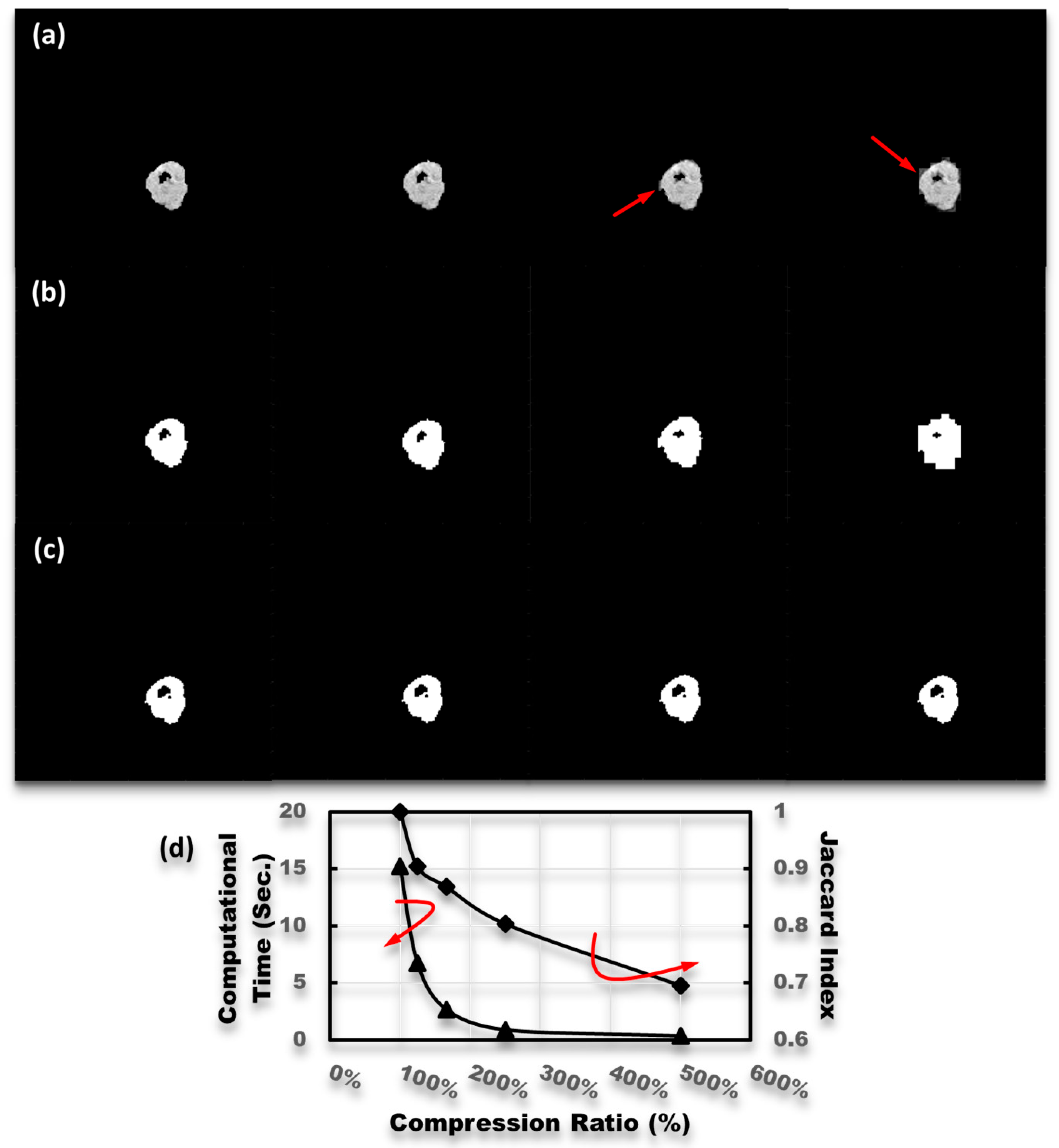
For estimating scores of the Jaccard index, the segmentation result illustrated in Figure 1(a3) was employed to be as a pseudo-ground truth. Then, four values of compression ratios, 125%, 167%, 250%, and 500%, were used to test the performance of the proposed method for tumor segmentation of tremendously small size medical images. The segmentation results with various compression ratios are sequentially shown in the first row of Figure 2. It should be emphasized that each segmentation image was reconstructed using a bicubic interpolation after corresponding image compression. The results, shown in Figure 2a, reveal the ability of the proposed method for automatically catching featured components from extreme small size medical images. However, the simplified reconstruction also caused some undesired consequences. As indicated by the red arrows shown in the last two columns of Figure 2a, some aliasing edges appeared. Those undesired aliasing edges significantly affected the scores of the Jaccard index. To estimate the scores of the Jaccard index and visually exhibit the consequences, the profiles of union and intersection areas between each reconstructed image and the pseudo-ground truth are, respectively, illustrated in Figure 2b,c. The curves of computational time and the Jaccard index are illustrated in Figure 2d. The illustration shows that, even when the compression ratio was set to be 500%, the score of the Jaccard index could have a nice value, about 0.7, while the computational time was only 0.3 s.

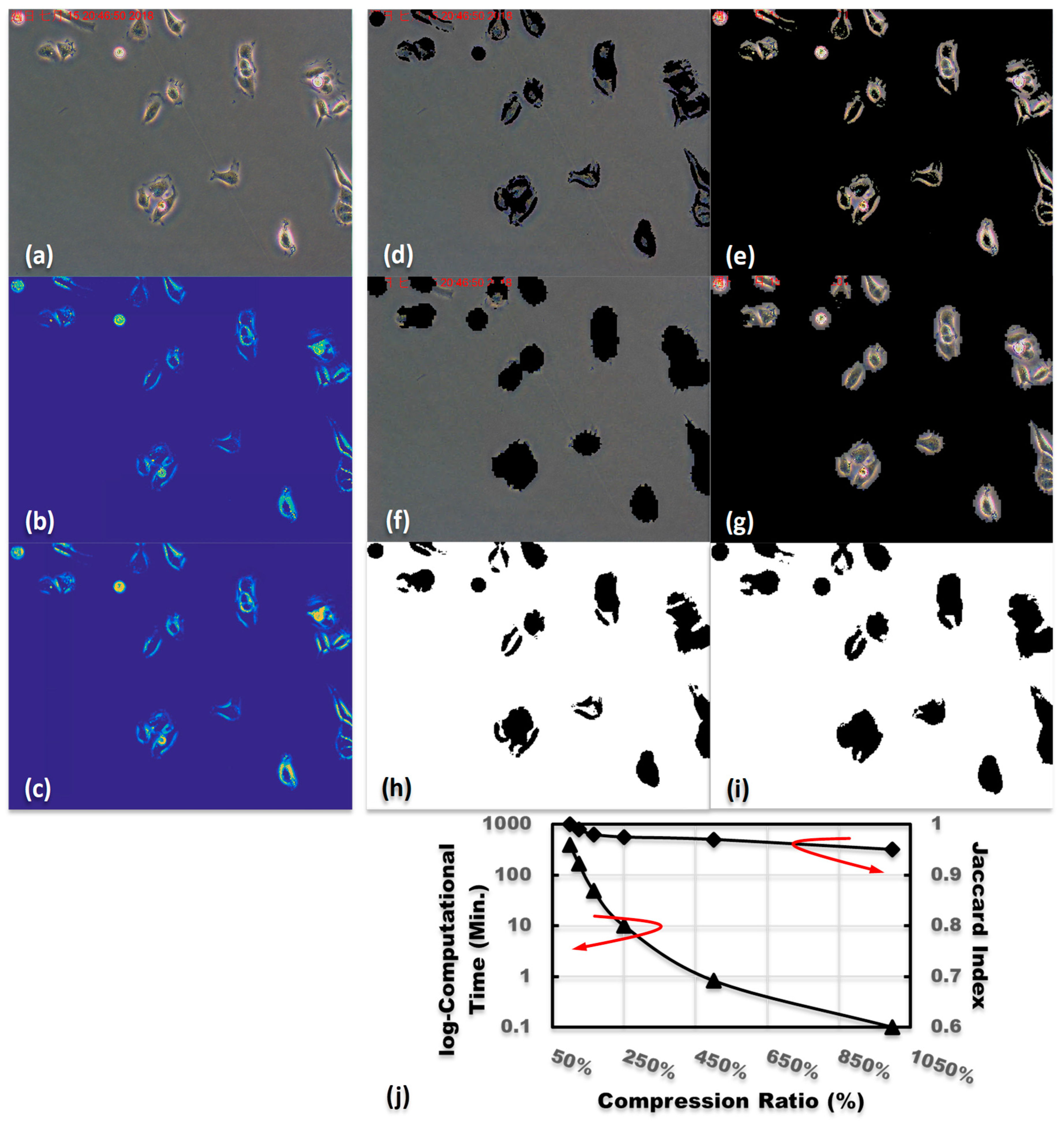
Furthermore, to test the performance of the proposed method in the image segmentation of tremendously large size medical images, a set of cell culturing images was utilized. The pixel sizes of the original cell culturing images are 1200 pixels by 1600 pixels. The pixel intensity in each case of the cell culturing image was first normalized to $\left[0,1\right]$, its global mean was subtracted, and the values lower than zero were set to be zero for preliminary denoising. Since the cells are specifically the only substance of foreground image, thus differing from the mentioned approach, the Yukawa potential kernel was assigned for measuring the specific local property. Figure 3 illustrates the segmentation results with and without dealing with the compression processes. The profiles of kinetic and potential energy density functionals of the original image, as shown in Figure 3a, are depicted in Figure 3b,c, respectively. As expected, the profile of the potential energy density functional was similar to that of the kinetic one. The reason is that the Yukawa potential is an extreme short potential; thus, it can significantly exhibit local properties of a physical particle of interest. The difference between the Yukawa potential energy density functional and the kinetic one is that the kinetic one has an extreme abrupt edge while the Yukawa one has a relatively alleviative edge due to the slight interaction adjacent to the boundaries. This means that the image boundaries can also be defined using the proposed Lagrangian density functional. In other words, the employed Yukawa potential kernel is suitable for measuring specific substance with strong localization. The segmented background and foreground are, respectively, shown in Figure 3d,e, while the corresponding compressed images with a 10-time compression ratio are, respectively, shown in Figure 3f,g. Then, the profiles of corresponding pixel areas of union and intersection are sequentially shown in Figure 3h,i. Figure 3j exhibits the curves of scores of the Jaccard index and log-computational time. As expected, the compressed results from the large size image had high scores of the Jaccard index as they still had enough featured components even after a 10-time image compression.

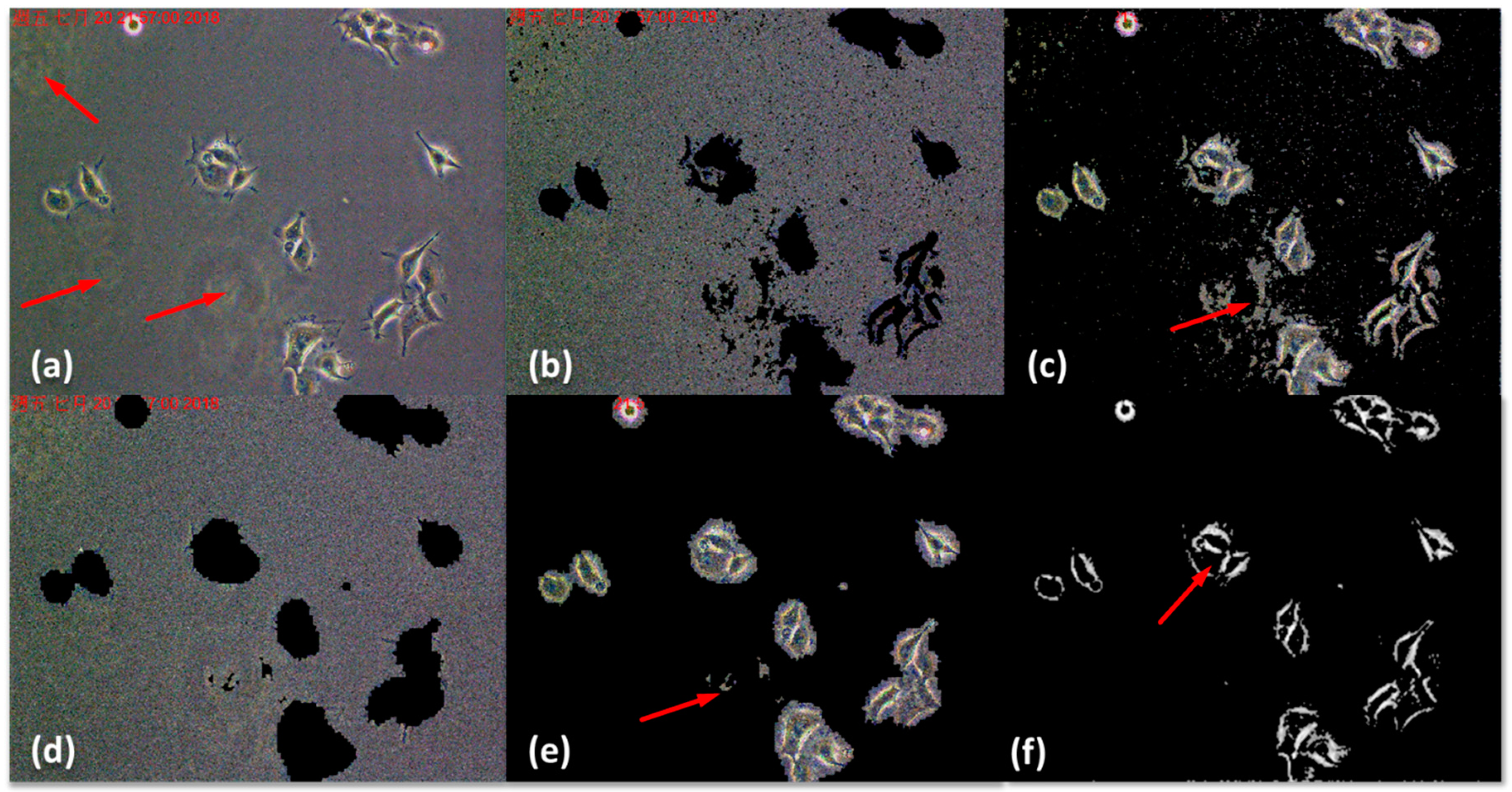
To test the performance of anti-noising of the proposed method, a cell-culturing image that has severe light and noise pollution was employed as an input image in the study. As illustrated in Figure 4a, the original size of the employed image is also 1200 pixels by 1600 pixels. Thus, computational times of this set should be similar to that of the image shown in Figure 3a. The noise was randomly distributed in the image, and the red arrows depicted the regions that have severe light pollution. The segmented background and foreground images of the original are illustrated in Figure 4b,c, respectively. As expected, the regions having severe pollution, such as indicated by the red arrow in Figure 4b, were also mapped back to the original image. The Yukawa potential kernel also enhanced the noise and the light spots. Then, several speckles caused by the noise also appeared in the foreground and background images. To inhibit the undesired featured components caused by the noise and the light pollution, the original image was compressed with a 10-time compression ratio and the segmentation results are illustrated in Figure 4d,e. Obviously, the noise and light pollution were sufficiently inhibited, thus the undesired featured components from those issues were filtered out by the global density functional estimations. The score of the Jaccard index of this reconstructed background image was 0.9178 and the computational time was about 5.7 s. To exhibit the comparison between the contemporary method and the proposed algorithm, a segmentation result by employing the Otsu’s method [63] is illustrated in Figure 4f. The Otsu’s method exhibited superior performance in time saving. It only costed 1.0 s to extract all of the borders of the cells. On other hand, it was also obvious that the method filtered out all information about intercellular substances inside each cell. It might cause an inconvenience on studying cell morphologies.

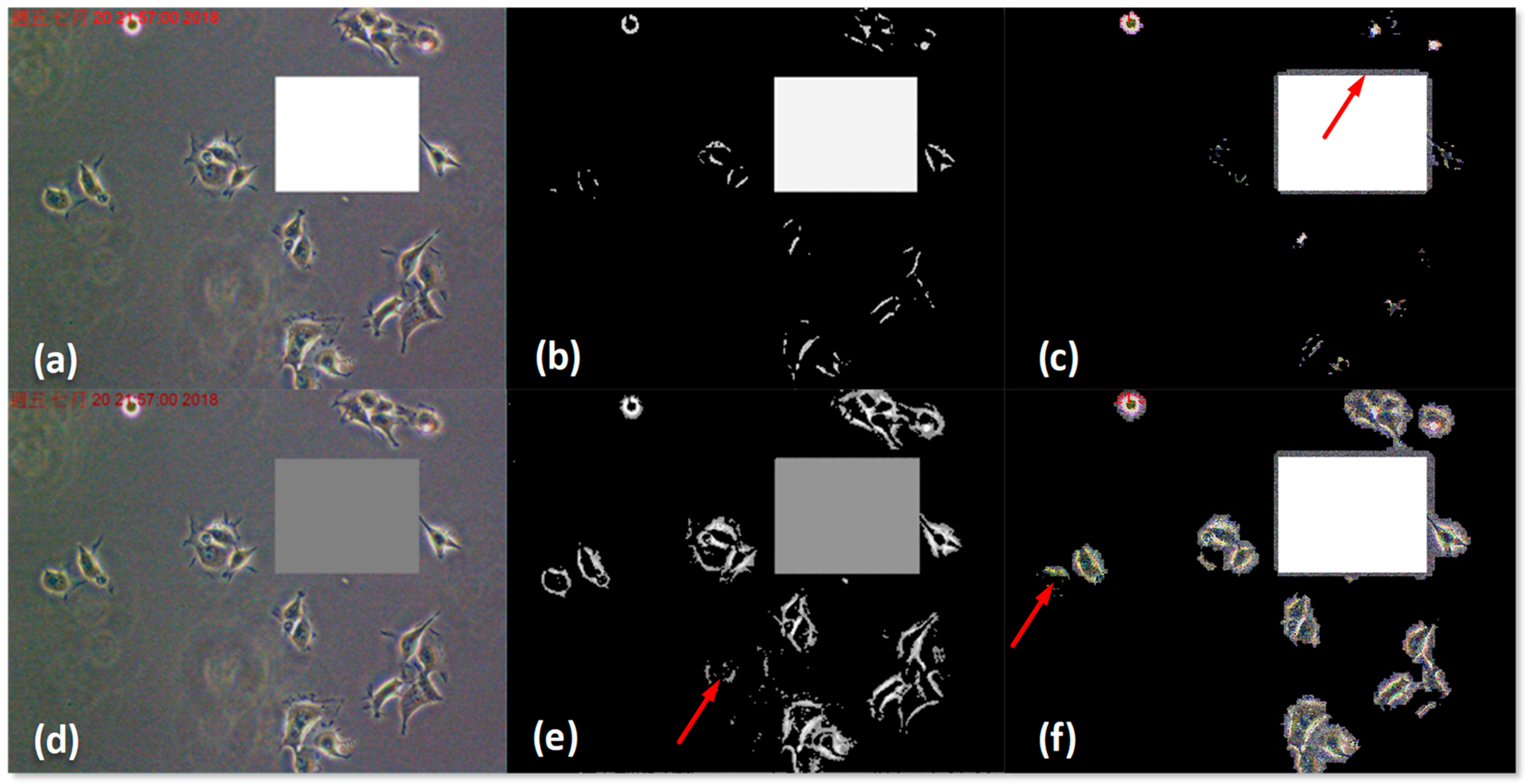
To search the limitation of the Otsu’s method and the proposed algorithm, a set of images with artifacts were also employed and the segmentation results are illustrated in Figure 5. Figure 5a,d exhibits the cell culturing images having artifacts with intensities of 1 and 0.5, respectively. Then, Figure 5b,c, respectively, shows the segmentation results by means of the Otsu’s method and the proposed algorithm in the case of Figure 5a. Similarly, Figure 5e,f shows the case of Figure 5d. In the case of Figure 5a, these two methods almost failed to extract the images of cell bodies from the original image. Meanwhile, a slight border extension of the artifact happens in Figure 5c, as indicated by the red arrow. By comparing the outcomes in Figure 4, the undesired components caused by the noise was extracted by the Otsu’s method, as indicated by the red arrow in Figure 5e. Then, an extended border of the artifact and a fragmented cell extracted by the proposed algorithm are illustrated in Figure 5f. Under the circumstance of employing the artifacts, the proposed algorithm could still extract the information of the intercellular substances inside each cell.

4. Discussion

Two different types of medical images were utilized to validate the proposed image segmentation method. The physical properties of the simple, square-root, and Yukawa potential kernels were investigated in detail to realize the diversity of reconstruction of the medical images in physical spaces. The square-root potential kernel exhibited a better smoothing performance than the simple one, whereas the Yukawa potential kernel focused on the local featured structures of the images. The experimental results reveal the feasibility of the proposed method for automatic medical image segmentation. Then, the images with various compression ratios were used to test the performance of the proposed method by extracting the featured components from both tremendously small and large imageries. As shown in Figure 2a, the compressed image with a 10-time compression ratio only had a size of 22 pixels by 22 pixels. The computational time and the score of the Jaccard index were, respectively, 0.3 s and 0.7. Thus, the segmentation result reveals that the proposed method could extract featured components from a tremendously small medical image. On the other hand, the proposed method provides an alternative for image denoising issues by reducing the image size, estimating the global density functionals, and then mapping back into the pixel space with original image sizes. The experimental result (Figure 4e) shows the successful inhibition of the noise and the light pollution compared to the image shown in Figure 4c. Furthermore, the limitations of the proposed algorithm are illustrated in Figure 5c,f.

5. Conclusions

Under the framework of data density functionals, the proposed method provides an avenue for medical image segmentation with adjustable computational complexity. It can automatically obtain the smoothened segmentation results by introducing the square-root potential kernel. Meanwhile, by utilizing the Yukawa potential kernel, the foreground and the background of a medical image can be easily segmented. Furthermore, the technique can also be used to inhibit the noise and the light pollution that occur in medical images.

References

- Senft, C.; Bink, A.; Franz, K.; Vatter, H.; Gasser, T.; Seifert, V. Intraoperative MRI guidance and extent of resection in glioma surgery: A randomised, controlled trial. Oncology 2011, 12, 997–1003. [Google Scholar] [CrossRef]
- Bullock, P.; Dunaway, D.; McGurk, L.; Richards, R. Integration of image guidance and rapid prototyping technology in craniofacial surgery. Int. J. Oral Maxillofac. Surg. 2013, 42, 970–973. [Google Scholar] [CrossRef] [PubMed]
- Kenngott, H.G.; Wagner, M.; Gondan, M.; Nickel, F.; Nolden, M.; Fetzer, A.; Weitz, J.; Fischer, L.; Speidel, S.; Meinzer, H.-P.; et al. Real-time image guidance in laparoscopic liver surgery: First clinical experience with a guidance system based on intraoperative CT imaging. Surg. Endosc. 2014, 28, 933–940. [Google Scholar] [CrossRef] [PubMed]
- Nowitzke, A.; Wood, M.; Cooney, K. Improving accuracy and reducing errors in spinal surgery—A new technique for thoracolumbar-level localization using computer-assisted image guidance. Spine J. 2008, 8, 597–604. [Google Scholar] [CrossRef] [PubMed]
- Smistad, E.; Falch, T.L.; Bozorgi, M.; Elster, A.C.; Lindseth, F. Medical image segmentation on GPUs—A comprehensive review. Med. Image Anal. 2015, 20, 1–18. [Google Scholar] [CrossRef] [PubMed]
- Zhu, J.; Liu, A.-A.; Chen, M.; Tasdizen, T.; Su, H. Special Issue on Biomedical Big Data: Understanding, Learning and Applications. IEEE Trans. Big Data 2017, 3, 375–377. [Google Scholar] [CrossRef]
- Hsieh, J.; Nett, B.; Yu, Z.; Sauer, K.; Thibault, J.-B.; Bouman, C.A. Recent Advances in CT Image Reconstruction. Curr. Radiol. Rep. 2013, 1, 39–51. [Google Scholar] [CrossRef] [Green Version]
- Kim, J.; Duchin, Y.; Shamir, R.R.; Patriat, R.; Vitek, J.; Harel, N.; Sapiro, G. Automatic localization of the subthmlamic nucleus on patient-specific clinical by incorporating 7 T MRI and machine learning: Application in deep brain stimulation. Hum. Brain Mapp. 2018, 40, 679–698. [Google Scholar] [CrossRef]
- Bauer, S.; Wiest, R.; Nolte, L.P.; Reyes, M. A survey of MRI-based medical image analysis for brain tumor studies. Phys. Med. Biol. 2013, 58, R97–R129. [Google Scholar] [CrossRef] [PubMed]
- Norouzi, A.; Rahim, M.S.M.; Altameem, A.; Saba, T.; Rad, A.E.; Rehman, A.; Uddin, M. Medical Image Segmentation Methods, Algorithms, and Applications. IETE Tech. Rev. 2014, 31, 199–213. [Google Scholar] [CrossRef]
- Huang, S.-J.; Wu, C.-J.; Chen, C.-C. Pattern Recognition of Human Postures Using Data Density Functional Method. Appl. Sci. 2018, 8, 1615. [Google Scholar] [CrossRef]
- Wu, C.-J.; Huang, S.-J.; Chen, C.-C. Method on Pattern Recognition of Various Limb Postures. J. Biomed. Syst. Emerg. Technol. 2018, 5, 118. [Google Scholar]
- Přibil, J.; Přibilová, A.; Frollo, I. Two Methods of Automatic Evaluation of Speech Signal Enhancement Recorded in the Open-Air MRI Environment. Meas. Sci. Rev. 2017, 17, 257–263. [Google Scholar] [CrossRef] [Green Version]
- Glasser, M.F.; Smith, S.M.; Marcus, D.S.; Andersson, J.L.; Auerbach, E.J.; Behrens, T.E.; Coalson, T.S.; Harms, M.P.; Jenkinson, M.; Moeller, S.; et al. The Human Connectome Project’s neuroimaging approach. Nat. Neurosci. 2016, 19, 1175–1187. [Google Scholar] [CrossRef]
- Bas, E.; Erdogmus, D.; Draft, R.W.; Lichtman, J.W. Local tracing of curvilinear structures in volumetric color images: Application to the Brainbow analysis. J. Vis. Commun. Image R 2012, 23, 1260–1271. [Google Scholar] [CrossRef]
- Liu, Q.; Wang, S.; Yang, K.; Luo, J.; Zhu, Y.M.; Liang, D. Highly Undersampled Magnetic Resonance Image Reconstruction Using Two-Level Bregman Method with Dictionary Updating. IEEE Trans. Med. Imaging 2013, 32, 1290–1301. [Google Scholar] [CrossRef] [PubMed]
- Qu, X.; Hou, Y.; Lam, F.; Guo, D.; Zhong, J.; Chen, Z. Magnetic resonance image reconstruction from undersampled measurements using a patch-based nonlocal operator. Med. Image Anal. 2014, 18, 843–856. [Google Scholar] [CrossRef]
- Trémoulhéac, B.; Dikaios, N.; Atkinson, D.; Arridge, S.R. Dynamic MR Image Reconstruction-Separation From Undersampled (k,t)-Space via Low-Rank Plus Sparse Prior. IEEE Trans. Med. Imaging 2014, 33, 1689–1701. [Google Scholar] [CrossRef]
- Wang, S.; Zhang, Y.; Liu, G.; Phillips, P.; Yuan, T.F. Detection of Alzheimer’s Disease by Three-Dimensional Displacement Field Estimation in Structural Magnetic Resonance Imaging. J. Alzheimers Dis. 2016, 50, 233–248. [Google Scholar] [CrossRef]
- Zhang, Y.; Wang, S.; Phillips, P.; Yang, J.; Yuan, T.F. Three-Dimensional Eigenbrain for the Detection of Subjects and Brain Regions Related with Alzheimer’s Disease. J. Alzheimers Dis. 2016, 50, 1163–1179. [Google Scholar] [CrossRef]
- Dormont, D.; Seidenwurm, D.; Galanaud, D.; Cornu, P.; Yelnik, J.; Bardinet, E. Neuroimaging and deep brain stimulation. AJNR Am. J. Neuroradiol. 2010, 31, 15–23. [Google Scholar] [CrossRef]
- Volkmann, J. Update on surgery for Parkinson’s disease. Curr. Opin. Neurol. 2007, 20, 465–469. [Google Scholar] [CrossRef]
- Abosch, A.; Yacoub, E.; Ugurbil, K.; Harel, N. An assessment of current brain targets for deep brain stimulation surgery with susceptibility-weighted imaging as 7 tesla. Neurosurgery. 2010, 67, 1745–1756. [Google Scholar] [CrossRef]
- Lefranc, M.; Derrey, S.; Merle, P.; Tir, M.; Constans, J.M.; Montpellier, D.; Macron, J.M.; Le Gars, D.; Peltier, J.; Baledentt, O.; et al. High-Resolution 3-Dimensional T2*-Weighted Angiography (HR 3-D SWAN): An Optimized 3-T Magnetic Resonance Imaging Sequence for Targeting the Subthalamic Nucleus. Neurosurgery 2014, 74, 615–626. [Google Scholar] [CrossRef]
- Zonenshayn, M.; Rezai, A.R.; Mogilner, A.Y.; Beric, A.; Sterio, D.; Kelly, P.J. Comparison of Anatomic and Neurophysiological Methods for Subthalamic Nucleus Targeting. Neurosurgery 2000, 47, 282–292. [Google Scholar] [CrossRef]
- Vertinsky, A.T.; Coenen, V.A.; Lang, D.J.; Kolind, S.; Honey, C.R.; Li, D.; Rauscher, A. “Localization of the Subthalamic Nucleus: Optimization with Susceptibility-Weighted Phase MR Imaging. AJNR Am. J. Neuroradiol. 2009, 30, 1717–1724. [Google Scholar] [CrossRef]
- Schäfer, A.; Forstmann, B.U.; Neumann, J.; Wharton, S.; Mietke, A.; Bowtell, R.; Turner, R. “Direct visualization of the subthalamic nucleus and its iron distribution using high-resolution susceptibility mapping. Hum. Brain Mapp. 2012, 33, 2831–2842. [Google Scholar] [CrossRef]
- Manova, E.S.; Habib, C.A.; Boikov, A.S.; Ayaz, M.; Khan, A.; Kirsch, W.M.; Kido, D.K.; Haacke, E.M. Characterizing the Mesencephalon Using Susceptibility-Weighted Imaging. AJNR Am. J. Neuroradiol. 2009, 30, 569–574. [Google Scholar] [CrossRef]
- Bastos Leite, A.J.; van Straaten, E.C.; Scheltens, P.; Lycklama, G.; Barkhof, F. Thalamic Lesions in Vascular Dementia: Low Sensitivity of Fluid-Attenuated Inversion Recovery (FLAIR) Imaging. Stroke 2004, 35, 415–419. [Google Scholar] [CrossRef]
- Olindo, S.; Chausson, N.; Joux, J.; Saint-Vil, M.; Signate, A.; Edimonana-Kapute, M.; Jeannine, S.; Mejdoubi, M.; Aveillan, M.; Cabre, P.; et al. Fluid-Attenuated Inversion Recovery Vascular Hyperintensity: An Early Predictor of Clinical Outcome in Proximal Middle Cerebral Artery Occlusion. Arch. Neurol. 2012, 69, 1462–1468. [Google Scholar] [CrossRef]
- Essig, M.; Knopp, M.V.; Schoenberg, S.O.; Hawighorst, H.; Wenz, F.; Debus, J.; van Kaick, G. Cerebral Gliomas and Metastases: Assessment with Contrast-enhanced Fast Fluid-attenuated Inversion-Recovery MR Imaging. Radiology 1999, 210, 551–557. [Google Scholar] [CrossRef] [PubMed]
- Chen, C.-C.; Juan, H.-H.; Tsai, M.-Y.; Lu, H.H.-S. Unsupervised Learning and Pattern Recognition of Biological Data Structures with Density Functional Theory and Machine Learning. Sci. Rep. 2018, 8, 557. [Google Scholar] [CrossRef] [PubMed] [Green Version]
- Taubman, D. High Performance Scalable Image Compression with EBCOT. IEEE Trans. Image Process. 2000, 9, 1158–1170. [Google Scholar] [CrossRef] [PubMed]
- Shapiro, J.M. An embedded hierarchical image coder using zerotrees of wavelet coefficients. In Proceedings of the IEEE Data Compression Conference, Snowbird, UT, USA, 30 March–2 April 1993; pp. 214–223. [Google Scholar]
- Said, A.; Pearlman, W. A new, fast and efficient image codec based on set partitioning in hierarchical trees. IEEE Trans. Circuits Syst. Video Technol. 1996, 6, 243–250. [Google Scholar] [CrossRef]
- Taubman, D.; Zakhor, A. Multi-rate 3-D subband coding of video. IEEE Trans. Image Process. 1994, 3, 572–588. [Google Scholar] [CrossRef]
- Mallat, S.G. A theory for multiresolution signal decomposition: The wavelet representation. IEEE Trans. Pattern Anal. Mach. Intell. 1989, 11, 674–693. [Google Scholar] [CrossRef]
- Toderici, G.; Vincent, D.; Johnston, N.; Hwang, S.J.; Minnen, D.; Shor, J.; Covell, M. Full Resolution Image Compression with Recurrent Neural Networks. In Proceedings of the IEEE Conference on Computer Vision and Pattern Recognition, Honolulu, Hawaii, 21–26 July 2017. [Google Scholar]
- Toderici, G.; O’Malley, S.M.; Hwang, S.J.; Vincent, D.; Minnen, D.; Baluja, S.; Covell, M.; Sukthankar, R. Variable Rate Image Compression with Recurrent Neural Networks. arXiv 2016, arXiv:1511.06085. [Google Scholar]
- Theis, L.; Shi, W.; Cunningham, A.; Huszár, F. Lossy Image Compression with Compressive Autoencoders. arXiv 2017, arXiv:1703.00395v1. [Google Scholar]
- Kim, U.S.; Sunwoo, M.H. New Frame Rate Up-Conversion Algorithms with Low Computational Complexity. IEEE Trans. Circ. Syst. Vid. 2014, 24, 384–393. [Google Scholar] [CrossRef]
- Jiang, F.; Tao, W.; Liu, S.; Ren, J.; Guo, X.; Zhao, D. An End-to-End Compression Framework Based on Convolutional Neural Networks. IEEE Trans. Circ. Syst. Vid. 2018, 28, 3007–3018. [Google Scholar] [CrossRef] [Green Version]
- Liu, H.; Chen, T.; Shen, Q.; Yue, T.; Ma, Z. Deep Image Compression via End-to-End Learning. arXiv 2018, arXiv:1806.01496v1. [Google Scholar]
- Han, S.; Mao, H.; Dally, W.J. Deep Compression: Compressing Deep Neural Networks with Pruning, Trained Quantization and Huffman Coding. arXiv 2016, arXiv:1510.00149v5. [Google Scholar]
- Krizhevsky, A.; Sutskever, I.; Hinton, G.E. ImageNet classification with deep convolutional neural networks. In Proceedings of the 25th International Conference on Neural Information Processing Systems, Lake Tahoe, NV, USA, 3–6 December 2012. [Google Scholar]
- Zhang, X.; Zhou, X.; Lin, M.; Sun, J. ShuffleNet: An Extremely Efficient Convolutional Neural Network for Mobile Devices. arXiv 2017, arXiv:1707.01083v2. [Google Scholar]
- Han, S.; Liu, X.; Mao, H.; Pu, J.; Pedram, A.; Horowitz, M.A.; Dally, W.J. EIE: Efficient Inference Engine on Compressed Deep Neural Network. arXiv 2016, arXiv:1602.01528v2. [Google Scholar] [CrossRef]
- Pratondo, A.; Chui, C.-K.; Ong, S.-H. Robust Edge-Stop Functions for Edge-Based Active Contour Models in Medical Image Segmentation. IEEE Signal Proc. Lett. 2016, 23, 222–226. [Google Scholar] [CrossRef]
- Chen, L.-C.; Papandreou, G.; Kokkinos, I.; Murphy, K.; Yuille, A.L. DeepLab: Semantic Image Segmentation with Deep Convolutional Nets, Atrous Convolution, and Fully Connected CRFs. IEEE Trans. Pattern Anal. Mach. Intell. 2018, 40, 834–848. [Google Scholar] [CrossRef] [Green Version]
- Milletari, F.; Navab, N.; Ahmadi, S.-A. V-Net: Fully Conventional Neural Networks for Volumetric Medical Image Segmentation. In Proceedings of the 4th International Conference on 3D Vision, Stanford, CA, USA, 25–28 October 2016. [Google Scholar]
- Zhang, W.; Li, R.; Deng, H.; Wang, L.; Lin, W.; Ji, S.; Shen, D. Deep convolutional neural networks for multi-modality isointense infant brain image segmentation. Neuroimage 2015, 108, 214–224. [Google Scholar] [CrossRef]
- Hsu, Y.; Lu, H.H.-S. Brainbow image segmentation using Bayesian sequential partitioning. Int. J. Comput. Inf. Syst. Control Eng. 2013, 7, 891–896. [Google Scholar]
- Wu, T.-Y.; Juan, H.-H.; Lu, H.H.-S.; Chiang, A.-S. A crosstalk tolerated neural segmentation methodology for brainbow images. In Proceedings of the International Symposium on Applied Sciences in Biomedical and Communication Technologies (ACM ISABEL), Barcelona, Spain, 26–29 October 2011. [Google Scholar]
- Morar, A.; Moldoveanu, F.; Gröller, E. Image Segmentation Based on Active Contours without Edges. In Proceedings of the IEEE 8th International Conference on Intelligent Computer Communication and Processing, Cluj-Napoca, Romania, 30 August–1 September 2012. [Google Scholar]
- Kass, M.; Witkin, A.; Terzopoulos, D. Snakes: Active contour models. Int. J. Comput. Vision. 1988, 1, 321–331. [Google Scholar] [CrossRef] [Green Version]
- Arbeláez, P.; Maire, M.; Fowlkes, C.; Malik, J. Contour Detection and Hierarchical Image Segmentation. IEEE Trans. Pattern Anal. Mach. Intell. 2011, 33, 898–916. [Google Scholar] [CrossRef] [Green Version]
- Mandal, D.; Chatterjee, A.; Maitra, M. Robust medical image segmentation using particle swarm optimization aided level set based global fitting energy active contour approach. Eng. Appl. Artif. Intell. 2014, 35, 199–214. [Google Scholar] [CrossRef]
- Wang, L.; Pan, C. Robust level set image segmentation via a local correntropy-based k-means clustering. Pattern Recognit. 2014, 47, 1917–1925. [Google Scholar] [CrossRef]
- Li, C.; Huang, R.; Ding, Z.; Gatenby, J.C.; Metaxas, D.N.; Gore, J.C. A Level Set Method for Image Segmentation in the Presence of Intensity Inhomogeneities with Application to MRI. IEEE Trans. Image Process. 2011, 20, 2007–2016. [Google Scholar] [CrossRef] [PubMed]
- Li, C.; Xu, C.; Gui, C.; Fox, M.D. Distance Regularization Level Set Evolution and Its Application to Image Segmentation. IEEE Trans. Image Process. 2010, 19, 3243–3254. [Google Scholar] [CrossRef] [PubMed]
- Rowlinson, J.S. The Yukawa potential. Phys. A Stat. Mech. Appl. 1989, 156, 15–34. [Google Scholar] [CrossRef]
- Moon, N.; Bullitt, E.; van Leemput, K.; Gerig, G. Automatic brain and tumor segmentation. In Proceedings of the 5th International Conference on Medical Image Computing and Computer-Assisted Intervention, Tokyo, Japan, 25–28 September 2002. [Google Scholar]
- Cai, H.; Yang, Z.; Cao, X.; Xia, W.; Xu, X. A New Iterative Triclass Thresholding Technique in Image Segmentation. IEEE Trans. Image Process. 2014, 23, 1038–1046. [Google Scholar] [CrossRef]
Figure 1.
Two original MR images, as shown in (a1,b1), sourced from Ref. [62] were employed to study performances of those utilized potential kernels. Regions of interest in each MR image were defined to avoid undesired segmentation results from skulls by red rectangular windows. According to the estimated morphologies of energy density functionals, shown in the late two columns, the segmentation results were obtained using the proposed framework and are as illustrated in second and third columns, as respectively shown from (a2) to (a5) and from (b2) to (b5). It is noted that the potential kernel used in (a7) and (b7) was the simple potential kernel, while that used in (a8) and (b8) was the square-root potential kernel.
Figure 2.
The segmentation results with the compression rate of 125%, 167%, 250%, and 500% are respectively shown in (a) row. Then, all of them were reconstructed using the bicubic interpolation. It is obvious that aliasing edges also appeared, as indicated by the red arrows in (a) row, after the strong image compression. The (b,c) rows, respectively, illustrated the union and the intersection areas between the testing images and the ground truth. (d) The curves of computational times and scores of the Jaccard index with various compression ratios.
Figure 3.
The profile of the employed cell culturing image (a), and the corresponding profiles of kinetic and potential energy density functionals, respectively (b,c). The background and foreground images of (a), respectively (d,e). The images after a 10-time compression, respectively (f,g). The areas of pixel union and the intersection between (e,g), respectively (h,i). (j) The curves of log-computational times and the scores of the Jaccard index for the cases of various compression ratios.
Figure 4.
(a) A cell culturing image with severe noise and light pollution. The red arrows were used to indicate the locations of pollution. (b,c) The segmented background and foreground, respectively. The undesired pollution was still extracted by the proposed method, as indicated by the red arrow. (d,e) By further increasing the compression ratio, the reconstructed background and foreground had a significant improvement. (f) The segmentation result by employing the Otsu’s method [63]. It is worth noting that the important information regarding the intercellular substance was filtered out by the Otsu’s method.
Figure 5.
The comparison of cell segmentation between the Otsu’s method and the proposed algorithm. Two artifacts with different intensities were added into the original image from Figure 4a to study the performances of these two methods. The intensity of the artifact in (a) is 1, while that in (d) is 0.5. The segmentation results (b,c) show the limitations of the methods. Then, the results (e,f) show the acceptable profiles of cell image segmentation compared to those in Figure 4e,f, respectively. The important information regarding the intercellular substances inside each cell were also extracted by the proposed algorithm (f).
© 2019 by the authors. Licensee MDPI, Basel, Switzerland. This article is an open access article distributed under the terms and conditions of the Creative Commons Attribution (CC BY) license (http://creativecommons.org/licenses/by/4.0/).
Share and Cite
MDPI and ACS Style
Chen, C.-C.; Tsai, M.-Y.; Kao, M.-Z.; Lu, H.H.-S. Medical Image Segmentation with Adjustable Computational Complexity Using Data Density Functionals. Appl. Sci. 2019, 9, 1718. https://0-doi-org.brum.beds.ac.uk/10.3390/app9081718
AMA Style
Chen C-C, Tsai M-Y, Kao M-Z, Lu HH-S. Medical Image Segmentation with Adjustable Computational Complexity Using Data Density Functionals. Applied Sciences. 2019; 9(8):1718. https://0-doi-org.brum.beds.ac.uk/10.3390/app9081718
Chicago/Turabian StyleChen, Chien-Chang, Meng-Yuan Tsai, Ming-Ze Kao, and Henry Horng-Shing Lu. 2019. "Medical Image Segmentation with Adjustable Computational Complexity Using Data Density Functionals" Applied Sciences 9, no. 8: 1718. https://0-doi-org.brum.beds.ac.uk/10.3390/app9081718
Note that from the first issue of 2016, this journal uses article numbers instead of page numbers. See further details here.