Path Loss Prediction Based on Machine Learning: Principle, Method, and Data Expansion


1
School of Information and Electronics, Beijing Institute of Technology, Beijing 100081, China
2
Department of Electronic Engineering, Tsinghua University, Beijing 100084, China
*
Author to whom correspondence should be addressed.
Appl. Sci. 2019, 9(9), 1908; https://0-doi-org.brum.beds.ac.uk/10.3390/app9091908
Submission received: 1 April 2019
/
Revised: 28 April 2019
/
Accepted: 3 May 2019
/
Published: 9 May 2019
(This article belongs to the Section Electrical, Electronics and Communications Engineering)
Abstract
:Path loss prediction is of great significance for the performance optimization of wireless networks. With the development and deployment of the fifth-generation (5G) mobile communication systems, new path loss prediction methods with high accuracy and low complexity should be proposed. In this paper, the principle and procedure of machine-learning-based path loss prediction are presented. Measured data are used to evaluate the performance of different models such as artificial neural network, support vector regression, and random forest. It is shown that these machine-learning-based models outperform the log-distance model. In view of the fact that the volume of measured data sometimes cannot meet the requirements of machine learning algorithms, we propose two mechanisms to expand the training dataset. On one hand, old measured data can be reused in new scenarios or at different frequencies. On the other hand, the classical model can also be utilized to generate a number of training samples based on the prior information obtained from measured results. Measured data are employed to verify the feasibility of these data expansion mechanisms. Finally, some issues for future research are discussed.
1. Introduction
Radio wave propagation plays an important role in the research and development of wireless communication systems. The wireless signal strength decreases as the distance between the transmitter and receiver increases. Moreover, the mechanisms of the electromagnetic wave propagation are diverse and can be generally classified as reflection, diffraction, and scattering [1]. The complex propagation environment makes the prediction of the received signal strength a very hard problem.
Path loss is used to describe the attenuation of an electromagnetic wave as it propagates through space [2]. An accurate, simple, and general model for the path loss is essential for link budget, coverage prediction, system performance optimization, and selection of base station (BS) locations. Consequently, researchers and engineers have made great efforts to find out reasonable models for the path loss prediction in different scenarios and at different frequencies. Many measurement campaigns have been conducted worldwide to collect data, which have been used to build, adjust, and evaluate these models.
The upcoming fifth-generation (5G) networks are designed to support increased throughput, wide coverage, improved connection density, reduced radio latency, and enhanced spectral efficiency. Supporting Internet of Things (IoT) applications will involve vast coverage areas and various terrains. Besides, new frequency bands like the sub-6 GHz and millimeter wave bands, will be exploited to provide wide bandwidths. Numerous measurement campaigns and drive tests have to be carried out to collect attenuation data at the new frequencies. The network planning of 5G mobile communication systems will confront severe challenges, and preferable models are required for the path loss prediction.
Traditionally, path loss prediction models have been built based on empirical or deterministic methods [3]. Empirical models mainly rely on measurements in a given frequency range and a specific scenario. They provide statistical descriptions of the relationship between path loss and propagation parameters such as frequency, antenna-separation distance, antenna heights, and so on. For example, the log-distance model [4] uses the path loss exponent, which is determined empirically, to characterize how the receiver power falls off with the antenna-separation distance. A Gaussian random variable with zero mean is used to depict the attenuation (in decibel) caused by the shadow fading. Other typical empirical models include the Bullington, Egli, Longley-Rice, Okumura, and Hata models [2]. Empirical models are quite simple because few parameters are required and model equations are concise. However, parameters of empirical models are extracted from measured data in a specific scenario. Thus, their accuracy may be unsatisfactory when these models are applied to more general environments [5]. At the same time, empirical models can only represent the statistics of the path loss at a given distance, but they cannot give the actual received power at a specific location.
Deterministic models, such as models based on ray tracing and finite-difference time-domain (FDTD), apply radio-wave propagation mechanisms and numerical analysis techniques for modeling computational electromagnetics. In general, they can achieve high accuracy and provide the path loss value at any specific position. However, their disadvantages include the lack of computational efficiency and therefore prohibitive computation time in real environments. Site-specific geometry information and dielectric properties of materials are also required. Moreover, we have to run the time-consuming computation procedure again once the propagation environment has changed.
Machine learning is a method based on an extensive dataset and a flexible model architecture to make predictions. Recently, machine-learning-based methods have been used in self-driving cars, data mining, computer vision, speech recognition, and many other fields. These tasks can be classified as supervised learning and unsupervised learning. With labeled data, the goal of supervised learning is to learn a general and accurate function between inputs and outputs, which makes it suitable for solving classification and regression problems. On the other hand, unsupervised learning algorithms have to describe the hidden structure from unlabeled data. In essence, path loss prediction is a supervised regression problem, so it can also be solved by supervised machine learning algorithms, such as artificial neural network (ANN), support vector regression (SVR), and decision tree. It has been reported that the machine-learning-based models are more accurate than empirical models and more computational efficient than deterministic ones [3,6].
Among these machine-learning-based models, ANN, especially back propagation neural network (BPNN), has been widely used for path loss prediction. In [3], ANNs with different hidden neurons and different training algorithms were analyzed based on measured data collected in a rural environment. It was indicated that more complex ANNs do not considerably increase the prediction accuracy. In [7], a path loss prediction model based on BPNN was proposed for railway environment and it had good prediction accuracy and generalization ability for similar scenarios. In [8], a pure ANN system and a hybrid prediction system were designed for urban and suburban environments. It was illustrated that the ANN modeling approach provided more accurate prediction of field strength loss than that of COST231-Walfisch-Ikegami model. In [5], an ANN-based model was designed to predict the path loss values for heterogeneous networks, in which several frequencies and different environments including urban, suburban, and rural scenarios are considered. Compared with empirical models, the results showed that ANN performed well in terms of precision but with a slight increase of processing time and memory consumption. For indoor environments, a multilayer perceptron and a generalized regression neural network were proposed in [9] at the frequency of 1890 MHz, which showed a good agreement with the measurements. A propagation model using BPNN was developed within multi-wall and multi-frequency scenarios in [10]. In [11], parameters related to body shadowing and furniture effects were added to inputs and the proposed ANN model demonstrated high performance compared to empirical model and measurements. Besides BPNN, radial basis function neural network (RBF-NN) [12], dynamic neural networks (DNN) [13], and wavelet neural network [14], were also employed for path loss prediction. Recently, Neuro-Fuzzy draw great interests in the path loss prediction because of its transparency [15,16].
SVR was used for the prediction of radio-wave path loss values in suburban environments in [17,18]. Some algorithms, including genetic algorithms (GA) and tabu search (TS), were applied to select important parameters for SVR-based predictors. In [19], a SVR-based modeling method was presented to predict in-cabin path loss values at 3520 MHz, outperforming the curve fitting model. In [20], a propagation loss prediction model was built on the basis of SVR and it was able to achieve a good accuracy at the price of an acceptable computational cost.
Other machine learning algorithms such as decision tree and K-Nearest-Neighbors (KNN) were also employed for path loss prediction. In [21], random forest (RF) and KNN are exploited to predict the path loss in an urban environment for UAV communications. Results have shown that machine-learning-based models have high prediction accuracy and acceptable computational efficiency. Besides, feature importance is assessed by using RF algorithm. In [22], a hybrid scheme based on the ray tracing method and RF was presented for the field strength prediction. In contrast with the results of the finite integral method, the proposed model achieved higher prediction accuracy with less computation time. In [23], the received signal strengths were predicted for an environmental wireless sensor network by using several candidate machine learning algorithms, including Adaboost, RF, ANN, and KNN. Among these methods, RF showed the highest accuracy in the considered environment, achieving a significant reduction in the average prediction error compared to the empirical models. From the perspective of feature reduction, the authors used a variety of manifold learning methods to reduce the original feature dimension to two dimensions to establish a path loss model in [24].
The diverse application scenarios in the 5G era pose a great challenge to the channel models. A flexible modeling framework should be built to satisfy the requirements for the applications at new frequencies and in new propagation environments. As mentioned above, machine-learning-based methods are able to provide a tradeoff between accuracy and complexity of the path loss models. Nevertheless, machine learning is a data-hungry technique whose performance heavily depends on the amount and quality of the training data. Due to the high cost of conducting measurements, the path loss dataset is always far from the concept of “big data” which can be easily obtained on the Internet or Internet of Things (IoT). Especially when new scenarios or new frequencies are put into use, it is difficult to collect enough data for the path loss prediction in a short time. Therefore, data expansion solutions are also proposed in this paper to fill the research gap.
The major contributions of this paper can be summarized as follows.
- (1)
- The basic principle and procedure of the path loss prediction based on machine learning are presented. Some crucial issues such as data collection, data preprocessing, algorithm selection, model hyperparameter settings, and performance evaluation, are discussed.
- (2)
- In order to obtain enough data for machine-learning-based models, two mechanisms are proposed to enlarge the training dataset by taking full advantage of the existing data and the classical models. Data transferring is considered in both the scenario dimension and the frequency dimension.
- (3)
- Different machine learning algorithms are employed to validate the proposed methods based on the measured data. Both outdoor and indoor scenarios are taken into account and measured data are used to verify the feasibility of the machine-learning-based predictors.
The remainder of this paper is structured as follows. The procedure of machine-learning-based path loss prediction is presented in Section 2. Section 3 introduces some representative machine learning methods for regression task, including ANN, SVR, and decision tree. In Section 4, data expansion solutions are proposed and verified with the measured data in an outdoor urban scenario and an indoor aircraft cabin scenario. In Section 5, some issues for future path loss prediction based on machine learning methods are discussed. At last, conclusions are drawn in Section 6.
2. Machine-Learning-Based Path Loss Prediction
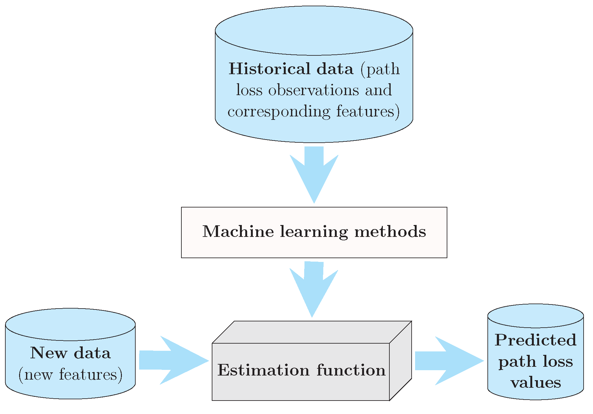
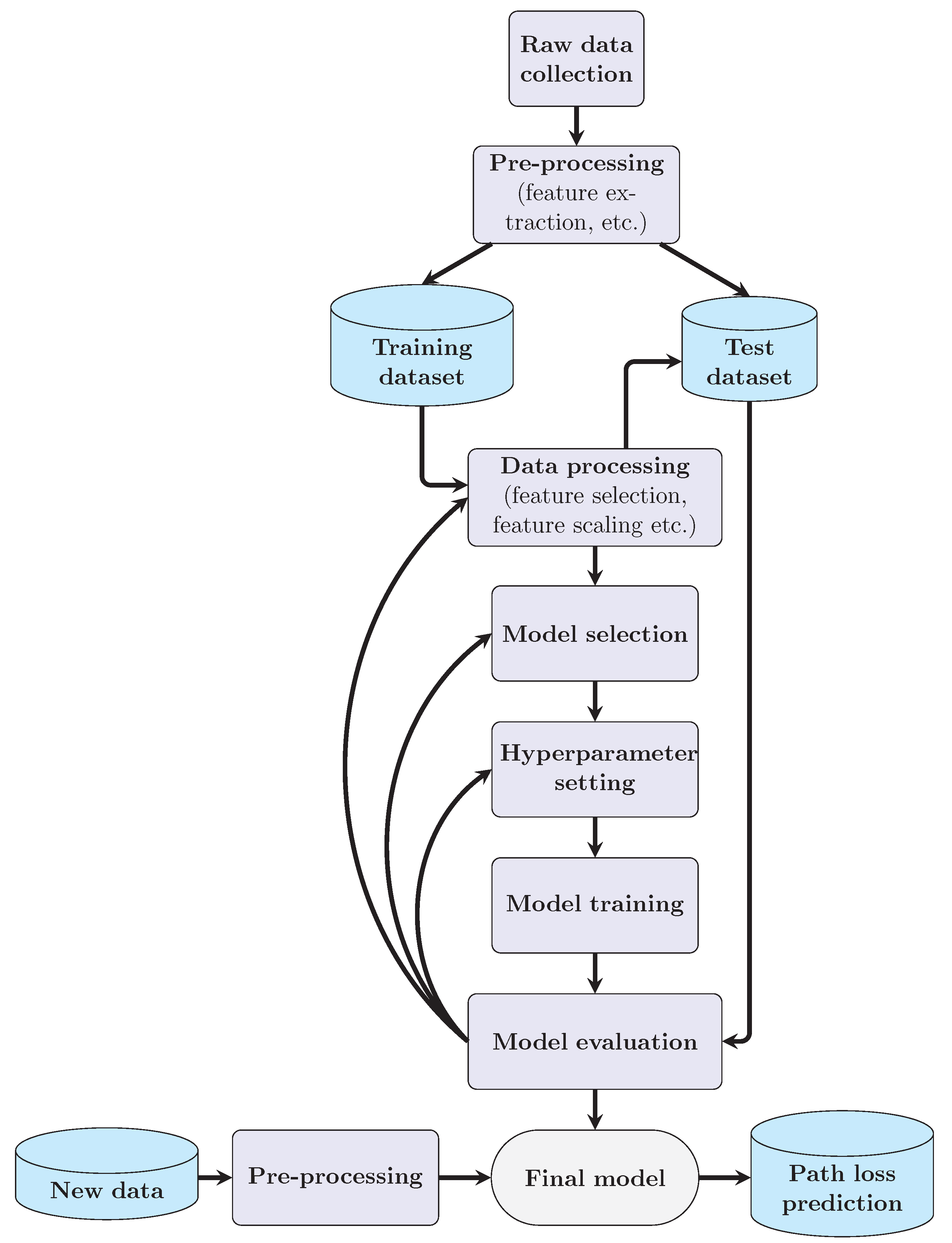
The basic principle of path loss predictors based on machine learning is shown in Figure 1. After knowing the output (path loss observation) and the corresponding input features such as antenna-separation distance and frequency, we can employ machine learning methods to find a good estimation function for the path loss prediction. This function is to map input features to output path loss value, and it can be either a white box (within decision-tree-based models) or a black box (within SVR-based or ANN-based models). The procedure of machine-learning-based path loss predictors is shown in Figure 2 and is introduced step by step as follows.
2.1. Data Collection and Feature Extraction
The collected data refer to samples obtained from measurement, and each sample should include the path loss value and the corresponding input features. The input features can be divided into two categories, system-dependent parameters and environment-dependent parameters. System-dependent parameters are those independent of the propagation environment, such as carrier frequency, heights and positions of the transmitter and receiver, and so on. According to the above parameters, more system-dependent features can be acquired, such as the antenna-separation distance and the angle between the line-of-sight path and the horizontal plane.
Environment-dependent parameters are those determined by the geographic environment and the weather conditions. Parameters related to the geographic environment include the terrain, building conditions, and vegetation conditions. Most of them can be obtained from three-dimensional (3D) digital maps, topographic databases, and land cover databases. The weather parameters include temperature, humidity, precipitation rate, and so on.
The performance of the path loss model is closely related to the number of training samples. After obtaining enough data, these samples should be divided into the training dataset and the test dataset. The former is used to build the prediction model, whereas the latter is used to verify and further improve the model performance.
2.2. Feature Selection and Scaling
In practice, the data used for machine learning may contain hundreds of features. Leaving out relevant features or retaining irrelevant features can both lead to poor quality of the predictor. The goal of feature selection is to select the optimal subset with the least number of features that most contribute to learning accuracy [25].
According to the relationship between feature selection process and model design, there are usually three alternative feature selection approaches, including filter, wrapper and embedded. The filter approach is independent of the proposed model when evaluating feature importance. The wrapper approach takes the prediction performance into account when calculating the feature scores. The embedded approach combines feature selection and the accuracy of the prediction into its procedure [26]. For different algorithms, the stopping conditions are related to the selection of the search algorithm, the feature evaluation criteria, and the specific application requirements.
Some machine-learning-based algorithms, such as ANN, SVR, and KNN, are sensitive to the scale of the input space. Thus, normalization process should be finished before the training begins. That is, all input features and path loss values should be changed in the range from to 1 or from 0 to 1. The normalization method chosen in this paper is the same as that in [7]. It can be expressed as
where x is the value that needs to be normalized, represents the minimum value of the data range, represents the maximum value of the data range, is the value after normalization. The predicted values can be obtained by anti-normalized according to the normalization method.
In contrast, the feature scaling is not required by decision-tree-based methods.
2.3. Model Selection
Different models can be used for the path loss prediction, and the model selection should consider about requirements of both accuracy and complexity. As examples, we will introduce ANN, SVR, and decision tree in Section III. It has been reported that these algorithms have good performance in predicting path loss values [5,20,23].
2.4. Hyperparameter Setting and Model Training
Hyperparameters refer to the parameters whose values are set before the learning process begins. Typical hyperparameters include the number of hidden layers and neurons in ANN, the regularization coefficients and parameters in kernel function of SVR, the tree depth and the size of the ensemble in decision-tree-based algorithms, etc. A set of optimal hyperparameters should be carefully chosen in order to optimize the performance and effectiveness of the path loss prediction. The optimization methods for hyperparameters mainly include grid search, random search, and Bayesian optimization. In this paper, the final values of hyperparameters were obtained by using grid search method. It is an exhaustive search method which takes the best performing parameters as the final result by traversing all the possible values of the parameters.
Model parameters are those parameters learned from training samples. It is worth mentioning that different learning methods have different model parameters. During the model training process, model parameters such as weights and biases are automatically learned.
2.5. Model Evaluation and Path Loss Prediction
In general, the performance of machine-learning-based path loss models is measured by samples in the test dataset, which do not appear in the model training process. The evaluation metrics include prediction accuracy, generalization property, and complexity.
In terms of evaluating the accuracy, performance indicators like maximum prediction error (MaxPE), mean absolute error (MAE), error standard deviation (ESD), correlation factor (CF), root mean square error (RMSE), and mean absolute percentage error (MAPE) are commonly used [3,6].
Generalization property is to describe the model reusability when the deployment concerns new frequency bands or/and new environment types. The model may have better generalization performance with more data collected from diverse scenarios, such as different terrains, frequencies, and vegetative cover conditions.
The computational complexity is usually evaluated by processing time and memory cost. As an example, the number of iterations and convergence speed during the training phase are the key factors that affect the processing time of ANN.
Based on evaluated results, we can select the machine learning algorithm, adjust the hyperparameters, and further improve the prediction model. After the optimal model has been built, path loss values can be generated with new inputs.
3. Methods for Path Loss Prediction
As mentioned above, any supervised learning algorithm can be used for the path loss prediction. In this section, we will introduce some popular models, such as ANN, SVR, and decision tree, and evaluate their prediction performance by means of the measured data.
3.1. ANN
ANN can be used to solve nonlinear regression problems and has low prediction errors when the sample size is large enough, making it a popular algorithm for path loss prediction [3,5,6,10]. ANNs are networks formed by interconnections between neurons. Based on the neuron model, the feed-forward ANN of multi-layer perceptron structure usually contains an input layer, one or more hidden layers, and an output layer. Neurons are fully connected to those in the next layer by different weights, whereas there is no connection between neurons in the same layer and no cross-layer connection.
The number of hidden layers and the number of neurons determine the network size and have a great impact on the model complexity and accuracy. Unfortunately, how to find a suitable ANN structure for the path loss prediction is still an open problem. In [3], it is shown that a non-complex ANN, such as a feed-forward ANN with one hidden layer and only a few neurons, would probably provide sufficient path loss prediction accuracy for a typical rural macrocell radio network planning scenario. ANNs with several hidden layers and numerous neurons may lead to inferior generalization properties compared with the non-complex structures. This phenomenon is probably caused by overtraining, that is, the model performs very well on data similar to the training dataset but is not flexible enough to favorably adapt to data different from the training data.
Back propagation algorithm is a low-complexity method usually used in training ANNs. This type of network is often referred to as BPNN. The subsequent analysis in this paper is based on a 3-layer BPNN structure with fully-connection between layers. Given a set of training samples as , where is a feature vector and is the target output, measured value of path loss. In the forward propagation phase, the predicted value of path loss can be expressed as
where represents the connection weights between the neurons of the hidden layer and inputs, represents the connection weights between the neurons of the output layer and the hidden layer, and are thresholds of the neurons of hidden layer and the neuron of output layer, respectively. and are transfer functions for the neurons in hidden layer and the neuron in output layer, respectively.
The error originating at the output neuron propagates backward. The learning phase of the network proceeds by adaptively adjusting the weights based on the loss function, which is expressed as
where E is the mean squared error.
The back propagation algorithm is based on the gradient descent strategy. Standard gradient descent has some drawbacks, such as slow convergence speed and local poles. Thus, other training methods may also be taken into account, such as Levenberg-Marquardt method, Fletcher-Reeves update method, and Powell-Beale restart method. Among them, the Levenberg-Marquardt algorithm is commonly used for path loss prediction because it has a fast convergence speed at the expense of memory consumption [3,6].
3.2. SVR
Support vector machine (SVM) is a kind of machine learning method based on statistical learning theory. The basic idea of SVM is to nonlinearly map a set of data in the finite-dimensional space to a high-dimensional space such that the dataset is linearly separable. As an extension of SVM, SVR is designed to solve regression problems, so it can be used for path loss prediction [20].
The main idea of SVR is to fine a hyperplane in the high-dimensional feature space to make the sample points fall on it. The hyperplane in the feature space can be described by the following linear function.
where is the normal vector which determines the direction of the hyperplane, is an input feature vector, is the nonlinear mapping function, and b is the displacement item.
The solution to the optimal hyperplane is a constrained optimization problem, which can be written as [27]
where C is regularization coefficient, is insensitive loss which means the predicted value can be considered accurate if the deviation between the predicted value and the actual value is less than , and are the slack variables which allow the insensitivity range on both sides of the hyperplane to be slightly different.
Then, by introducing Lagrange multipliers and solving its dual problem, the approximate function can be expressed as
where and are Lagrange multipliers, and is a kernel function, which is used to perform the nonlinear mapping from the low-dimensional space to the high-dimensional space.
The choice of the kernel function is the key to the performance of the SVR-based predictor. At present, the most common kernel functions include the linear kernel, polynomial kernel, Gaussian radial basis function, sigmoid kernel, and their combinations. In this paper, Gaussian kernel with a tunable parameter is chosen as the kernel function and it is defined by
The Gaussian kernel is a commonly used kernel function [17,18,19,20], which is suitable for tasks with small feature dimensions and lack of prior knowledge. The parameters including regularization coefficient, insensitive loss, and the kernel function parameter in this study were searched as the same method in [20].
3.3. Decision Tree
A decision tree usually contains a root node, some internal nodes, and some leaf nodes. A single decision tree model often has overfitting risk. Thus, new algorithms based on decision tree are proposed, such as AdaBoost and RF [23]. Here, we put the focus on the descriptions of RF.
RF is a machine learning method that combines decision tree and bagging. It applies bootstrap aggregating to each decision tree learner for training samples selection. Furthermore, the random selection of features is introduced in tree training, which means just a set of features is randomly selected for each node split. Therefore, RF is less affected by sample disturbance and feature disturbance, and has higher generalization performance.
For path loss prediction, the predicted value of new samples can be made by averaging the predictions from all the individual decision tree, which is expressed as
where T is the number of decision tree learner, is the prediction of the tth decision tree learner.
3.4. Comparison of Different Models
The BPNN-based model can fully approximate the complicated nonlinear relationship, whereas many parameters need to be selected. In addition, it is difficult to explain the learning process and predicted results.
The SVR-based model is flexible because we can get different models by choosing different kernel functions and different parameters. This flexibility theoretically ensures that the model has strong generalization ability. Besides, the complexity of the model does not depend on the dimension of the input features, avoiding the curse of dimensionality. The main weaknesses of the SVR-based method are the kernel definition and its computational complexity.
The meaning of the decision tree is easy to understand and explain. As an example, RF-based algorithm can provide a natural ranking of features in the model. This advantage is good for the feature selection. Nevertheless, the decision tree often ignores the correlation between the features.
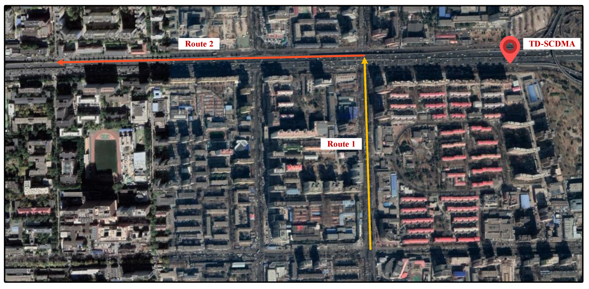
In order to evaluate the performance of these machine learning models, a measurement campaign was carried out in an urban macrocell scenario in Beijing, China. Figure 3 shows the top view of the measurement routes. The considered scenario mostly consists of buildings lower than ten stories. There were also large pedestrian bridges and road signs sparsely distributed, and an average tree density of roughly 6 m high along both sides of the roads.
The received signals from a TD-SCDMA BS at the operating frequency of 2021.4 MHz in this area were considered. The antenna height of the TD-SCDMA BS was about 40 m over the ground. The measurements were made with cars driving on roads in this urban area. An omni-directional receive antenna was mounted on the top of the car roof and connected to a drive-test equipment. The drive-test equipment can record the received signal power and the location information through an external GPS module. Then, the path loss values can be calculated in the offline post-processing and mapped to locations. More details of the equipment can be found in [28].
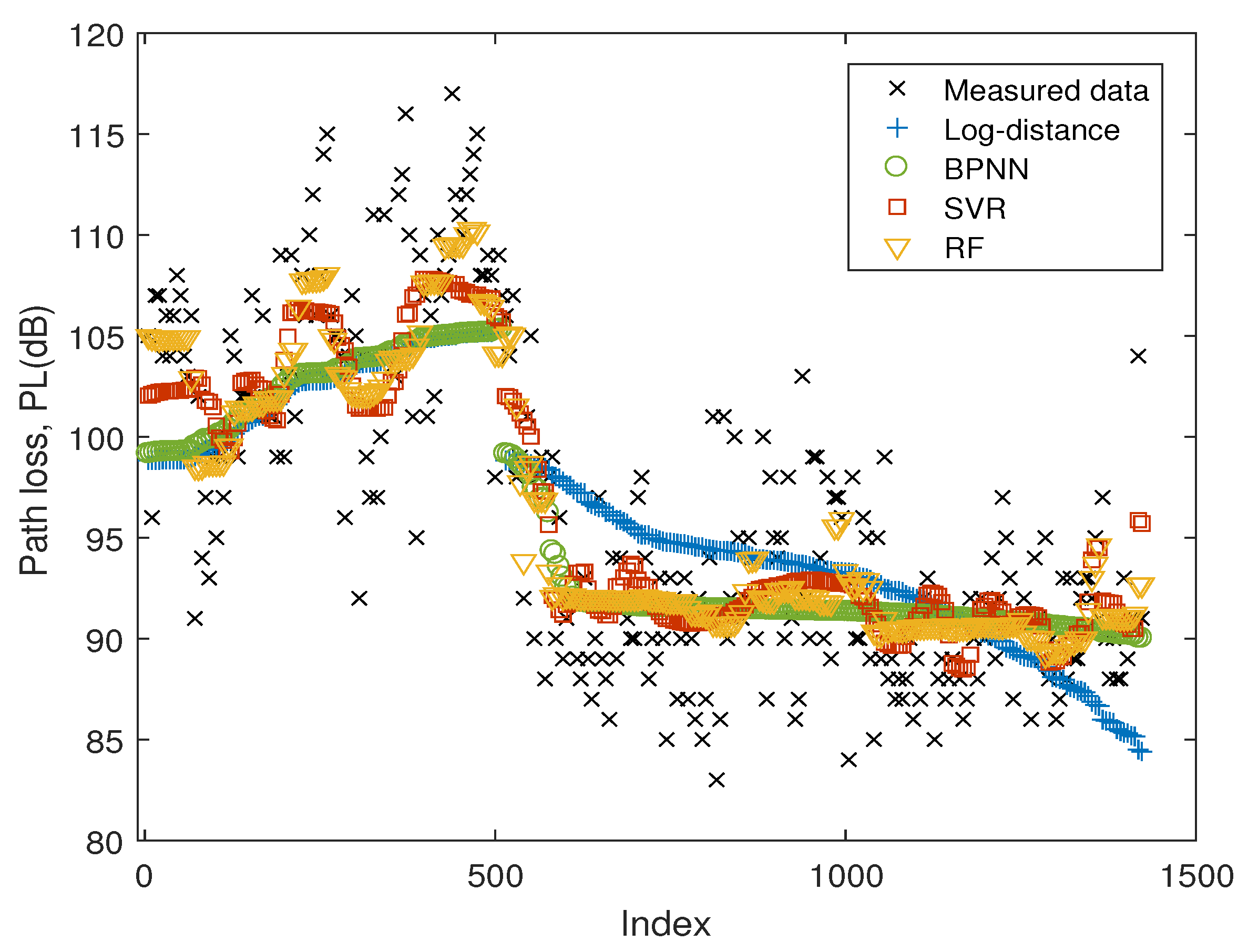
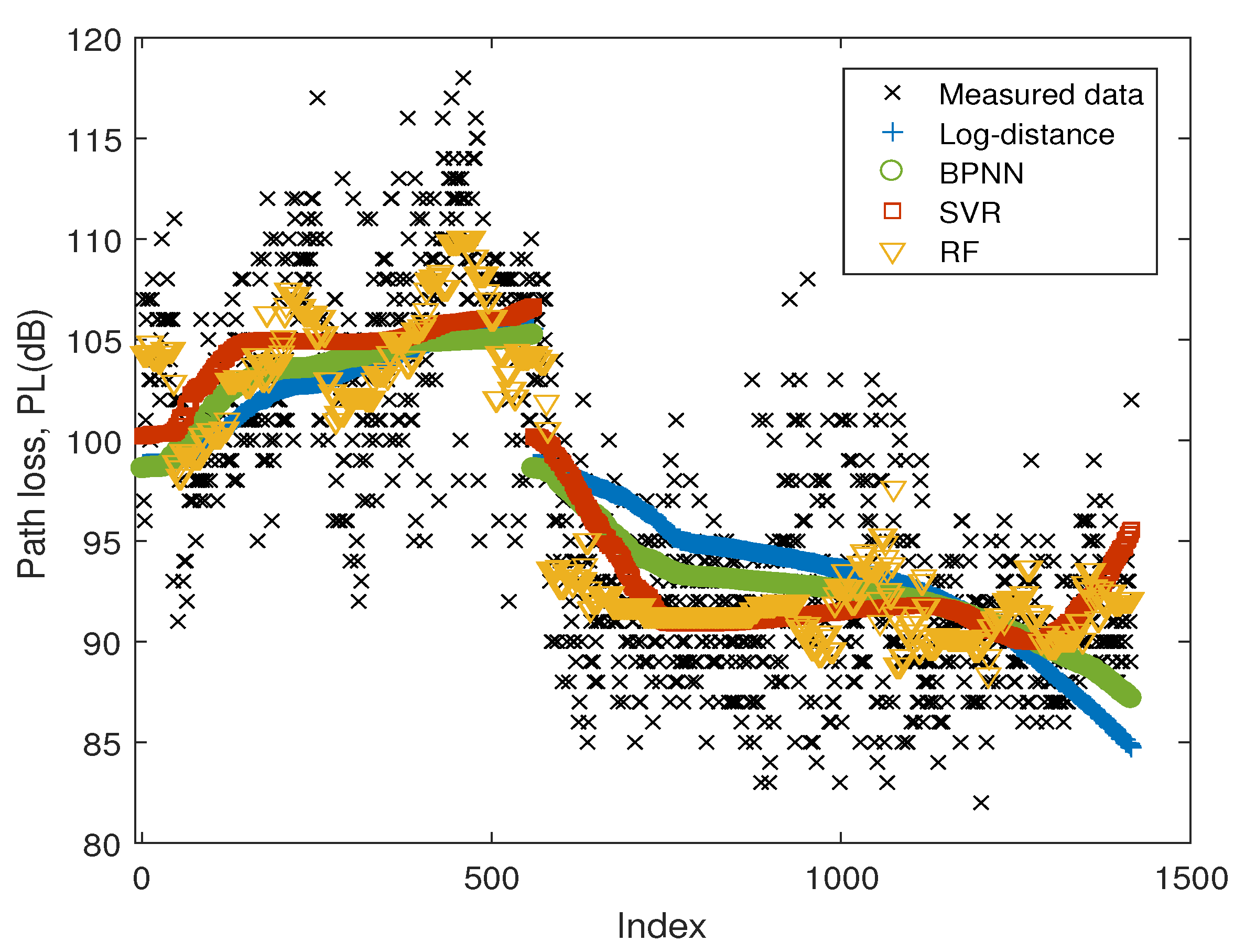
The measurement routes and the position of the TD-SCDMA BS are illustrated in Figure 3. The car moved from the south (sample index 1) to the north (sample index 517), and then turned to the west direction. The total number of collected samples through the two routes was 1483. Each sample included a path loss record and an antenna-separation distance which was calculated according to the GPS information. The antenna-separation distance was used as a single feature. We randomly selected 80% of samples as the training dataset and the remaining 20% as the test dataset. Three aforementioned models, including BPNN, SVR, and RF, were used to predict the path loss values in the test dataset. For BPNN, rectified linear unit function was selected as the activation function. A three-layer feed-forward structure was employed and the optimal number of neurons in the hidden layer was 15. The Gaussian radial basis function was used as the kernel in the SVR-based model. Regularization coefficient, insensitive loss, and the kernel function parameter are set to 451, 91, and 0.25. As the hyperparameters used in RF-based model, the maximum tree depth was 5 and the number of ensemble members was 150. The log-distance model was also considered for comparison.
Figure 4 illustrates the measured data and the predicted results of different models. The x-axis represents the index of test samples, which is corresponding to the positions in the route along the driving direction as shown in Figure 3. As can be observed, the path loss values of Route 1 were higher than those of Route 2. The reason may be that in Route 1, the receive antenna was mainly under non-line-of-sight conditions due to the obstructions of buildings and trees. In contrast, the line-of-sight path played a dominant role in Route 2.
The path loss values at all positions in the test dataset were predicted by using different models. Then, these values were compared with the measured data and the prediction errors were computed. Multiple metrics including RMSE, MAPE, MAE, MaxPE, and ESD were used to evaluate the performance of the predictors, which were expressed as
where is the index of the test sample, Q is the total number of test samples, is the measured data, and is the predicted value of path loss.
The prediction errors of different predictors are listed in Table 1. It is proved that the machine-learning-based models all have good performance and outperform the log-distance model. With selected hyperparameters, RF has the best performance in the measured scenario, followed by SVR, BPNN, and log-distance model.
4. Data Expansion: How to Get Enough Data?
As mentioned, the performance of the machine-learning-based models heavily relies on the amount of data. Here, we propose two schemes to expand the training dataset.
4.1. Data Transferring
One direct way is to utilize the existing data acquired at other frequencies or in other scenarios. Data collected from a similar environment can be adopted for the training purpose. If the generalization capability of the machine-learning-based model is good enough, data from other environments can also be involved.
Nowadays, new frequency bands are continually exploited in wireless communication systems. In empirical models like the path loss model used in WINNER II [29], a frequency-dependent component is added to make the path loss model suitable for a given frequency range. Machine-learning-based models provide another solution, which can involve the frequency as one input feature. Then, the measured data at a known frequency can also be used for training. It should be noted that the frequency difference cannot be too large. Otherwise, the different mechanisms of electromagnetic wave propagation may affect the model performance.
The feasibility of this data transferring method has been verified by measured data from different frequencies and different scenarios. Besides the aforementioned TD-SCDMA BS, we considered two more BSs, including an IS-95 BS and a WCDMA BS. These three BSs were at different positions within a 6 km diameter. The measured routes were different from those in Figure 3, but all the route were selected in similar urban scenarios. The operating frequencies of the IS-95 and WCDMA BSs were 877.26 MHz and 2127.6 MHz, respectively. The same equipment was used to collect received power values and locating information.
We collected 659 samples from the IS-95 BS and 416 samples from the WCDMA BS. All these samples were used as training data. Meanwhile, only 20% samples from TD-SCDMA BS were used for training purpose and the remaining ones were put into the test dataset. After hyperparameter optimization, a three-layer BPNN with 20 neurons in the hidden layer was built. In the SVR-based model, the Gaussian radial basis function was selected as the kernel. Regularization coefficient, insensitive loss, and the kernel function parameter are 491, 21, and 0.25. In the RF-based model, we finally set the maximum tree depth to 7, the number of ensemble members to 14, and maximum 2 features for each split. For comparison, a frequency-dependent component was added to the log-distance model in the same way as [29].
The predicted results of different models on the test dataset are illustrated in Figure 5, and the measured path loss values are also shown for comparison. Again, different metrics are employed to evaluate the prediction error. As illustrated in Table 2, the RMSEs of BPNN, SVR, RF, and log-distance models are 4.74 dB, 4.54 dB, 4.19 dB, and 5.10 dB. With most of the training data from other environments and frequencies, machine-learning-based models can still get satisfactory performance at a new frequency and within different routes.
It should be noticed that limited to the restriction of measured data, only antenna-separation distance and frequency are used as input features. Both of them are important parameters in the path loss modelling and are included in many standardized models, e.g., WINNER I [30], WINNER II [29], WINNER+ [31], and IMT-Advanced (IMT-A) [32] channel models. With these features, our simulation results have already shown that these machine-learning-based models agree well with measured data.
4.2. Combination with Classical Models
Classical models are still valuable for path loss prediction, and they can also be combined with machine-learning-based models. In [33,34], the classical models were employed for the error compensation of machine learning algorithms. Actually, classical models can also be utilized to expand the training dataset.
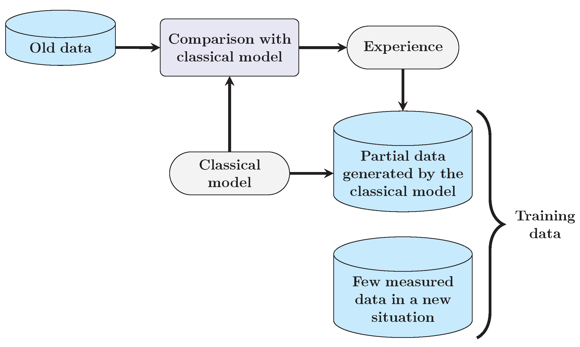
In 5G communication applications, more and more new frequency bands have been introduced. It is very time-consuming and costly to obtain a large amount of measured data at these new frequencies in a short time. It means there would not be no or very limited measured data can be used for modeling. Faced with this challenge, we offer a scheme that employs classical models to generate some training samples. Due to the limitations of accuracy and complexity, it may not be a good choice to directly generate all data samples from classical models and use them for training. The usage of classical models should also be on the basis of the prior information obtained from measured results.
The procedure of this scheme is shown in Figure 6. Firstly, at known frequencies, the measured path loss values are compared with those predicted by the classical model. Then, we can find the positions where predicted results fit the measured data well. It means that at these positions the classical model can approximatively characterize the propagation mechanism. If the new frequency point is not far from the old ones, we can generate path loss values at these positions by classical model and insert them into the training dataset together with the measured values at the old frequencies.
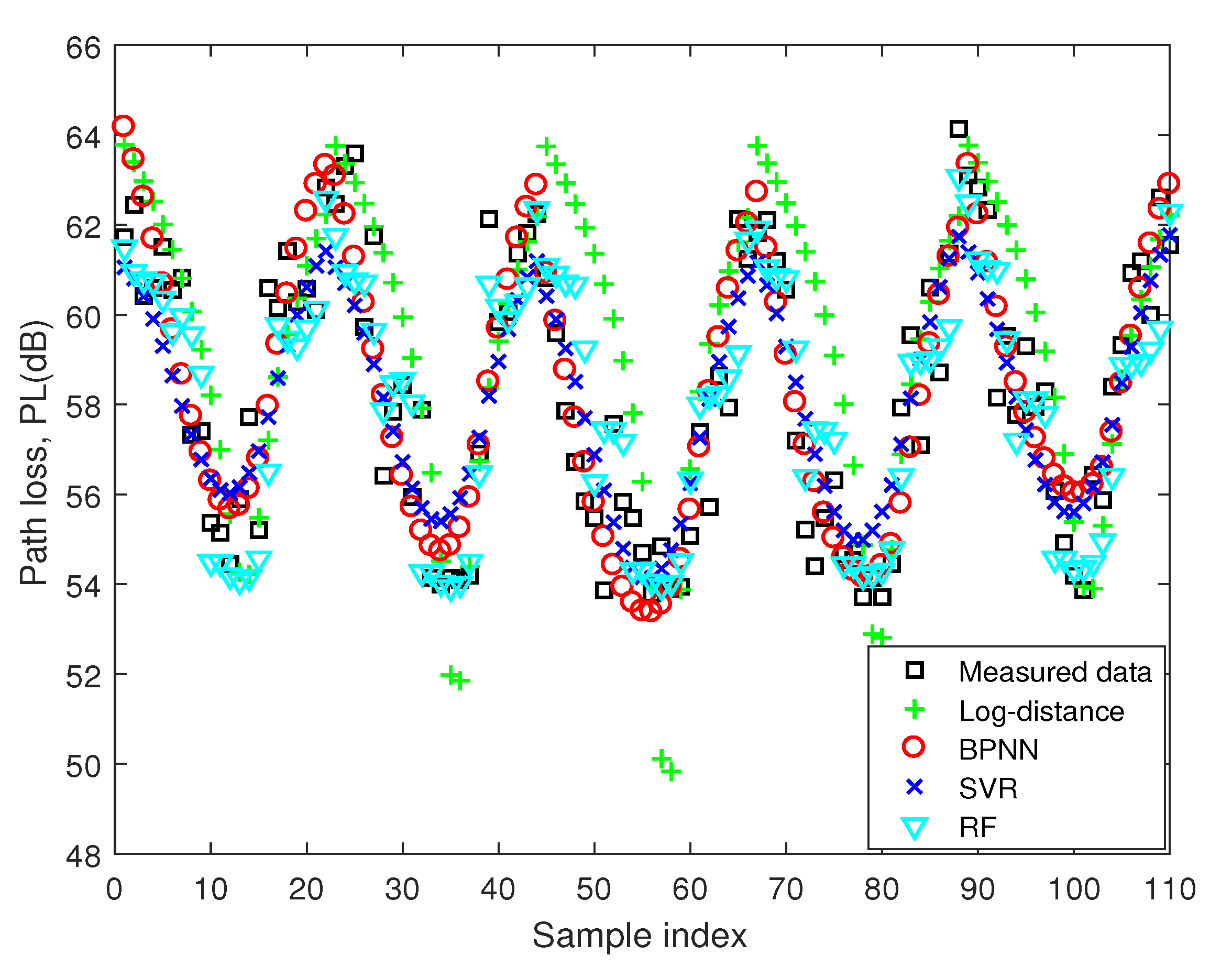
To show the feasibility of this scheme, we considered an aircraft cabin scenario in which path loss data were collected [35]. Three frequencies including 2.4 GHz, 3.52 GHz, and 5.8 GHz were taken into account. At each frequency we got 110 samples from 5 rows with 22 seats in each row. Each sample included a path loss value and two input features (frequency and antenna-separation distance).
Through comparing the log-distance model with the measured data at 2.4 GHz and 3.52 GHz, we chose 30 positions with the smallest fitting errors. Then, path loss values at these positions were estimated by the log-distance model at 5.8 GHz and were added to the training dataset, together with those samples at 2.4 GHz and 3.52 GHz. All measured samples at 5.8 GHz were used for test purpose without participating in the training process.
For BPNN, there were 4 neurons in the hidden layer with hyperbolic tangent sigmoid function as active function. In the SVR-based model, the regularization coefficient and parameter in the Gaussian radial basis kernel function are both 1. The insensitive loss is set as 0.125. For RF, the tree depth and the number of ensemble members were set as 6 and 20, respectively.
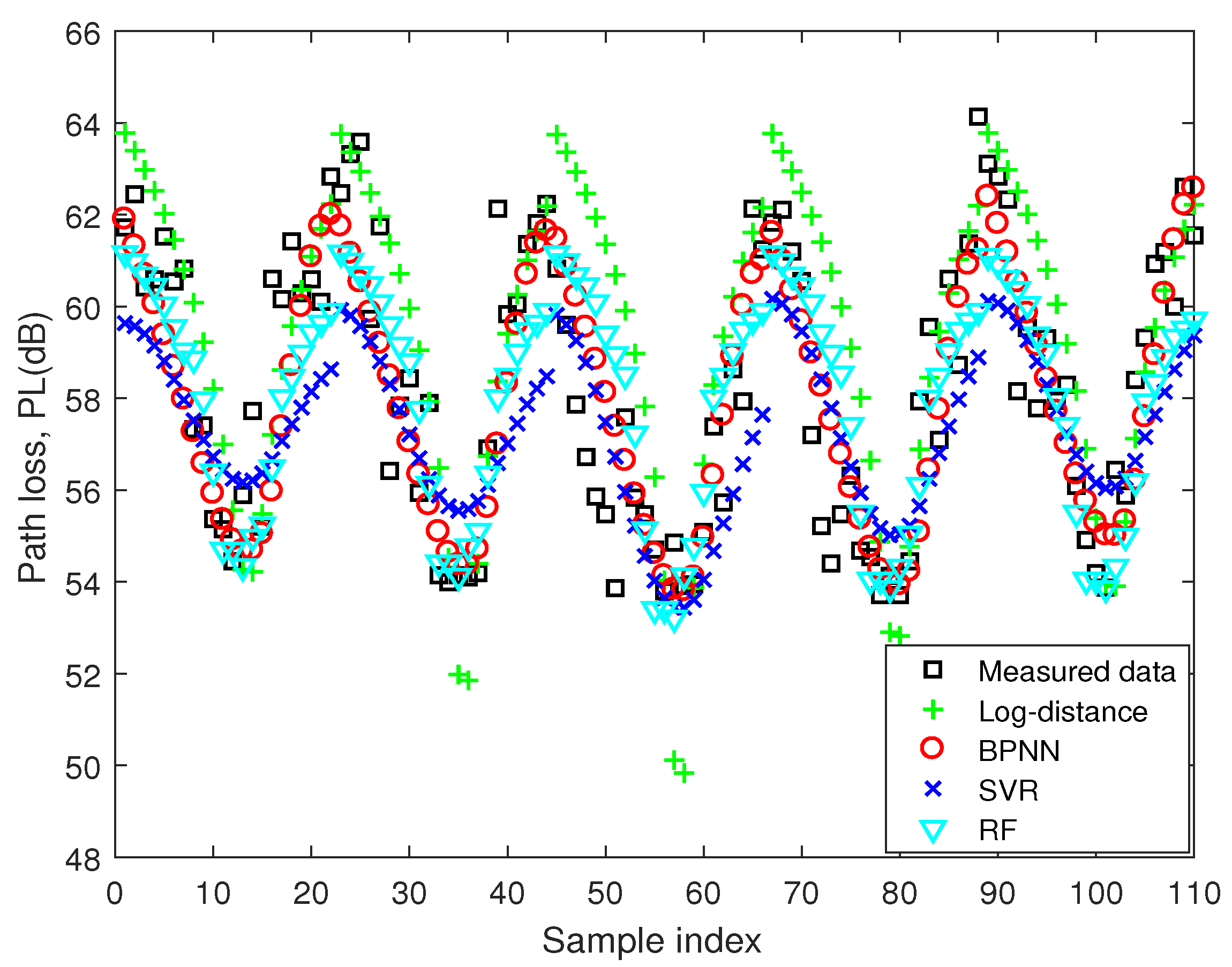
The predicted results for 110 test samples at 5.8 GHz are shown in Figure 7. Although no sample at 5.8 GHz is used for training, these machine-learning-based models are in good agreement with measured data at this frequency. The RMSEs of BPNN, SVR, RF, and log-distance models are 1.61 dB, 2.24 dB, 1.90 dB, and 2.52 dB. The machine-learning-based models still outperform the log-distance model. It is proved that the proposed scheme can be useful for expanding the training dataset even when there is no measured data at a new frequency.
In addition, we selected 6 seats from each row and added these 30 measured samples at 5.8 GHz to the training dataset, together with the data at two known frequencies and those generated by the log-distance model. The hyperparameters were the same as those when no measured data at 5.8 GHz were involved in the training dataset. Then, the predicted path loss values at all 110 seats are shown in Figure 8. The remaining 80 samples in the test dataset are employed for evaluation. The RMSEs of BPNN, SVR, and RF are 1.37 dB, 1.51 dB, and 1.72 dB. It means that the performance of these machine-learning-based models can be further improved if partial measured data at a new frequency have been obtained and utilized for training [35]. This result shows that the prediction accuracy of the model is related to the number of samples. The proposed scheme can effectively expand the training set so as to obtain more samples that reflect the propagation laws at the new frequency.
When a new frequency band is adopted in a wireless communication system, it is hard to collect enough data in a short time. With historical data at known frequencies or only a few data at the new frequency, large deviations in the prediction results are likely to happen due to the bias of the training dataset. Therefore, it is beneficial to provide more data at the new frequency to help find the propagation laws and to improve the prediction accuracy. It has been shown that using the classical models to generate partial channel data is an efficient solution for reducing the prediction inaccuracy caused by data bias. Based on the above results, it can be concluded that this data-expansion method can provide new ideas for quick and efficient path loss prediction at new frequencies. The method may be also helpful to reduce the cost and improve the efficiency of wireless communication planning and deployment.
5. Opportunities for Further Research
5.1. Collection of Training Data
It has been noted that obtaining enough training data is crucial for the accuracy and generalization of the machine-learning-based model. Considering the cost of carrying out measurement campaigns, the question is how many samples are enough for a given prediction accuracy. Evaluation metrics and tools need to be developed for judgment.
Meanwhile, what we need may not be “bigger data”, but “better data”. The diversity and uniformity of the samples should be considered. In a single scenario, the data should be evenly distributed in the measured region. To build a model with good generalization property, measurement routes should be carefully designed to acquire enough data in different scenarios. Therefore, the methodology of channel measurement should be carefully considered.
Additionally, we have offered two schemes to make the most use of existing measured data and classical models. Similar methods can also be investigated to enlarge the training dataset in the future.
5.2. Feature Selection Methodology
Too few features may affect the generalization ability of the path loss predictor. In the above analysis, only system-dependent parameters like antenna-separation distance and frequency are selected as features. It has been shown that these machine-learning-based models agree well with measured data. With limited generalization property, they may be only suitable for similar urban scenarios. Moreover, the usage of more features may not mean better performance. Too many features not only increase the computational requirement, but also probably cause the curse of dimensionality and degrade the prediction performance. Therefore, methodologies need to be developed to guide the feature selection for the path loss predictors based on machine learning.
5.3. Hyperparameter Optimization Problem
Hyperparameter optimization is one of the hardest problems in machine learning. For example, the selection of kernel determines the final performance of SVR-based prediction models. As for ANN-based methods, the number of hidden-layers and the number of neurons are also crucial. Although approaches like grid search can be used for solving this problem to some degree, further research works are still necessary.
5.4. More Machine-Learning-Based Models
With the rapid development of machine learning, new algorithms emerge to improve the model accuracy and computational efficiency. More models and parameters should be taken into consideration to solve the path loss prediction problem.
5.5. Incremental Learning
Until now, machine-learning-based algorithms for path loss prediction are almost based on batch learning, which assumes that all training samples are available before the training. After learning from these samples, the training process is terminated and the model building is finished. However, in practical applications, training samples of path loss increase gradually over time. After new samples arrive, relearning process with all the data takes considerable amount of time and space.
Incremental learning algorithms can gradually update, correct, and enhance previous knowledge so that the updated one can adapt to new arriving samples without relearning from all the data. New knowledge can be learned from the new data to build a more accurate path loss predictor, whereas most of the previous-learned knowledge is retained. However, the accuracy of the path loss predictor may be negatively affected by introducing incremental learning algorithms, which lack the forgetting mechanism for selecting training data.
6. Conclusions
With the development and deployment of 5G networks, network planning puts forward higher requirements on the accuracy, complexity, and versatility of path loss prediction. Machine learning methods, especially supervised learning, can model hidden non-linear relationships and thus can be used for path loss prediction. Based on historical data, machine-learning-based models can build relationship between path loss and input features. It has been shown that machine-learning-based models, including ANN, SVR, and RF, are in good agreement with measured data. In order to satisfy the demand for training data, two data expansion schemes have been proposed to make full use of existing data and classical models. Through the measured data, the feasibility of the proposed schemes has also been verified. Finally, we have summarized the problems still faced by the machine-learning-based path loss prediction.
Author Contributions
Conceptualization, Y.Z. and J.W. (Jing Wang); methodology, Y.Z. and Z.H.; software, J.W. (Jinxiao Wen), and G.Y.; validation, Y.Z., J.W. (Jinxiao Wen), G.Y., and Z.H.; formal analysis, Y.Z.; investigation, J.W. (Jinxiao Wen), and G.Y.; writing—original draft preparation, Y.Z., J.W. (Jinxiao Wen), and G.Y.; writing—review and editing, Y.Z., J.W. (Jinxiao Wen), G.Y., and Z.H.; supervision, Z.H.
Funding
This work was supported in part by National Natural Science Foundation of China (Nos. 61201192, 61871035) and National High Technology Research and Development Program of China (No. 2015AA01A706).
Acknowledgments
We would like to dedicate this paper to Jing Wang, who unfortunately passed away just before the paper was submitted for publication. Wang played an essential role in the research described here and he is greatly missed.
Conflicts of Interest
The authors declare no conflict of interest.
References
- Rappaport, T.S. Wireless Communications: Principles and Practice, 2nd ed.; Prentice-Hall: Upper Saddle River, NJ, USA, 2002. [Google Scholar]
- Phillips, C.; Sicker, D.; Grunwald, D. A survey of wireless path loss prediction and coverage mapping methods. IEEE Commun. Surv. Tutor. 2013, 15, 255–270. [Google Scholar] [CrossRef]
- Östlin, E.; Zepernick, H.J.; Suzuki, H. Macrocell path-loss prediction using artificial neural networks. IEEE Trans. Veh. Technol. 2010, 59, 2735–2747. [Google Scholar] [CrossRef]
- Erceg, V.; Greenstein, L.J.; Tjandra, S.Y.; Parkoff, S.R.; Gupta, A.; Kulic, B.; Julius, A.A.; Bianchi, R. An empirically based path loss model for wireless channels in suburban environments. IEEE J. Sel. Areas Commun. 1999, 17, 1205–1211. [Google Scholar] [CrossRef]
- Ayadi, M.; Zineb, A.B.; Tabbane, S. A UHF path loss model using learning machine for heterogeneous networks. IEEE Trans. Antennas Propag. 2017, 65, 3675–3683. [Google Scholar] [CrossRef]
- Isabona, J.; Srivastava, V.M. Hybrid neural network approach for predicting signal propagation loss in urban microcells. In Proceedings of the 2016 IEEE Region 10 Humanitarian Technology Conference (R10-HTC), Agra, India, 21–23 December 2016; pp. 1–5. [Google Scholar]
- Wu, D.; Zhu, G.; Ai, B. Application of artificial neural networks for path loss prediction in railway environments. In Proceedings of the 2010 5th International ICST Conference on Communications and Networking, Beijing, China, 25–27 August 2010; pp. 1–5. [Google Scholar]
- Popescu, I.; Nikitopoulos, D.; Constantinou, P.; Nafornita, I. ANN prediction models for outdoor environment. In Proceedings of the 2006 IEEE 17th International Symposium on Personal, Indoor and Mobile Radio Communications, Helsinki, Finland, 11–14 September 2006; pp. 1–5. [Google Scholar]
- Popescu, I.; Nikitopoulos, D.; Nafornita, I.; Constantinou, P. ANN prediction models for indoor environment. In Proceedings of the 2006 IEEE International Conference on Wireless and Mobile Computing, Networking and Communications, Montreal, QC, Canada, 19–21 June 2006; pp. 366–371. [Google Scholar]
- Zineb, A.B.; Ayadi, M. A multi-wall and multi-frequency indoor path loss prediction model using artificial neural networks. Arabian J. Sci. Eng. 2016, 41, 987–996. [Google Scholar] [CrossRef]
- Ayadi, M.; Zineb, A.B. Body shadowing and furniture effects for accuracy improvement of indoor wave propagation models. IEEE Trans. Wirel. Commun. 2014, 13, 5999–6006. [Google Scholar] [CrossRef]
- Popescu, I.; Kanstas, A.; Angelou, E.; Nafornita, L.; Constantinou, P. Applications of generalized RBF-NN for path loss prediction. In Proceedings of the 13th IEEE International Symposium on Personal, Indoor and Mobile Radio Communications, Pavilhao Altantico, Lisboa, Portugal, 18 September 2002; pp. 484–488. [Google Scholar]
- Bhuvaneshwari, A.; Hemalatha, R.; Satyasavithri, T. Performance evaluation of Dynamic Neural Networks for mobile radio path loss prediction. In Proceedings of the 2016 IEEE Uttar Pradesh Section International Conference on Electrical, Computer and Electronics Engineering (UPCON), Varanasi, India, 9–11 December 2016; pp. 461–466. [Google Scholar]
- Pedraza, L.F.; Hernández, C.A.; López, D.A. A model to determine the propagation losses based on the integration of hata-okumura and wavelet neural models. Int. J. Antennas Propag. 2017, 2017, 1–8. [Google Scholar] [CrossRef]
- Cruz, H.A.O.; Nascimento, R.N.A.; Araujo, J.P.L.; Pelaes, E.G.; Cavalcante, G.P.S. Methodologies for path loss prediction in LTE-1.8 GHz networks using neuro-fuzzy and ANN. In Proceedings of the 2017 SBMO/IEEE MTT-S International Microwave and Optoelectronics Conference (IMOC), Aguas de Lindoia, Brazil, 27–30 August 2017; pp. 1–5. [Google Scholar]
- Salman, M.A.; Popoola, S.I.; Faruk, N.; Surajudeen-Bakinde, N.T.; Oloyede, A.A.; Olawoyin, L.A. Adaptive Neuro-Fuzzy model for path loss prediction in the VHF band. In Proceedings of the 2017 International Conference on Computing Networking and Informatics (ICCNI), Lagos, Nigeria, 29–31 October 2017; pp. 1–6. [Google Scholar]
- Hung, K.C.; Lin, K.P.; Yang, G.K.; Tsai, Y.C. Hybrid support vector regression and GA/TS for radio-wave path-loss prediction. In International Conference on Computational Collective Intelligence: Technologies and Applicat; Springer: Berlin, Germany, 2010; pp. 243–251. [Google Scholar]
- Lin, K.P.; Hung, K.C.; Lin, J.C.; Wang, C.K. Applying least squares support vector regression with genetic algorithms for radio-wave path loss prediction in suburban environment. In Advances in Neural Network Research and Applications; Springer: Berlin, Germany, 2010; pp. 861–868. [Google Scholar]
- Zhao, X.; Hou, C.; Wang, Q. A new SVM-based modeling method of cabin path loss prediction. Int. J. Antennas Propag. 2013, 2013, 1–7. [Google Scholar] [CrossRef]
- Uccellari, M.; Facchini, F.; Sola, M.; Sirignano, E.; Vitetta, G.M.; Barbieri, A.; Tondelli, S. On the use of support vector machines for the prediction of propagation losses in smart metering systems. In Proceedings of the 2016 IEEE 26th International Workshop on Machine Learning for Signal Processing (MLSP), Vietri sul Mare, Italy, 13–16 September 2016; pp. 1–6. [Google Scholar]
- Zhang, Y.; Wen, J.; Yang, G.; He, Z.; Luo, X. Air-to-Air path loss prediction based on machine learning methods in urban environments. Wirel. Commun. Mob. Comput. 2018, 2018, 1–9. [Google Scholar] [CrossRef]
- Hou, W.; Shi, D.; Gao, Y.; Yao, C. A new method for radio wave propagation prediction based on finite integral method and machine learning. In Proceedings of the 2017 IEEE 5th International Symposium on Electromagnetic Compatibility (EMC-Beijing), Beijing, China, 28–31 October 2017; pp. 1–4. [Google Scholar]
- Oroza, C.A.; Zhang, Z.; Watteyne, T.; Glaser, S.D. A machine-learning based connectivity model for complex terrain large-scale low-power wireless deployments. IEEE Trans. Cogn. Commun. Netw. 2017, 3, 576–584. [Google Scholar] [CrossRef]
- Chen, G.S.; Wang, R.C.; Lu, J.Y.; Xu, Y.R. Intelligent path loss prediction engine design using machine learning in the urban outdoor environment. In Proceedings of the Sensors and Systems for Space Applications, Orlando, FL, USA, 2 May 2018; pp. 1–7. [Google Scholar]
- Khalid, S.; Khalil, T.; Nasreen, S. A survey of feature selection and feature extraction techniques in machine learning. In Proceedings of the 2014 Science and Information Conference, London, UK, 27–29 August 2014; pp. 372–378. [Google Scholar]
- Han, H.; Guo, X.; Yu, H. Variable selection using mean decrease accuracy and mean decrease Gini based on random forest. In Proceedings of the 2016 7th IEEE International Conference on Software Engineering and Service Science (ICSESS), Beijing, China, 26–28 August 2016; pp. 219–224. [Google Scholar]
- Chang, C.C.; Lin, C.J. LIBSVM-A Library for Support Vector Machines. 2003. Available online: http://www.csie.ntu.edu.tw/cjlin/libsvm/ (accessed on 9 May 2019).
- Liang, C.; Li, H.; Li, Y.; Zhou, S.; Wang, J. A learning-based channel model for synergetic transmission technology. China Commun. 2015, 12, 83–92. [Google Scholar] [CrossRef]
- Kyösti, P. IST-4-027756 WINNER II D1.1.2 v1.2 WINNER II channel models. 2008. Available online: http://www.ist-winner.org/WINNER2-Deliverables/D1.1.2.zip (accessed on 9 May 2019).
- Baum, D.S.; El-Sallabi, H.; Jämsä, T.; Meinilä, J. IST-2003-507581 WINNER D5.4 v1.4 Final Report on Link Level and System Level Channel Models. 2005. Available online: http://www.ist-winner.org/DeliverableDocuments/D5.4.pdf (accessed on 9 May 2019).
- Meinila, J.; Kyösti, P.; Hentila, L.; Jamsa, T.; Suikkanen, E.; Kunnari, E.; Narandzia, M.D. 5.3: WINNER+ Final Channel Models, CELTIC/CP5-026, June 2010. Available online: http://projects.celtic-initiative.org/winner+/index.html (accessed on 9 May 2019).
- ITU-R M.2135-1. Guidelines for Evaluation of Radio Interface Technologies for IMT-Advanced. 2009. Available online: http://www.itu.int/pub/R-REP-M.2135/en (accessed on 9 May 2019).
- Milijić, M.; Stanković, Z.; Milovanović, I. Hybrid-empirical neural model for indoor/outdoor path loss calculation. In Proceedings of the 2011 10th International Conference on Telecommunication in Modern Satellite Cable and Broadcasting Services (TELSIKS), Nis, Serbia, 5–8 October 2011; pp. 548–551. [Google Scholar]
- Popescu, I.; Nikitopoulos, D.; Constantinou, P. Comparison of ANN based models for path loss prediction in indoor environment. In Proceedings of the IEEE Vehicular Technology Conference, Montreal, QC, Canada, 25–28 September 2006; pp. 1–5. [Google Scholar]
- Wen, J.; Zhang, Y.; Yang, G.; He, Z.; Zhang, W. Path loss prediction based on machine learning methods for aircraft cabin environment. IEEE Access 2019. submitted. [Google Scholar]
Figure 1.
Principle of machine-learning-based path loss prediction.

Figure 2.
Procedure of machine-learning-based path loss prediction.

Figure 3.
Top view of the measurement routes and TD-SCDMA BS in the urban scenario.

Figure 4.
Prediction performance of different predictors on the test dataset. The samples are from TD-SCDMA BS, with 80% of the samples as training dataset and 20% of the samples as test dataset.
Figure 4.
Prediction performance of different predictors on the test dataset. The samples are from TD-SCDMA BS, with 80% of the samples as training dataset and 20% of the samples as test dataset.

Figure 5.
Prediction performance of different predictors on the test dataset. The samples are from three different BSs, with all samples from IS-95 BS and WCDMA BS and 20% of the samples from TD-SCDMA BS as training dataset and 80% of the samples from TD-SCDMA BS as test dataset.
Figure 5.
Prediction performance of different predictors on the test dataset. The samples are from three different BSs, with all samples from IS-95 BS and WCDMA BS and 20% of the samples from TD-SCDMA BS as training dataset and 80% of the samples from TD-SCDMA BS as test dataset.

Figure 6.
Expansion of training data with the usage of classical model.

Figure 7.
Prediction performance of different models on the 110 samples at 5.8 GHz. For the samples at 5.8 GHz, only 30 estimated samples participate in the training process.
Figure 7.
Prediction performance of different models on the 110 samples at 5.8 GHz. For the samples at 5.8 GHz, only 30 estimated samples participate in the training process.

Figure 8.
Prediction performance of different models on the 110 samples at 5.8 GHz. For the samples at 5.8 GHz, 30 estimated samples and 30 measured samples participate in the training process.
Figure 8.
Prediction performance of different models on the 110 samples at 5.8 GHz. For the samples at 5.8 GHz, 30 estimated samples and 30 measured samples participate in the training process.


Table 1.
Comparison of Prediction Accuracy of Different Predictors on the 20% Test Samples from TD-SCDMA BS.
Table 1.
Comparison of Prediction Accuracy of Different Predictors on the 20% Test Samples from TD-SCDMA BS.
| Metric | BPNN | SVR | RF | Log-Distance |
|---|---|---|---|---|
| RMSE [dB] | 4.65 | 4.21 | 3.93 | 5.28 |
| MAPE [%] | 5.44 | 4.94 | 4.58 | 6.53 |
| MAE [dB] | 0.81 | 0.11 | 0.10 | 0.24 |
| MaxPE [dB] | 13.97 | 12.18 | 12.06 | 19.50 |
| ESD [dB] | 4.59 | 4.22 | 3.94 | 5.29 |
Table 2.
Comparison of Prediction Accuracy of Different Predictors on the 80% Test Samples from TD-SCDMA BS.
Table 2.
Comparison of Prediction Accuracy of Different Predictors on the 80% Test Samples from TD-SCDMA BS.
| Metric | BPNN | SVR | RF | Log-Distance |
|---|---|---|---|---|
| RMSE [dB] | 4.74 | 4.54 | 4.19 | 5.10 |
| MAPE [%] | 5.62 | 5.40 | 4.76 | 6.21 |
| MAE [dB] | 0.29 | -0.26 | 0.26 | 0.01 |
| MaxPE [dB] | 15.27 | 16.70 | 17.94 | 17.27 |
| ESD [dB] | 4.73 | 4.54 | 4.18 | 5.10 |
© 2019 by the authors. Licensee MDPI, Basel, Switzerland. This article is an open access article distributed under the terms and conditions of the Creative Commons Attribution (CC BY) license (http://creativecommons.org/licenses/by/4.0/).
Share and Cite
MDPI and ACS Style
Zhang, Y.; Wen, J.; Yang, G.; He, Z.; Wang, J. Path Loss Prediction Based on Machine Learning: Principle, Method, and Data Expansion. Appl. Sci. 2019, 9, 1908. https://0-doi-org.brum.beds.ac.uk/10.3390/app9091908
AMA Style
Zhang Y, Wen J, Yang G, He Z, Wang J. Path Loss Prediction Based on Machine Learning: Principle, Method, and Data Expansion. Applied Sciences. 2019; 9(9):1908. https://0-doi-org.brum.beds.ac.uk/10.3390/app9091908
Chicago/Turabian StyleZhang, Yan, Jinxiao Wen, Guanshu Yang, Zunwen He, and Jing Wang. 2019. "Path Loss Prediction Based on Machine Learning: Principle, Method, and Data Expansion" Applied Sciences 9, no. 9: 1908. https://0-doi-org.brum.beds.ac.uk/10.3390/app9091908
Note that from the first issue of 2016, this journal uses article numbers instead of page numbers. See further details here.