Testing and Validation of Automotive Point-Cloud Sensors in Adverse Weather Conditions

VTT Technical Research Centre of Finland, P.O. Box 1300, FI-33101 Tampere, Finland
*
Author to whom correspondence should be addressed.
Appl. Sci. 2019, 9(11), 2341; https://0-doi-org.brum.beds.ac.uk/10.3390/app9112341
Submission received: 29 March 2019
/
Revised: 31 May 2019
/
Accepted: 4 June 2019
/
Published: 7 June 2019
(This article belongs to the Special Issue LiDAR and Time-of-flight Imaging)
Abstract
:Light detection and ranging sensors (LiDARS) are the most promising devices for range sensing in automated cars and therefore, have been under intensive development for the last five years. Even though various types of resolutions and scanning principles have been proposed, adverse weather conditions are still challenging for optical sensing principles. This paper investigates proposed methods in the literature and adopts a common validation method to perform both indoor and outdoor tests to examine how fog and snow affect performances of different LiDARs. As suspected, the performance degraded with all tested sensors, but their behavior was not identical.
1. Introduction
The light detection and ranging (LiDAR) sensors are one of the most promising options for automated driving. They provide range and intensity information from their surroundings. From the obtained data, objects can be not only detected, but also recognized (e.g., pedestrians, other vehicles). LiDAR development has been intense in recent years and, for example, their resolution has improved significantly. However, they still have their weaknesses, especially in adverse weather conditions. In order to tackle the automated driving challenges—(1) Objects on the road,(2) traffic jam ahead, (3) pedestrians crossing the road,(4) enhanced environmental awareness, and (5) drivable area awareness in all condition—the performance of LiDARs and their limits need to be investigated, and possibly, solutions need to be found for these restrictions.
Primarily, two kinds of methods have been used to investigate and validate the performance of automotive LiDARs: Mathematical models and simulations, and indoor tests in fog chambers. In both methods, it is easy to reproduce and control the test environment and conditions. Additionally, there is no need to use real vehicles. This saves fuel and working hours, and is safer, especially when considering some risky scenarios in traffic.
In [1], Rasshofer et al. investigated physical principles behind the influence of weather on LiDARs. Based on this, they developed a novel electro-optical laser radar target simulator system. Its idea is to reproduce the optical return signals measured by reference laser radar under adverse weather conditions. It replicates their pulse shape, wavelength, and power levels. Real-world measurements in fog, rain, and snow were performed to verify their models, though this proved to be somewhat challenging as the conditions in real traffic are neither predictable nor stable.
Hasirlioglu et al. [2] presented a model to describe the impact of rain. The distance between object and sensor is divided into layers whose effects (absorption, transmission, and reflection of light) per layer are considered in summary. To validate their theoretical model, they built a rain simulator that was furthermore validated by comparing it to statistical data of real rain.
Fersch et al. investigated the influence of rain on LiDARs with a small aperture [3]. They developed two models to examine the effect of two potentially performance degrading scenarios: Discrete rain drops in the proximity of a laser aperture and a protective window getting wet. In conclusion, neither of the scenarios have a significant effect on LiDARs’ performance.
In [4], Reway et al. presented a hardware-in-the-loop testing method with real automotive cameras, which were connected to a simulated environment. In this environment, they were able to create different traffic scenarios and vary the environmental conditions, including dense fog. The method was eventually used to validate an ADAS platform available on the market. The obtained results matched the specification of the ADAS platform, showing the applicability of the developed testing method.
Goodin et al. developed a mathematical model for the performance degradation of LiDAR as a function of rain-rate [5]. Furthermore, the model was incorporated into a 3D autonomous vehicle simulator which also has a detailed physics-based LiDAR simulation, also known as the Mississippi State University autonomous vehicle simulator (MAVS). According to their tests run in simulations of the obstacle-detection system for roof-mounted LiDAR, heavy rain does not seem to decrease the system’s performance significantly.
Indoor fog chambers are used both for experimentally investigating the performance of sensors [6,7,8,9,10,11] and for validating the developed models against real conditions [1,3]. Many have built their own chamber to mimic fog or rain and some have used the state-of-the-art fog chamber of CEREMA. Depending on the chosen chamber, the methods to modify the parameters of weather conditions inside the chamber (e.g., visibility) vary. In CEREMA’s fog chamber, they have a wide variety of adjustable parameters (fog’s particle size, meteorological visibility, rain’s particle size, and intensity). In self-built chambers, the fog density is primarily controlled by the number of fog layers.
Tests performed in fog chambers are always static, and neither the sensors nor the targets were moving at all. The targets used are usually “natural” targets, i.e., vehicles, mannequin puppets, but calibrated targets were occasionally used [6,7,8].
Hasirlioglu et al. [7] built their own rain simulator that consisted of rain layers that are individually controlled. The rain intensity is adjusted by varying the activated rain layers. By increasing the number of active rain layers, they find the point where the sensor is no longer able to differentiate the target from the rain. This is the basis of their benchmark methodology: The number of rain layers with a specific rain intensity defines the performance of the sensor tested. The rain simulator and methodology can also be used to validate theoretical models. Basic radar, LiDAR, and camera sensors were tested to show the influence of rain on their performance. As a target, they used the Euro NCAP vehicle target, which is a standardized test object.
Hasirlioglu et al. [8] continued their work by creating a fog simulator. Its principle is similar to their rain simulator as it consists of individually controlled fog layers. Sensor disturbance is, again, increased by activating more and more layers. They did not use any glycol or glycerin-based fluid to create the fog, thus ensuring the natural absorption and scattering properties of real fog. The principle for detecting the performance of sensors is also similar to their rain simulator: When the sensor is no longer able to differentiate its target from the fog, its limit is reached. The number of active fog layers serves as the assessment criterion.
In their study, Kim et al. [9] concentrated on how fog affects the visibility of a safety sensor for a robot. Hence, the working environment is not in traffic, but the sensors used are the same as in the traffic environment. In their artificial fog chamber, the density of fog and brightness of the chamber are controlled to meet a desired target value. The laser device measures the spectral transmission. The visibility of Velodyne VLP-16 was investigated visually and their result was that its performance decreases the denser the fog is.
Daniel et al. [10] presented a test setup with a sensor set that consisted of a low-THz imaging radar, a LiDAR, and a stereo optical camera. Their aim is to highlight the need for low-THz radar as a part of automotive sensor setup especially in weather conditions where optical systems fail. They built their own fog chamber inside a large tent in order to maintain a dense fog. The fog was created with a commercial smoke machine. As targets, they had two dummies as pedestrians, a metallic trolley, and a reference target. Visibility was measured with a Secchi disc. They recorded images at three fog density levels. Visually examining the results yielded that fog does not affect the performance of radar much, whereas the visibility of LiDARs and cameras is decreased when fog density increases.
Bijelic et al. [6] had four LiDARs from Velodyne and Ibeo evaluated in CEREMA’s climate chamber, where it is possible to produce two different fog droplet distributions. The density of fog is continuously controlled, thus keeping the fog stable. The test scene consisted of various different targets, e.g., reflector posts, pedestrian mannequins, a traffic sign, and a car. LiDAR sensors were located at their pre-selected positions on a test vehicle, which was placed at the beginning of the chamber. Velodyne sensors were mounted on top of the car and Ibeo sensors at its bumper. The static scene was recorded with different fog densities and droplet distributions with all sensors.
These measurements were visually investigated and resulted in the general conclusion that fog reduces the maximum viewing distance. However, when two manufacturers’ sensors were compared, Ibeo LiDARs were able to detect targets at a lower visibility than Velodyne sensors. Only a small difference was found between advection and radiation fog’s influence, so evaluation was continued using only advection fog (large droplets).
Furthermore, Bijelic et al. further evaluated the performance of their setup by using calibrated Zenith Polymer diffuse-reflective targets with reflectivities of 5%, 50%, and 90%. They were installed on a pole that a person held away from oneself. With this setup, they obtained the maximum viewing distance for each sensor. Again, these measurements even further verify that the fog decreases the maximum viewing distance drastically. Using multiple echoes and adaptive noise levels, the performance is improved but still not to a level that is sufficient for autonomous driving.
In their study, Kutila et al. [11] evaluated and compared LiDARs with two different wavelengths of 950 nm and 1550 nm in the CEREMA fog chamber. Operating wavelength of 1550 nm is justified by its potential benefits: Less scattering in fog and more optical energy can be used because of the more relaxed eye safety regulations. However, in their study, the option for more optical power was ignored and they concentrated on measuring the scattering in fog. To analyze the visibility, they selected targets that represented typical road traffic scenarios: Mannequins as pedestrians, a traffic sign, and a car. Comparison to find out the effect of wavelength was done so that a reference visibility, from which the reference energy was measured, was chosen and reflected energy values at other visibilities were compared to the reference energy. Despite taking into account all the possible differences between the 905 nm and 1550 nm LiDARs, they were not able to find significant differences in the reflected energies.
Filgueira et al. studied the effects of real rain on LiDAR measurements outdoors [12]. They set up Velodyne VLP-16 outside to measure six areas with different materials and surfaces. Rain attribute values were obtained from a nearby meteorological station and they were assumed constant in the area under examination. Performance was evaluated by comparing the range and intensity measurements to a reference situation, i.e., no rain. Their results show variations in range measurements and decreases in returned intensity values as the rain density increases.
Even though the effects of adverse weather are intensely investigated, the studies have concentrated on rain and fog, leaving out other potentially critical weather conditions. For example, the effects of snowfall and powder snow are still unknown, although estimations based on existing knowledge can be made. Still, no artificial snow simulators exist nor are there outdoor tests performed in snowy conditions.
To offset this lack of knowledge, we performed tests with various LiDARs inside a fog chamber and outside in snowy conditions. These tests and their results are presented in the next two chapters. The aim is to keep the testing process practical to meet the major obstacles in roadmap towards automated driving.
2. Materials and Methods
Two types of tests were performed: Indoors in the CEREMA fog chamber and outdoors in northern Finland and Sweden. The sets of sensors were nearly the same in both testing environments.
A set of LiDARs used in tests consisted of Velodyne PUCK VLP-16, Ouster OS-164, Cepton HR80T and HR80W, and Ibeo Lux. In outdoor tests, Robosense RS-LiDAR-32 was also included, but it did not arrive in time for fog chamber tests. A selected set provided a wide range of LiDARs with different designs from various manufacturers. Their specifications are presented in more detail in Table 1. Velodyne, Ouster, and Robosense are of similar design with a cylinder-shaped casing and based on a constantly rotating structure. Cepton’s design differs from this as it uses two mirrors and covers the field of view with a sine wave -like pattern. Other sensors use layers on top of one another to create a vertical view. Ouster operates on a different wavelength (850 nm) than the rest of the sensors, which use wavelengths around 905 nm. All sensors are said to work at sub-zero temperatures but Velodyne and Robosense only as low as −10 °C, which may not be enough for the snowy tests performed in a colder environment.
Fog and rain tests were performed in the Clermont-Ferrand laboratory, where a fog chamber is located. It is a state-of-the-art fog chamber where it is possible to control and reproduce the fog’s particle size, meteorological visibility, and rain’s particle size and intensity [13]. Here, the meteorological visibility means the visibility distance, which is a practical parameter describing fog characteristics in relation to light transmission (see more detailed definition in [13]).
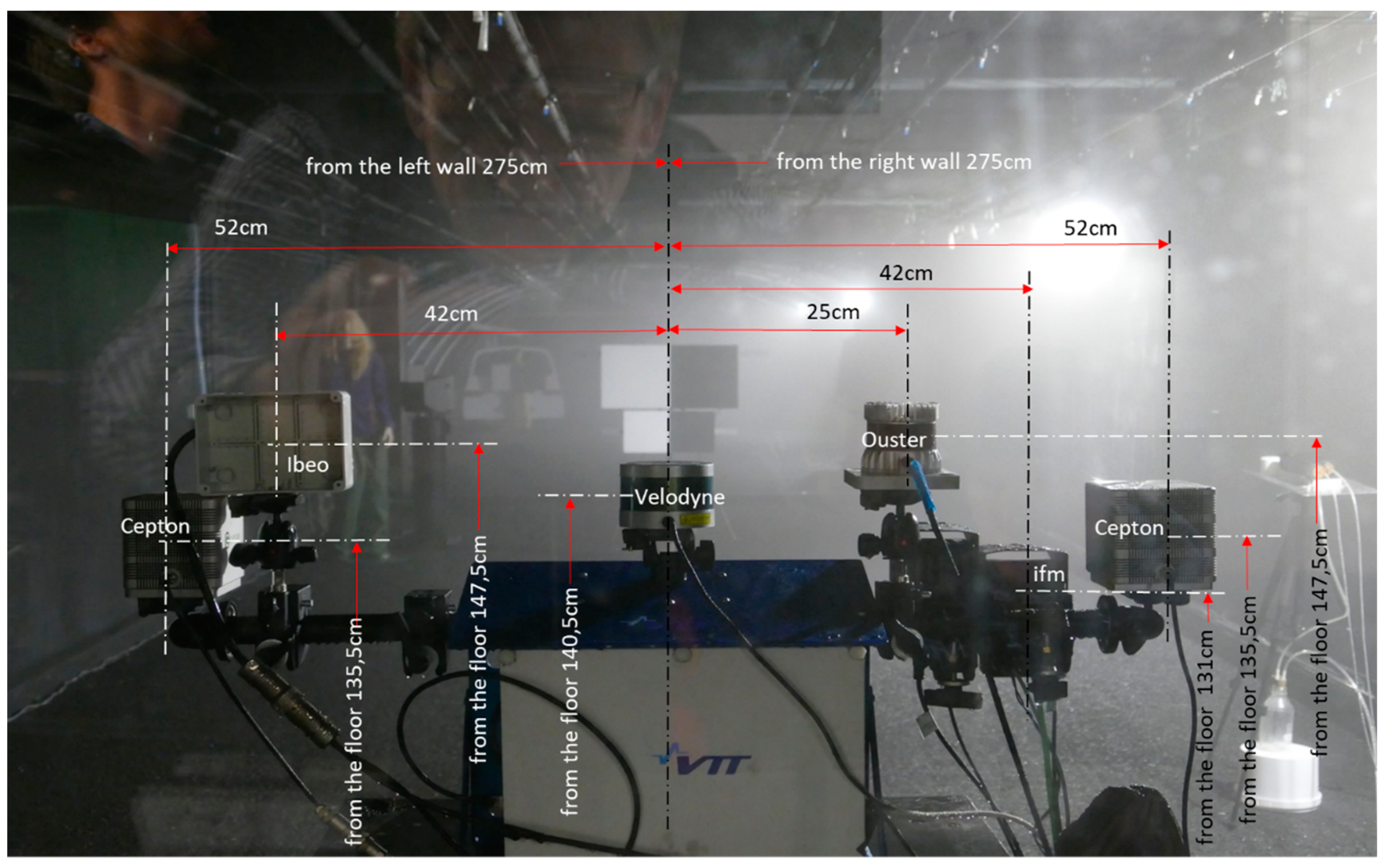
LiDAR performance tests in foggy conditions were executed in late November 2018. LiDARs were mounted side-by-side facing the targets in the tunnel as shown in Figure 1. To reduce interference, only one LiDAR at a time was turned on and measuring. The sensors were used with their given settings and configuration and no additional adjustments were made.
The main targets were two pairs of optically calibrated plates with reflectivities of 90% and 5% (white and black, respectively). These are similar to the ones that are used by LiDAR manufacturers when they measure their sensor’s performance. The targets were placed in pairs of white and black side by side. Larger ones (0.5 × 0.5 m) were 1 m behind the smaller targets that were also lower so that they would not block the view to the larger targets. In the end, the larger ones were 0.5 m further than the indicated distance (e.g., target at 10 m means that smaller targets were at 9.5 m and larger ones at 10.5 m). These four targets were placed alternately at 10 m, 15 m, and 20 m. At first, a measurement with no fog was done to have a reference point for each LiDAR and distance. Fog densities used in the tests had visibilities of 10 m, 15m, 20 m, 25 m, 30 m, 40 m, and 50 m with smaller droplet size.
Collected data from the fog chamber were then processed so that for each combination of LiDAR, target distance, and a target, a region of interest (ROI) was selected. Horizontally and vertically, this ROI only covered the target but included a region 1.5 m ahead and behind the target. In this way, we were able to capture the possible outliers and find out how much effect the adverse weather had on LiDAR’s range measuring performance. From the selected echo points, a standard deviation of the distance was calculated. We primarily used the larger pair of targets to have more echo points for evaluations. The only exception to this was Ibeo’s measurements at 20 m, where the smaller targets blocked the view to the larger ones, thus decreasing the number of echoes excessively.
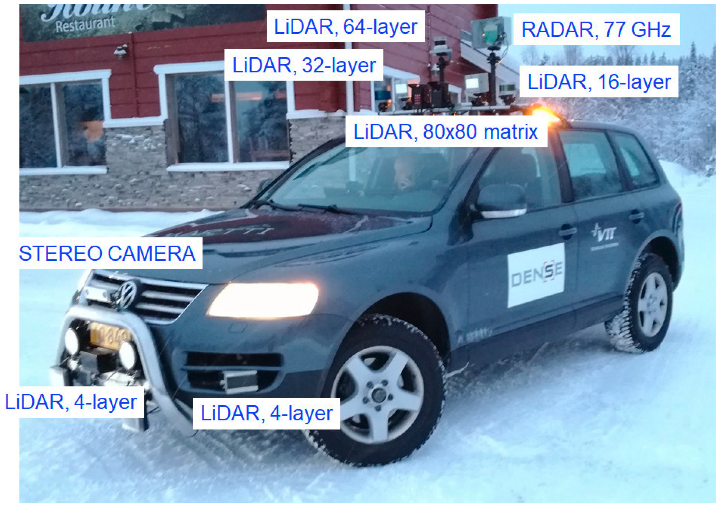
Turbulent snow tests took place outdoors in northern Finland during winter. Location and timing were chosen because of their high probability for snowy conditions. LiDARs were placed on the roof of VTT’s test vehicle Martti (Figure 2 and Figure 3) except for three Ibeo LiDARs, which were installed in the car’s bumper. Tests were performed at the airport runway in Sodankylä. There was about 20 cm of sub-zero snow on the road surface and temperature was at around −4 °C. At first, a reference drive was executed with calm conditions, i.e., no turbulent snow from a leading vehicle was present. Then, the same route was driven with another vehicle, which Martti followed as closely as possible at distances of 15–25 m in order to be surrounded by the powder snow cloud that had risen from the road’s surface. Both test drives were done for each LiDAR separately so that they would not disturb one another.
The results have been saved to the hard drives of the vehicle with GPS time-stamp and coordinates. These are used for synchronizing data between different sensor devices.
The LiDAR performance in turbulent snow and freezing conditions was visually evaluated for each sensor separately. The point cloud data are difficult to analyze with any feasible metrics since the aim is to support pattern recognition algorithms. Pattern recognition requires that there are good coverage points reflected from the surface even if there is material like snow in front of the sensor. The best method of analysis is to visually estimate whether the number of points is sufficient for estimating type and size of the object (e.g., passenger car, pedestrian, or building).
3. Results
3.1. Fog Chamber Results
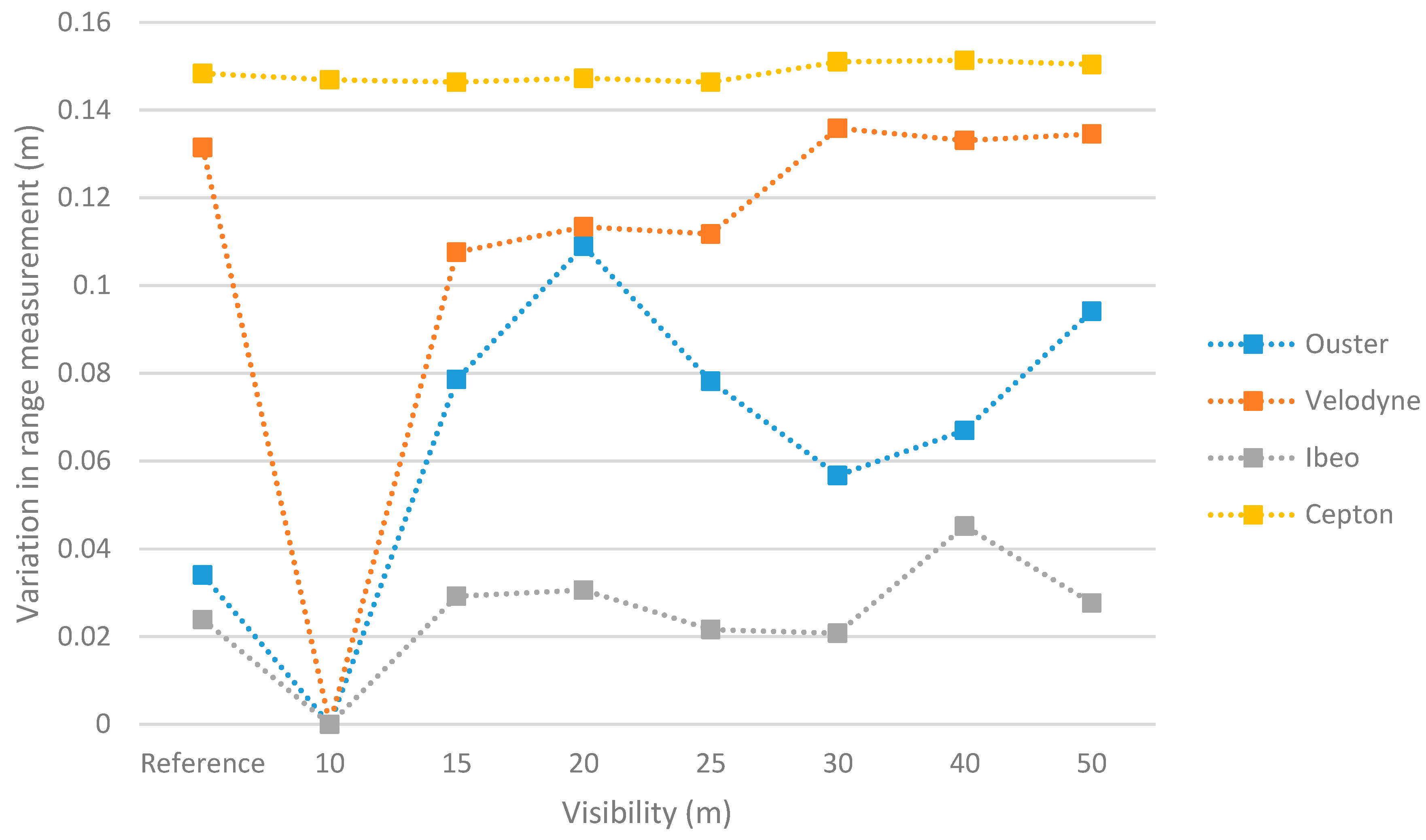
Here, variation values of range measurements for each LiDAR under different meteorological visibility conditions are presented. The aim of this test scenario is to estimate in the target area how the individual points reflected from the calibration plates varied at different fog densities. Strong variation indicates a less confident value of range measurement. Values are calculated from all the data points collected during the measuring period.
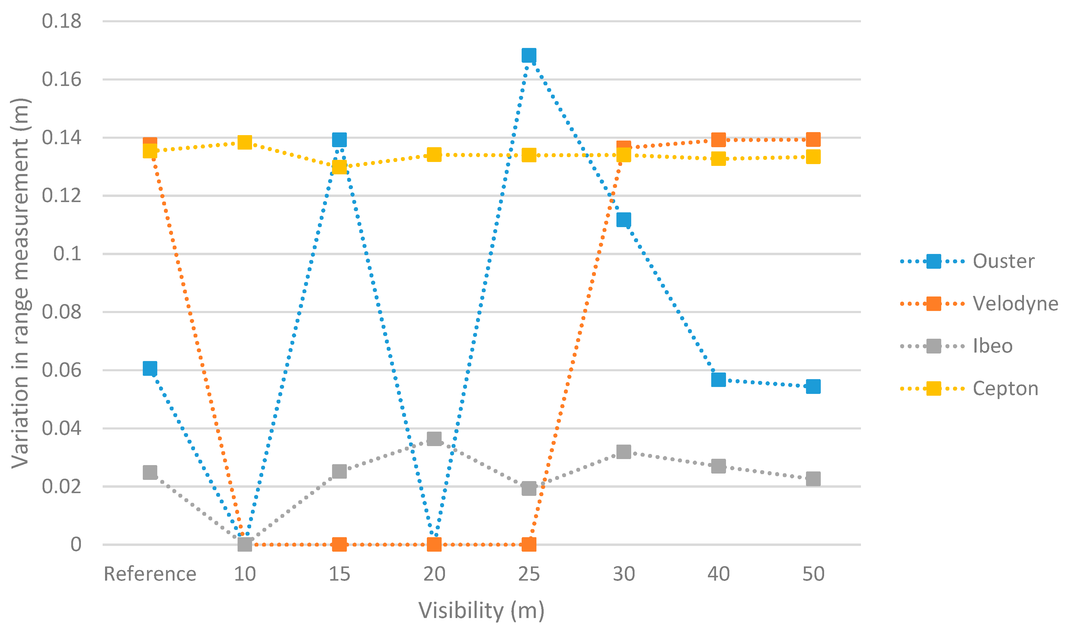
Figure 4 shows results with the target being at 10.5 m from the LiDAR setup. With meteorological visibility at 10 m, all but Cepton failed to see past the “wall” created by the dense fog. At this distance, Cepton performed constantly even though its variation value is the highest. Other tested LiDARs began detecting after the visibility increased to 15 m. After that, Velodyne and Ibeo seemed to perform steadily but Ouster’s values vary.
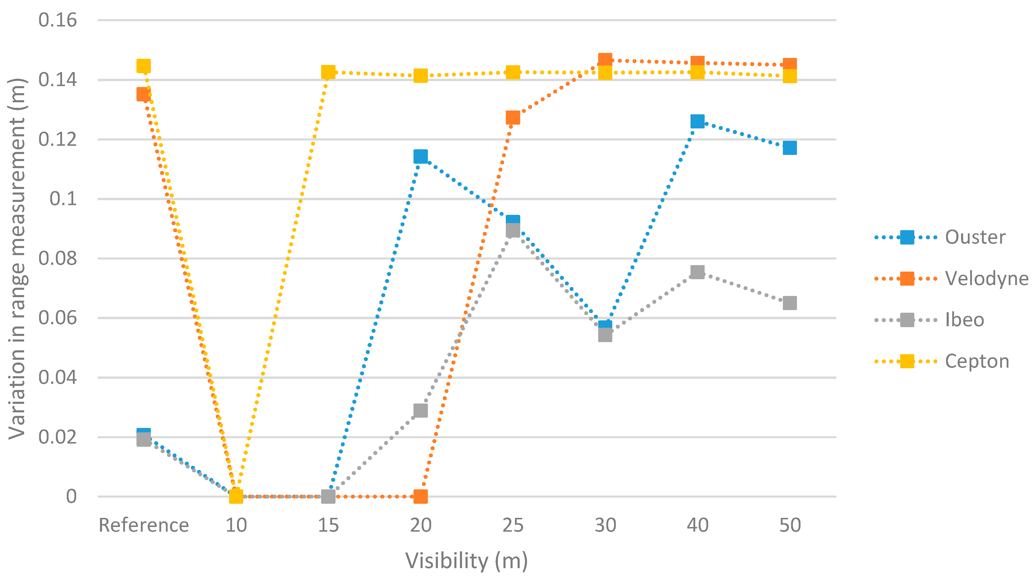
In Figure 5, the results for the 5% reflective target at a distance of 10.5 m are shown. Again, Cepton performed steadily starting from the visibility of 10 m but its variation values are higher than other sensors, excluding Velodyne. Velodyne did not detect the target until at 30 m visibility. Ibeo reached its reference level after the visibility had cleared to 15 m. Ouster had a peak at this distance, which was caused by a few outlier points in the point cloud data. Therefore, Ouster detects the black target when the visibility is increased to 25 m and even then, its variation values are significantly higher than the reference value.
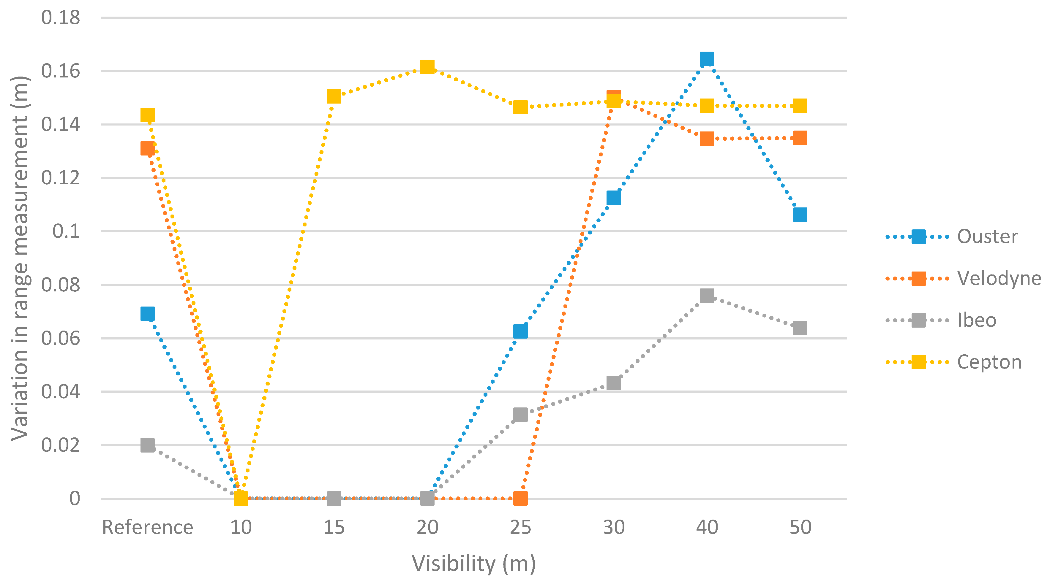
When the target was moved 5 m further away to 15.5 m from the LiDAR setup, Cepton also lost the view at first but recovered when visibility increased to 15 m. Again, Cepton’s accuracy after this was constant regarding the variation in range measurements (Figure 6). Ouster and Ibeo were able to detect the target after visibility of 20 m was reached, although their range measurement accuracy showed some variation after this and did not reach the reference level any more, even though the visibility increased. Velodyne returned to its variation level once visibility reached 25 m.
Cepton detected the 5% reflective target with the same accuracy as the 90% target (Figure 7) when visibility was more than 10 m. Ouster and Ibeo were not able to detect the target until visibility had increased to 25 m. After that, their variation values increased even though the fog cleared. Ibeo’s view may have been slightly blocked by the smaller targets, thus increasing the variation. Ouster, in general, tended to be more sensitive and gather outliers in even less dense fog. Velodyne detected the black target the first time at 30 m visibility.
In the last distance (targets 20.5 m from the sensors), the two densest visibility values (10 and 15 m) are not used in the measurements. The assumption is that none of the sensors are able to detect targets this far in such dense fog. It is also notable that for Ibeo, the reference measurement is missing.
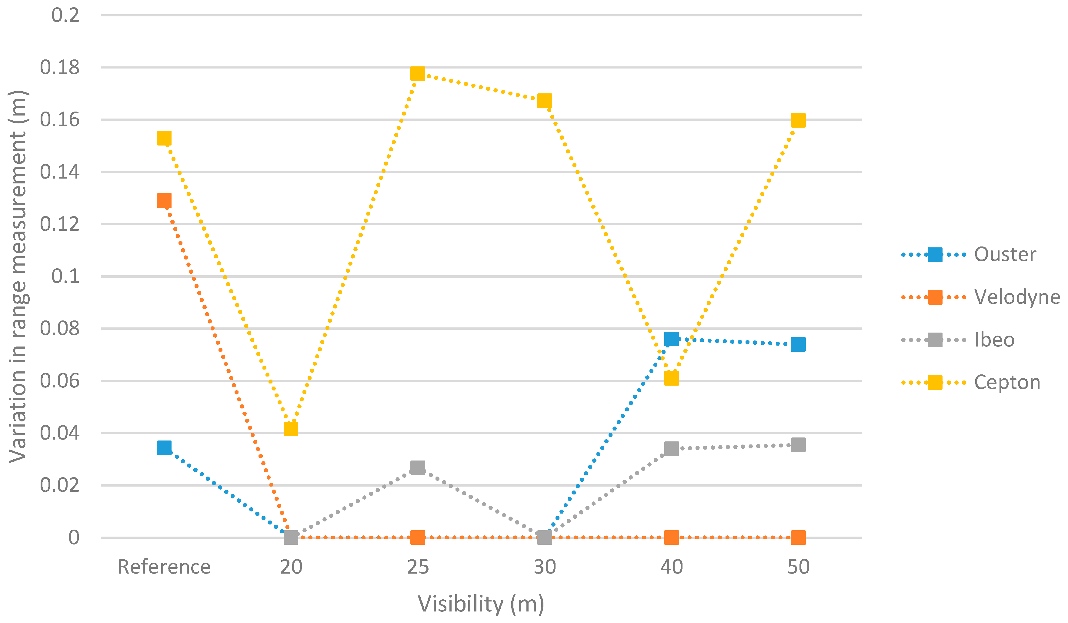
When the 90% target is located at 20.5 m, detecting it in the fog became a challenging task for all the LiDARs. However, once they did, the distance measurements were nearly as accurate as without the fog (Figure 8). Again, Cepton was the first to detect the target and returned similar variation values similar to those that it did as for the reference visibility. Both Ibeo and Ouster were able to see the target at visibility 25 m, from which their variation values increased despite the fog clearing. Velodyne detected the target at 30 m and returned to its performance level regarding the range measurement accuracy.
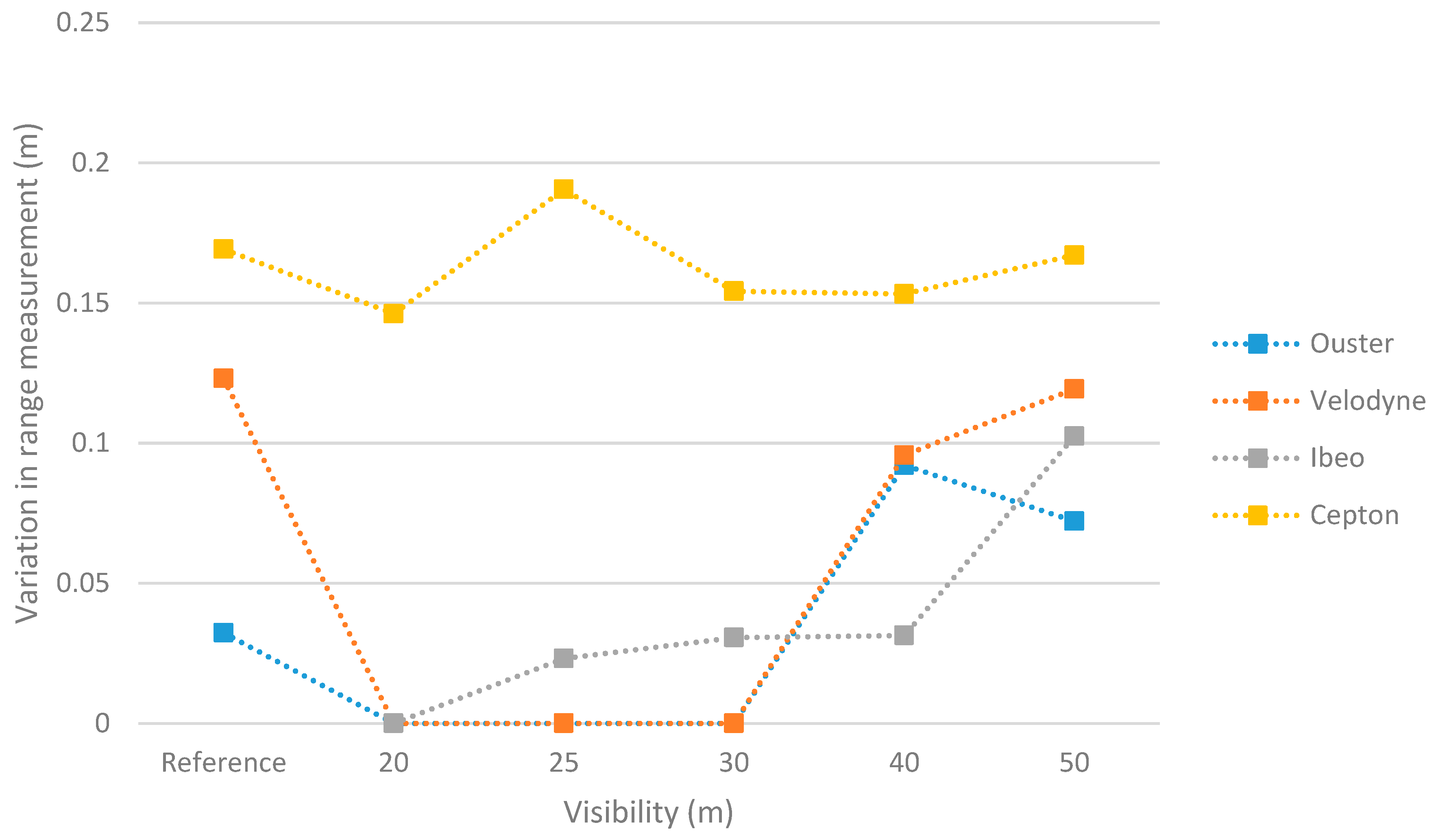
As expected, the 5% target at 20.5 m was the most difficult to detect (Figure 9). Velodyne did not see it at all, and Ouster and Ibeo saw it at visibilities larger than 30 m. Even then, Ouster’s range measurement variations were higher than the reference value. Cepton had significant drops in the variance values at 20 m and 40 m visibility. All of its measurements at this distance showed some echo points in front of the target (possibly from the smaller targets), but they were missing from the 20 m and 40 m visibility measurements.
Signal-to-noise ratio of the sensor depends not only on atmospheric influence but also on other attributes like filtering the signal. Filtering is normally very sensor supplier-specific and depends on the number of echoes that LiDAR reads. In case of multi-echo, SNR is normally less since the receiver captures also weak signals causing more noise.
3.2. Turbulent Snow Test Results
The results are presented with a cumulative intensity image of 25 scans from each LiDARs test run together with the leading vehicle. All presented LiDARs were installed leaning a tad forward. Hence, the density of layers is higher in front of the test vehicle. This install was chosen because we wanted to have more layers hitting the road surface and, thus, more accuracy in that area. Cepton and Ibeo data are omitted in this inspection. Because of Ibeo’s location in the bumper, it was not possible to obtain a comparable point cloud. Cepton was malfunctioning in the tests and produced only noisy and illogical point clouds. Thus, its results were considered useless.
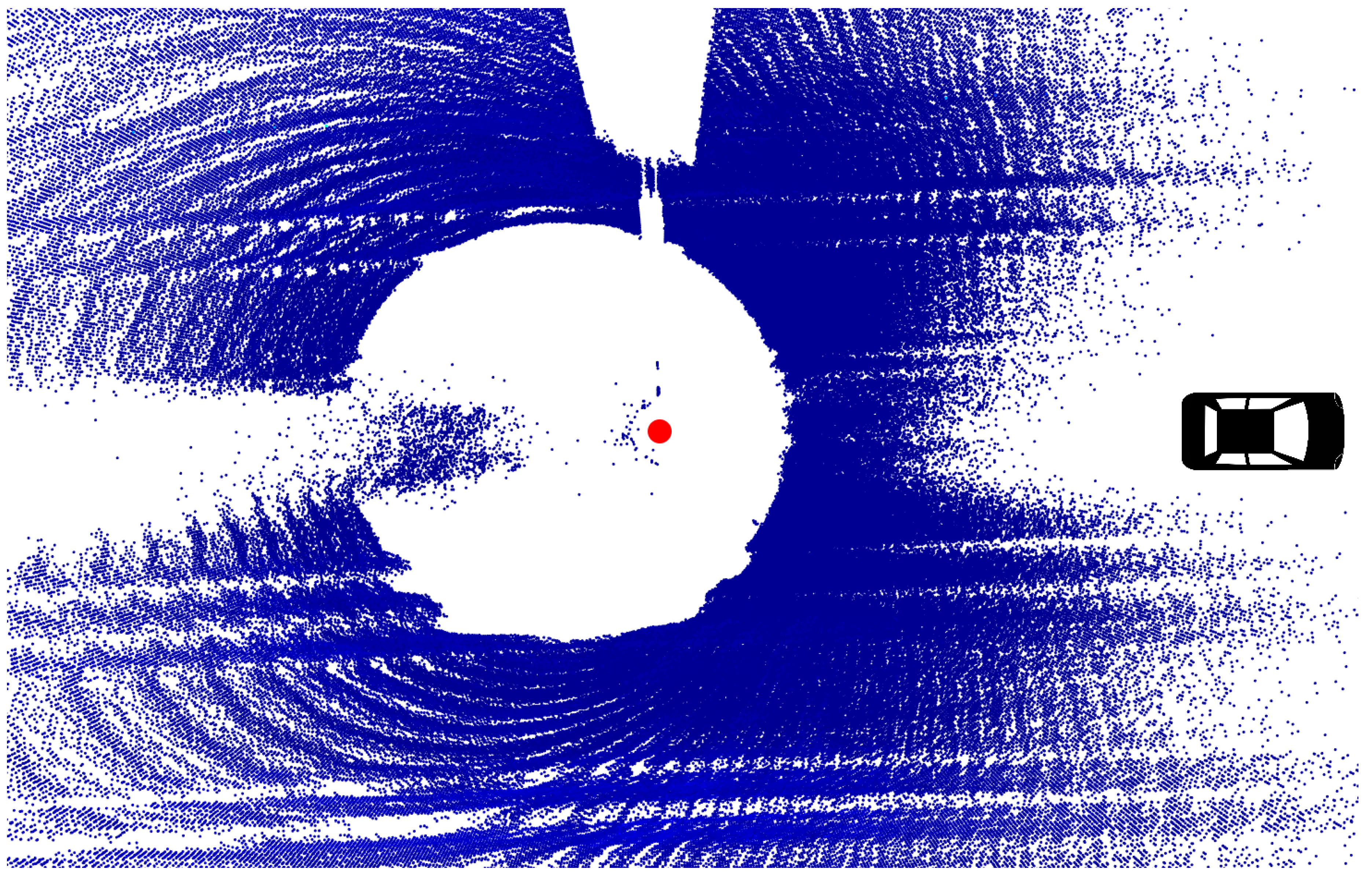
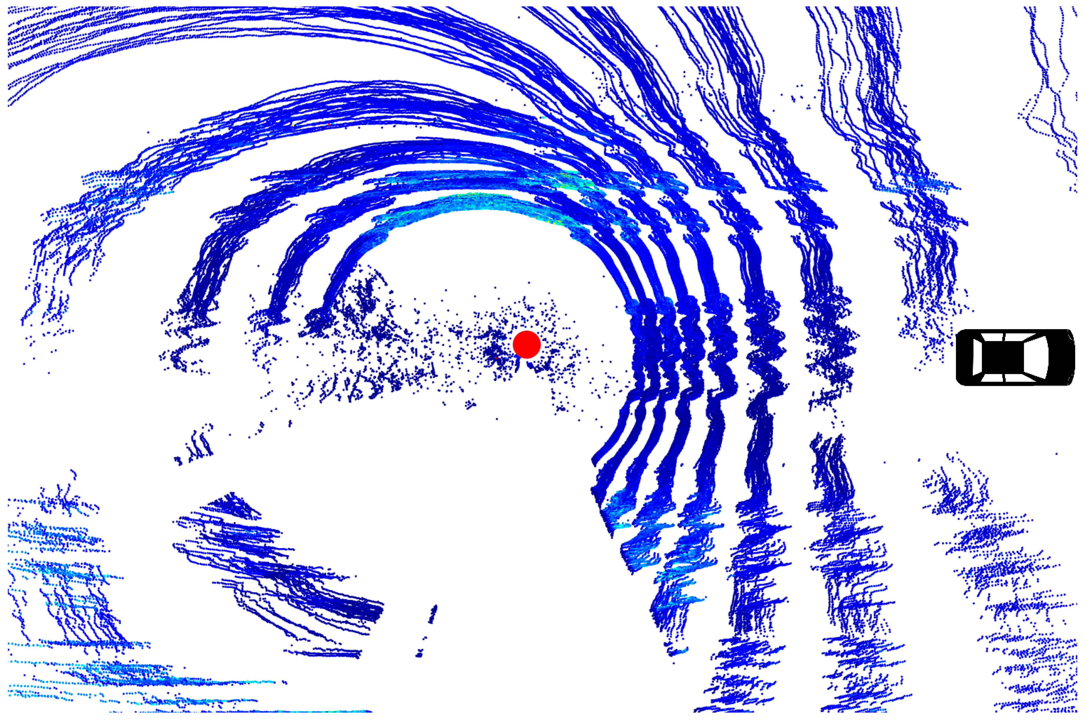
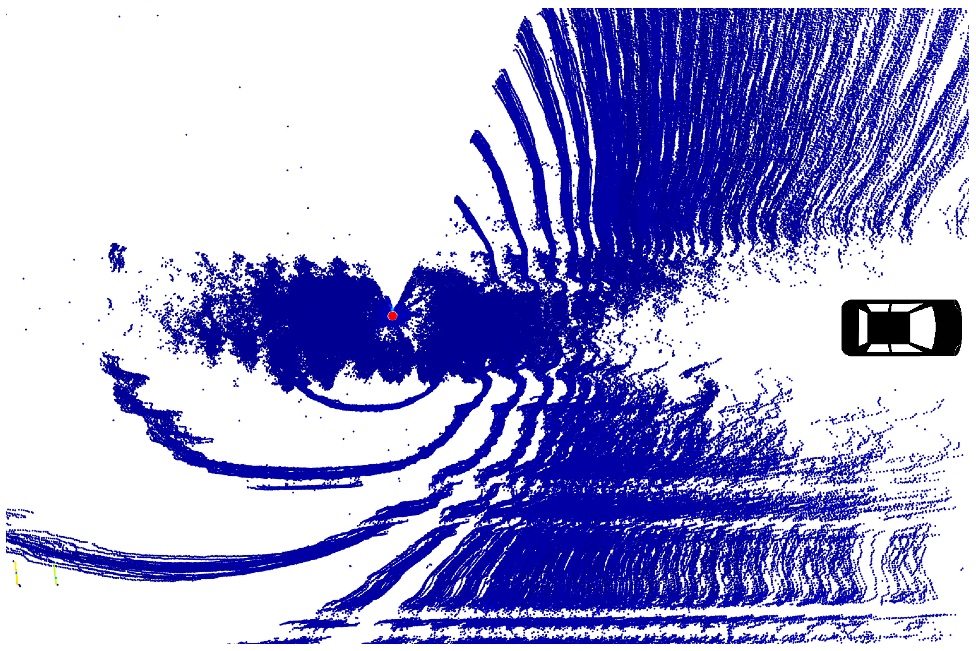
In all the images, there are constant empty regions (the upper part of the image in Ouster and Robosense, the lower part in Velodyne), which are caused by another sensor located next to the tested one (see Figure 3 for a detailed image of installation). The sensor is marked with a red dot and the driving direction is to the right in all the images. The leading vehicle is visualized in the images in its approximate location.
In Ouster readings (Figure 10), the powder snow blocks the view both in front of and behind Martti. These appear as empty regions in the point cloud scans. The leading vehicle produces the cloud in the frontal area and Martti itself causes the cloud behind. The snow dust itself is not visible in the data, although some points do appear behind the sensor. The distance from the sensor to the first layer is 4.4 m in the front and 11.5 m in the back.
Figure 11 shows typical readings for Velodyne when it is following another vehicle in snow. Again, the powder snow itself is not detected (except for a few points around the sensor) but the view forward and back are missing because of the turbulent snow produced by the leading vehicle and Martti. The distance from the sensor to the first layer is 4.6 m in the front and 8.9 m in the back.
Robosense readings in Figure 12 differ from the other two sensors. Here, the view of the front and back are again empty of echo points but the snow is seen as a dense cloud surrounding the sensor, too. The effect is similar to the readings produced by the fog with other tested sensors. The diameter of the first layer from the front to the back view is 7.7 m.
4. Discussion
In conclusion, all tested LiDARs performed worse in fog and turbulent snow than in clear weather conditions, as expected. In fog chamber tests, every sensor’s performance decreased the denser the fog and the further the target. Making a direct comparison, Cepton’s different approach proved the most efficient in stationary fog chamber tests but its point clouds are quite noisy. No significant differences were found between the other sensors. The darker target was more difficult for the sensors to detect than the lighter one.
In the turbulent snow tests, all tested sensors were blocked by the powder snow and their viewing distance was shortened. However, from these tests, it is not possible to say if some sensor performed absolutely better than the others did. The powder snow itself was not visible in two of the sensors’ data, but its presence was observable by the missing echo points in front of and behind the test vehicle. Only Robosense produced points that directly showed the presence of snow. It is notable that not only does the leading vehicle cause the snow to whirl, but the test vehicle itself does as well. This makes detection in that direction difficult as well and shortens the viewing distance. Temperatures that were a few degrees centigrade below zero did not affect the performance of the LiDARs. However, based on these tests we cannot say how well they would perform in even colder environment.
There are no ideal fog, rain, or snow conditions that create a single threshold when the objects are not visible anymore. Moreover, this is highly dependent on LiDAR type. For example, with multilayer LiDAR (e.g., 16 or 32), the influence of one single laser spot is less significant. However, in the future, the aim is to investigate if the parameters and reliability levels of object recognition can be more precisely adapted according to density of the atmospheric changes. This would be essential, especially when considering sensor data fusion and having an understanding which sensor data the automated vehicle should rely on. At this level of LiDAR performance, fully autonomous vehicles that rely on accurate and reliable sensor data cannot be guaranteed to work in all conditions and environments. The powder snow on the roads is very common in colder environments for much of the year and, thus, is not ignorable. The cold temperatures may also bring other difficulties to the used sensors that are, as yet, unknown to us. This provides encouragement for the continued investigation of the LiDAR performance in these challenging conditions.
Author Contributions
M.J. is primarily responsible for planning the test scenarios and executing the analysis of range degradation in various weather conditions. In addition, she was also in charge of detailed analysis and reporting the key findings. M.K. contributed to the article by identifying the automated driving requirements in various weather conditions. He planned the test scenarios and analyzed the pros and cons of the various automotive LiDARs. P.P. has been the main software developer for programming analysis tools and gathering data in various weather conditions. He has also been in charge of analysis of the data.
Funding
This research was funded by the DENSE-EU-ECSEL project (Grant Agreement ID: 692449). DENSE is a joint European project which is sponsored by the European Commission under a joint undertaking. The project was also supported by Business Finland and other national funding agencies in Europe.
Acknowledgments
We would like to thank the DENSE-EU-ECSEL project and the Forum for Intelligent Machines (FIMA) for collaboration in both fog and snow tests and the opportunity to use obtained data for this study.
Conflicts of Interest
The authors declare no conflict of interest. The funders had no role in the design of the study; nor in the collection, analyses, or interpretation of data; nor in the writing of the manuscript or in the decision to publish the results.
References
- Rasshofer, R.H.; Spies, M.; Spies, H. Influences of weather phenomena on automotive laser radar systems. Adv. Radio Sci. 2011, 9, 49–60. [Google Scholar] [CrossRef] [Green Version]
- Hasirlioglu, S.; Doric, I.; Lauerer, C.; Brandmeier, T. Modeling and simulation of rain for the test of automotive sensor systems. In Proceedings of the 2016 IEEE Intelligent Vehicles Symposium (IV); IEEE: Gotenburg, Sweden, 2016; pp. 286–291. [Google Scholar]
- Fersch, T.; Buhmann, A.; Koelpin, A.; Weigel, R. The influence of rain on small aperture LiDAR sensors. In Proceedings of the 2016 German Microwave Conference (GeMiC); IEEE: Bochum, Germany, 2016; pp. 84–87. [Google Scholar]
- Reway, F.; Huber, W.; Ribeiro, E.P. Test Methodology for Vision-Based ADAS Algorithms with an Automotive Camera-in-the-Loop. In Proceedings of the 2018 IEEE International Conference on Vehicular Electronics and Safety (ICVES); IEEE: Madrid, Spain, 2018; pp. 1–7. [Google Scholar]
- Goodin, C.; Carruth, D.; Doude, M.; Hudson, C. Predicting the Influence of Rain on LIDAR in ADAS. Electronics 2019, 8, 89. [Google Scholar] [CrossRef]
- Bijelic, M.; Gruber, T.; Ritter, W. A Benchmark for Lidar Sensors in Fog: Is Detection Breaking Down? In Proceedings of the 2018 IEEE Intelligent Vehicles Symposium (IV); IEEE: Changshu, China, 2018; pp. 760–767. [Google Scholar] [Green Version]
- Hasirlioglu, S.; Kamann, A.; Doric, I.; Brandmeier, T. Test methodology for rain influence on automotive surround sensors. In Proceedings of the 2016 IEEE 19th International Conference on Intelligent Transportation Systems (ITSC); IEEE: Rio de Janeiro, Brazil, 2016; pp. 2242–2247. [Google Scholar]
- Hasirlioglu, S.; Doric, I.; Kamann, A.; Riener, A. Reproducible Fog Simulation for Testing Automotive Surround Sensors. In Proceedings of the 2017 IEEE 85th Vehicular Technology Conference (VTC Spring); IEEE: Sydney, Australia, 2017; pp. 1–7. [Google Scholar]
- Kim, B.K.; Sumi, Y. Performance evaluation of safety sensors in the indoor fog chamber. In Proceedings of the 2017 IEEE Underwater Technology (UT); IEEE: Busan, Korea, 2017; pp. 1–3. [Google Scholar]
- Daniel, L.; Phippen, D.; Hoare, E.; Stove, A.; Cherniakov, M.; Gashinova, M. Low-THz Radar, Lidar and Optical Imaging through Artificially Generated Fog. In Proceedings of the International Conference on Radar Systems (Radar 2017); Institution of Engineering and Technology: Belfast, UK, 2017. [Google Scholar]
- Kutila, M.; Pyykonen, P.; Holzhuter, H.; Colomb, M.; Duthon, P. Automotive LiDAR performance verification in fog and rain. In Proceedings of the 2018 21st International Conference on Intelligent Transportation Systems (ITSC); IEEE: Maui, HI, USA, 2018; pp. 1695–1701. [Google Scholar]
- Filgueira, A.; González-Jorge, H.; Lagüela, S.; Díaz-Vilariño, L.; Arias, P. Quantifying the influence of rain in LiDAR performance. Measurement 2017, 95, 143–148. [Google Scholar] [CrossRef]
- Colomb, M.; Hirech, K.; André, P.; Boreux, J.J.; Lacôte, P.; Dufour, J. An innovative artificial fog production device improved in the European project “FOG.”. Atmos. Res. 2008, 87, 242–251. [Google Scholar] [CrossRef]
Figure 1.
LiDAR setup in Clermont-Ferrand fog chamber.

Figure 2.
Sensor installation in the Martti test vehicle.

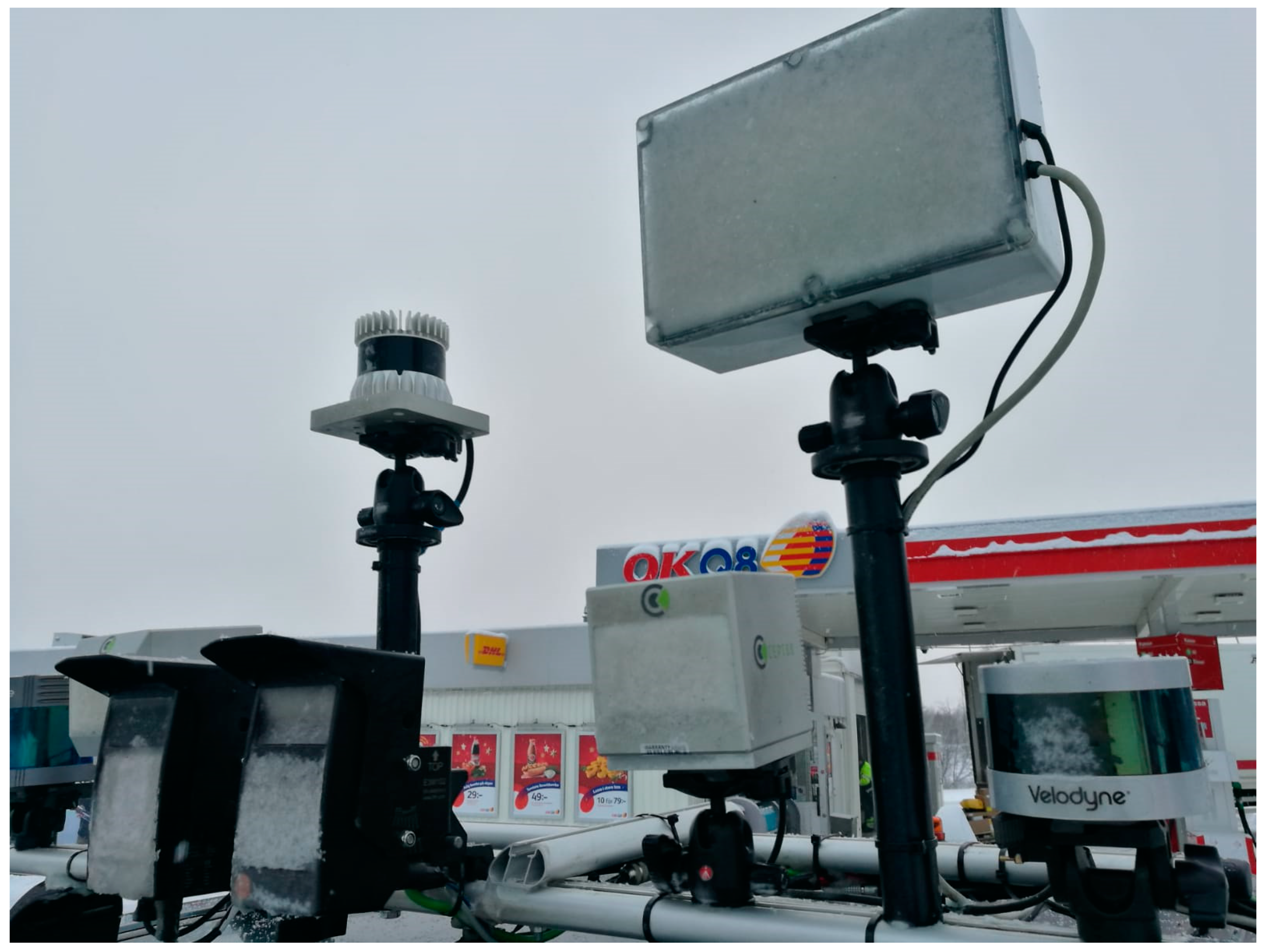
Figure 3.
Frozen sensors when the temperature is less than −15 °C.

Figure 4.
Standard deviation of range values from echo points reflected from the 90% target located at 10 m.
Figure 4.
Standard deviation of range values from echo points reflected from the 90% target located at 10 m.

Figure 5.
Standard deviation of range values from echo points reflected from the 5% target located at 10 m.
Figure 5.
Standard deviation of range values from echo points reflected from the 5% target located at 10 m.

Figure 6.
Standard deviation of range values from echo points reflected from the 90% target located at 15 m.
Figure 6.
Standard deviation of range values from echo points reflected from the 90% target located at 15 m.

Figure 7.
Standard deviation of range values from echo points reflected from the 5% target located at 15 m.
Figure 7.
Standard deviation of range values from echo points reflected from the 5% target located at 15 m.

Figure 8.
Standard deviation of range values from echo points reflected from the 90% target located at 20 m.
Figure 8.
Standard deviation of range values from echo points reflected from the 90% target located at 20 m.

Figure 9.
Standard deviation of range values from echo points reflected from the 5% target located at 20 m.
Figure 9.
Standard deviation of range values from echo points reflected from the 5% target located at 20 m.

Figure 10.
An Ouster point cloud when driving behind a leading vehicle.

Figure 11.
A Velodyne point cloud when driving behind a leading vehicle.

Figure 12.
A Robosense point cloud when driving behind a leading vehicle.


Table 1.
Specifications of the tested light detection and ranging sensors (LiDARs).
| Specifications | ibeo Lux | Velodyne VLP-16 | Ouster OS-164 | Robosense RS-LiDAR-32 | Cepton HR80T/W |
|---|---|---|---|---|---|
| Layers | 4 | 16 | 64 | 32 | no (80 × 80 points, 160 × 64 points) |
| Vertical FOV | 3.2° | 30° (+15°~−15°) | 31.6° (+15.8°~−15.8°) | 40° (+15°~−25°) | horizontal and vertical FOV: 15° × 15°, 60° × 24° |
| Vertical resolution | 0.8° | 2.0° | 0.5° | 0.33°~4.66° | 15°/80 points = 0.19°, 60°/160 points = 0.38° |
| Horizontal resolution | 0.125°, 0.25°, or 0.5° (110°) | 0.1°, 0.2°, or 0.4° (360°) | 0.175° and 0.35° (360°) | 0.09°, 0.18°, or 0.36° (360°) | 0.19°, 24°/64 points = 0.38° |
| Scans per second | 12.5, 25, or 50 Hz | 5, 10, or 20 Hz | 10 or 20 Hz | 5, 10, or 20 Hz | 10 Hz |
| Range @ reflectivity | 90 m @ 90%, 30 m @ 10% | 100 m @ ?% | 40 m @ 10%, 120 m @ 80% | 200 m @ 20% | 200 m @ ?, 100 m @ ? |
| Distance accuracy | 4 cm | ±3 cm | 1.2 cm | ±5 cm (typical) | 2.5 cm |
| No. of returns / point | 3 | 2 | 1 | 1 | 1 |
| Intensity measured | yes | yes | yes | yes | yes |
| Operating temperature | −40~+86 °C | −10~+60 °C | −20~+50 °C | −10~+60 °C | −20~+65 °C |
| IP | 69 K | 67 | 67 | 68 | 67 |
| Wavelength | 905 nm | 903 nm | 850 nm | 905 nm | 905 nm |
© 2019 by the authors. Licensee MDPI, Basel, Switzerland. This article is an open access article distributed under the terms and conditions of the Creative Commons Attribution (CC BY) license (http://creativecommons.org/licenses/by/4.0/).
Share and Cite
MDPI and ACS Style
Jokela, M.; Kutila, M.; Pyykönen, P. Testing and Validation of Automotive Point-Cloud Sensors in Adverse Weather Conditions. Appl. Sci. 2019, 9, 2341. https://0-doi-org.brum.beds.ac.uk/10.3390/app9112341
AMA Style
Jokela M, Kutila M, Pyykönen P. Testing and Validation of Automotive Point-Cloud Sensors in Adverse Weather Conditions. Applied Sciences. 2019; 9(11):2341. https://0-doi-org.brum.beds.ac.uk/10.3390/app9112341
Chicago/Turabian StyleJokela, Maria, Matti Kutila, and Pasi Pyykönen. 2019. "Testing and Validation of Automotive Point-Cloud Sensors in Adverse Weather Conditions" Applied Sciences 9, no. 11: 2341. https://0-doi-org.brum.beds.ac.uk/10.3390/app9112341
Note that from the first issue of 2016, this journal uses article numbers instead of page numbers. See further details here.