A Comparative Study of PSO-ANN, GA-ANN, ICA-ANN, and ABC-ANN in Estimating the Heating Load of Buildings’ Energy Efficiency for Smart City Planning

Abstract

Energy-efficiency is one of the critical issues in smart cities. It is an essential basis for optimizing smart cities planning. This study proposed four new artificial intelligence (AI) techniques for forecasting the heating load of buildings’ energy efficiency based on the potential of artificial neural network (ANN) and meta-heuristics algorithms, including artificial bee colony (ABC) optimization, particle swarm optimization (PSO), imperialist competitive algorithm (ICA), and genetic algorithm (GA). They were abbreviated as ABC-ANN, PSO-ANN, ICA-ANN, and GA-ANN models; 837 buildings were considered and analyzed based on the influential parameters, such as glazing area distribution (GLAD), glazing area (GLA), orientation (O), overall height (OH), roof area (RA), wall area (WA), surface area (SA), relative compactness (RC), for estimating heating load (HL). Three statistical criteria, such as root-mean-squared error (RMSE), coefficient determination (R²), and mean absolute error (MAE), were used to assess the potential of the aforementioned models. The results indicated that the GA-ANN model provided the highest performance in estimating the heating load of buildings’ energy efficiency, with an RMSE of 1.625, R² of 0.980, and MAE of 0.798. The remaining models (i.e., PSO-ANN, ICA-ANN, ABC-ANN) yielded lower performance with RMSE of 1.932, 1.982, 1.878; R² of 0.972, 0.970, 0.973; MAE of 1.027, 0.980, 0.957, respectively.

1. Introduction

One of the indispensable components for smart cities is energy and the applications of artificial intelligence (AI) [1]. Nowadays, smart cities are becoming more popular and the first choice for those who want a comfortable and productive life [2,3,4,5]. This includes intelligent, modern, energy efficient utilities, as well as sustainable environmental protection [6,7,8]. Of those components, heating load (HL) and cooling load (CL) systems are a part of energy efficiency. Many studies were conducted to predict and optimize the use of buildings’ energy efficiency (EEB) as well as building energy consumption [9]. For instance, Catalina et al. [10] used multiple regression method to estimate the demand for heating energy of the building. The south equivalent surface, global heat loss coefficient of building, and the difference between the sol-air and the indoor temperatures, were used as the input variables to estimate the demand of heating energy in their study. Their positive results were confirmed with a determination coefficient (R²) of 0.987. Chou, Bui [11] also developed an ensemble model based on support vector regression (SVR) and an artificial neural network (ANN) to predict HL and CL for building design, called ANN-SVR, using the datasets of 17 buildings. A variety of the other models were also considered and developed to investigate and compare with their proposed ANN-SVR model, including SVR, ANN, chi-squared automatic interaction detector, classification and regression tree, and general linear regression. Their results confirmed the feasibility of AI techniques designing and optimizing EEB systems, especially the ANN-SVR model with a mean absolute percentage error (MAPE) below 4% and root-mean-squared error (RMSE) lower than 39%–65.9% in a comparison of the previous works [12,13]. In another study, Castelli et al. [14] applied a genetic programming (GP) model for evaluating the energy efficiency of EEB systems. Three forms of GP were investigated and compared, such as geometric sematic GP (GSGP), GSGP with local search (HYBRID), and HYBRID with linear scaling (HYBRID-LIN). Their results indicated that the HYBRID-LIN technique provided better results than the other techniques (i.e., GP, HYBRID). Deep learning techniques in AI have also been developed to estimate the energy efficiency of EEB systems (i.e., CL) by Fan et al. [15]. The potential of deep learning was exploited and interpreted for a variety of AI models in predicting CL of EEB systems during 24 h, including multiple linear regression (MLR), elastic net, random forest (RF), gradient boosting trees (GBT), SVR, extreme gradient boosting (XGB), and deep learning (DNN). Their results showed that their XGB model with deep learning technique yielded the highest accuracy with an RMSE of 106.5 and MAE of 71.6. The efforts for optimizing an ANN model using uncertainty means and sensitivity analyses were conducted to predict the energy demand of buildings by Ascione et al. [16]. Its performance was proven in a short-term prediction of the energy demand of buildings. As a result, their findings showed the powerful potential of the optimized ANN model in predicting the energy demand of buildings with an R² of 0.995, and the average relative error is between 2.0% and 11%. Ngo [17] also developed an ensemble machine learning model to predict the CL of EEB systems with high accuracy (e.g., RMSE = 158.77, MAE = 112.07, MAPE = 6.17%, and R² = 0.990). By the use of a hybrid model (M5Rules-particle swarm optimization (PSO)), Nguyen et al. [18] predicted the CL of EEB systems with a promising result. A similar study for predicting the HL of EEB systems was also performed by Bui et al. [19], using a novel hybrid approach, i.e., M5Rules-genetic algorithm (GA). By the use of the meta-heuristic algorithms (i.e., PSO, GA) to optimize the M5Rules model, Nguyen et al. [18] and Bui et al. [19] provided two new hybrid intelligent techniques (i.e., M5Rules-PSO and M5Rules-GA) to predict the CL and HL of EEB systems with high accuracy, i.e., RMSE of 0.0066, 0.0548, and R² of 0.999, 0.998, for the M5Rules-PSO and M5Rules-GA, respectively. Additionally, many other studies used/applied/developed AI techniques for evaluating and predicting energy consumption as well as its efficiency [20,21,22,23,24].

According to the best review of the authors, meta-heuristics algorithms with a combination of ANN model was considered and developed in many areas with high reliability [25,26,27,28,29,30,31,32,33,34,35]; however, they are not still considered and prepared for estimating the HL of EEB systems. Therefore, this study developed and proposed four novel hybrid models based on four meta-heuristics algorithms and ANN model, for estimating the HL of EEB systems, namely PSO-ANN, GA-ANN, imperialist competitive algorithm (ICA)-ANN, and artificial bee colony (ABC)-ANN models. Four meta-heuristics algorithms were considered in this study, including artificial bee colony (ABC) optimization, particle swarm optimization (PSO), imperialist competitive algorithm (ICA), and genetic algorithm (GA). They were abbreviated as ABC-ANN, PSO-ANN, ICA-ANN, and GA-ANN models.

2. Data Collection and Its Characteristics

For data collection, twelve types of buildings were investigated and simulated by Ecotect computer software [13]. Accordingly, 768 experimental datasets were simulated and collected by Tsanas, Xifara [13]. To ensure the diverse of the dataset, 69 other buildings (during the winter of 2018) were also considered and investigated in Vietnam with similar conditions and materials. Finally, a total of 837 experimental datasets were considered and analyzed for estimating the HL of EEB systems in this work. Floor/surface area (SA), roof area (RA), wall area (WA), and overall height (OH), were considered as the main components of the buildings, as illustrated in Figure 1. Additionally, glazing area distribution (GLAD), relative compactness (RC), glazing area (GLA), and orientation (O) were also extended investigated for estimating the HL of EEB systems.

Table 1. Summary of the heating load of the energy efficiency database used.

Elements	GLAD	GLA	O	OH	RA
Min.	1.000	0.00	1.000	1.040	138.2
Mean	3.016	22.54	2.581	5.509	180.5
Max.	5.000	50.00	4.000	8.479	223.2
Elements	WA	SA	RC	HL	-
Min.	234.2	488.6	0.4194	5.353	-
Mean	350.7	659.4	0.7954	29.575	-
Max.	459.7	825.0	1.1960	65.034	-

Note: glazing area distribution (GLAD), glazing area (GLA), orientation (O), overall height (OH), roof area (RA), wall area (WA), surface area (SA), relative compactness (RC), heating load (HL).

summaries the heating load of the energy efficiency database used herein. Also, Figure 2 illustrates the properties of the dataset used for estimating the HL of EEB systems in this study.

3. Methods

3.1. Particle Swarm Optimization (PSO) Algorithm

PSO is a swarm algorithm inspired by the behavior of the particles/social animals, such as fish, or birds. It was introduced and developed by Eberhart, Kennedy [36] and classified as one of the metaheuristic techniques. It was considered as an evolutionary computation technique in the statistical community with many advantages [29,37,38,39]. This method attempts to take a strong point of the information-sharing procedure from the cluster that affects the overall swarm behavior. Thus, PSO works with the potential solution of a population rather than a single separate item. The best solution is found out based on the experiences of all individuals in the swarm during searching. The PSO algorithm implements six steps for optimal searching as the following pseudo-code [40]:

Algorithm: The particle swarm optimization (PSO) pseudo-code for the optimization process
1	for each particle i
2	for each dimention d
3	Initialize position xid randomly within permissible range
4	Initialize velocity vid randomly within permissible range
5	end for
6	end for
7	Iteration k = 1
8	do
9	for each particle i
10	Calculate fitness value
11	if the fitness value is better than p_bestid in history
12	Set current fitness value as the p_bestid
13	end if
14	end for
15	Choose the particle having the best fitness value as the g_bestid
16	for each particle i
17	for each dimention d
18	Calculate velocity according to the following equation $v_j^{i+1}=w{v}_j^{(i)}+(c_1\times r_1\times (localbes{t}_j-x_j^{(i)}))+(c_2\times r_2\times (\mathrm{global}bes{t}_j-x_j^{(i)})),v_{\min }\le v_j^{(i)}\le v_{\max }$
19	Update particle position according to the following equation $x_j^{i+1}=x_j^{(i)}+v_j^{(i+1)};j=1,2,\dots ,n$
20	end for
21	end for
22	k = k+1
23	while maximum iterations or minimum error criteria are not attained

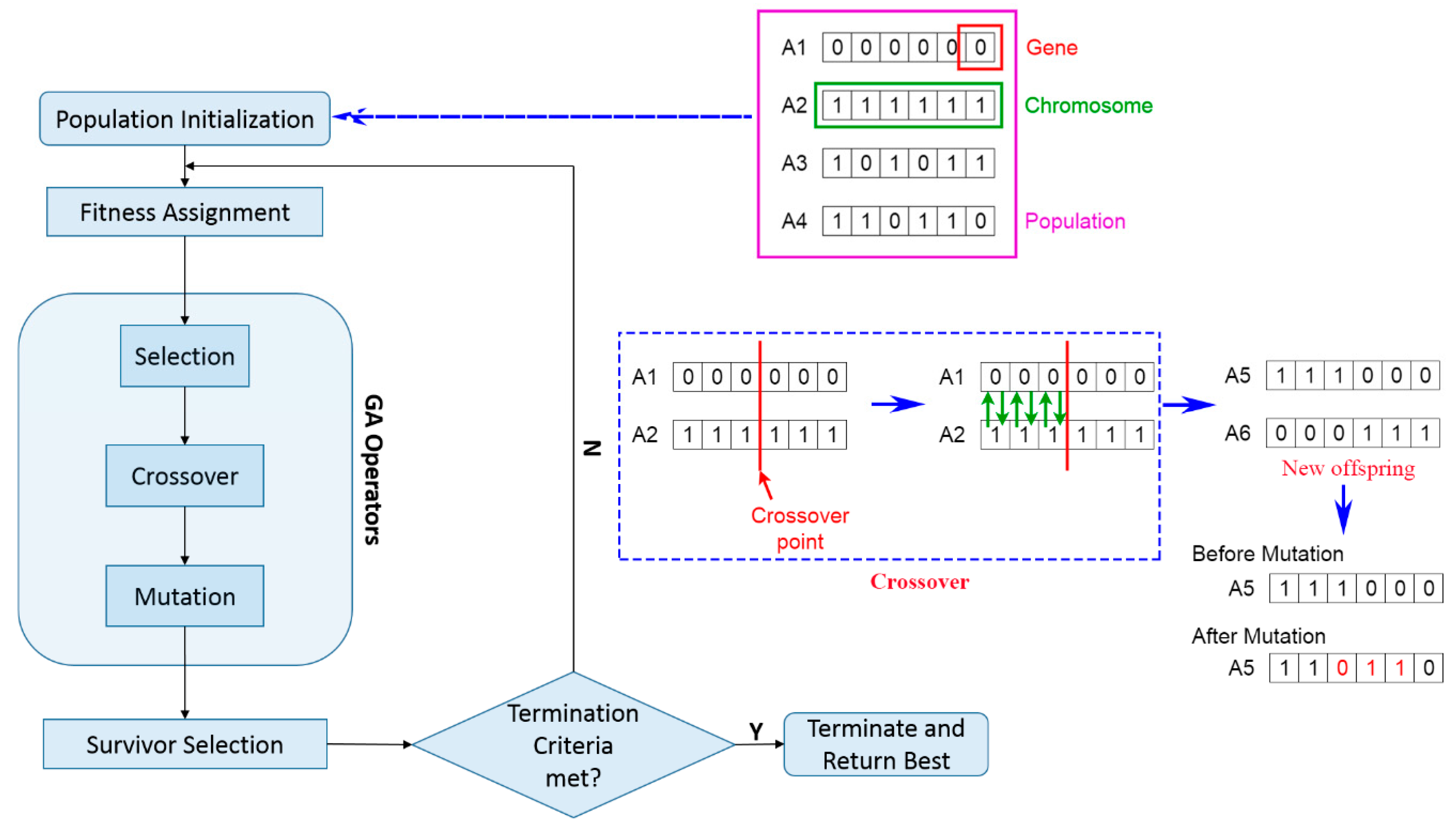
3.2. Genetic Algorithm (GA)

Genetic algorithm (GA) is an optimization algorithm based on Darwin’s theory of natural selection to find the optimal values of a function [41,42]. GA represents one branch of evolutionary computation [43]. It applies the principles: genetics, mutation, natural selection, and crossover. A set of initial candidates is created, and their corresponding fitness values are calculated [44,45,46]. In GA, many processes are random, like in evolution. However, this optimization technique allows setting random levels and levels of control. In this way, GA is considered as a robust and comprehensive search algorithm. The executable GA may be specified as following (Figure 3):

• Population origination: randomly generates a population of n individuals.
• Calculate the adaptive values: Estimating the adaptation of each individual.
• Stop condition: check the state to finish the algorithm.
• Selection: select two parents from the old population according to their adaptation (the higher the individual is, the more likely they are to be selected).
• Crossover: with each probability selected, a crossover between two parents is made to create a new individual.
• Mutation: for each potential variation selected, new individuals are formed.
• Select the result: if the stopping condition is satisfied, the algorithm ends, and the best solution is found in the current population. When the stopping conditions are not met, the new society will be continually created by repeating three steps: selection, crossover, and mutation.

GA has two necessary stopping conditions:

• Based on the chromosome structure, controlling the number of genes that are converging, if the number of genes is united at a point or beyond that point, the algorithm ends.
• Based on the special meaning of the chromosome, examine the change of the algorithm after each generation. If the difference is less than a constant, then the algorithm ends.

3.3. Imperialist Competitive Algorithm (ICA)

Inspired by the simulation of a computer of human social evolution, the ICA was proposed by Atashpaz-Gargari, Lucas [47] to solve optimization problems. It is one of the swarm intelligence techniques that can effectively solve continuous functions [48,49,50]. Briefly, ICA is a global search algorithm inspired by imperialistic competition and based on a social policy of imperialism. Accordingly, the most potent empire will dominate many colonies and their sources of use. If an empire collapses, other realms will compete for the territory. The core of the ICA can be described by the following steps:

• Create random search spaces and initial empires;
• Assimilation of colonies: the colonies moved in different directions to the realms;
• Revolution: random changes occur in the characteristics of each country;
• Exchange the position of the territory for the empire. A colony with a better place than the realm will have the opportunity to rise and control the empire, replacing the existing empire;
• Imperial competition: competition and conquest occurs among the empires to possess each other’s colonies;
• Eliminate weaker empires. Natural selection rules are applied. Weak empires will collapse and lose the entire colonies;
• If the stop condition is satisfied, stop, otherwise return to step 2;
• End.

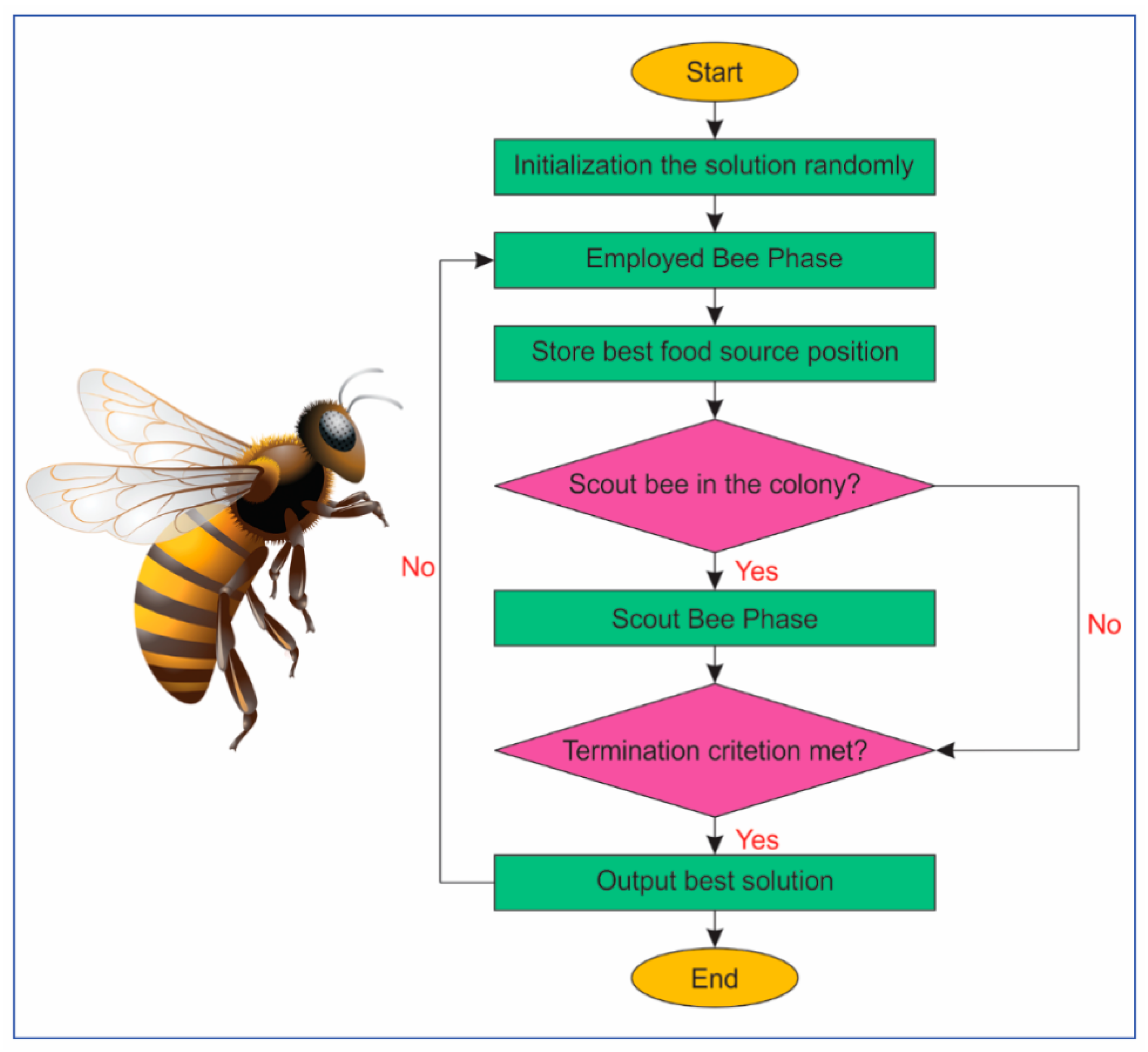
3.4. Artificial Bee Colony (ABC)

Optimization algorithms are one of the branches of AI which have been researched and developed based on nature’s inspiration, and swarm intelligence is one of them. Inspired by the bees’ search for food, Karaboga [51] introduced the ABC optimization algorithm as a robust tool for optimization problems. Although it is pure swarm intelligence, valid for both discrete optimization problems and continuous are significant [52,53,54]. In the ABC algorithm, the bees are divided into three groups in the population, including employed bees, onlookers, and scouts. Employed bees get food from the found food sources and send information to the onlooker bees. The onlooker bees get information from the employed bees and make choices for better food sources. When the source of the food is exhausted by the employed bees, the onlooker bees will become scouting bees looking for random food sources. The framework of ABC optimization is shown in Figure 4.

For initialization of the swarm, each food source $x_i$ is a D-dimensional vector with D is the number of variables; $i=1,2,\dots N$. It can be created using the uniform distribution in Equation (1):

$$x_{i,j}=x_{\min j}+rand[0,1](x_{\max j}-x_{\min j})$$

(1)

where $rand[0,1]$ is a uniformly distributed random number in the range [0,1]; $x_{\min j}$ and $x_{\max j}$ are the bounds of $x_i$ in $j^{th}$ dimension. After initialization of the swarm, ABC performed cycles of three phases, including employed, onlooker bees, and scouts.

For the employed bees phase, the position of the $i^{th}$ food source is updated as follows:

$$v_{ij}=x_{i,j}+{\rho }_{i,j}(x_{i,j}-x_{t,j})$$

(2)

where $t\in \left\{1,2,\dots N\right\}$ and $t\ne i$; $j\in \left\{1,2\dots D\right\}$; ${\rho }_{i,j}$ lies in the range [−1,1].

For the onlooker bees phase, the food source can be chosen depending on the probability value associated, i.e., $p_i$, can be computed by the following equation:

$$p_{i,j}=\frac{fi{t}_i}{{\displaystyle \sum _{n=1}^{N}fi{t}_n}}$$

(3)

where $fi{t}_i$ is the solution fitness value $i^{th}$ evaluated by employed bees. Based on the probability, the onlooker bees select a better position for the food source.

In the scouting phase, the feed will be dropped if no location is updated according to Equation (2) in a predetermined cycle. Now, the onlooker will become a scout. A scout will perform a search for new food sources randomly in the search space, as described in Equation (1). In ABC, the number of cycles a food source is then dropped is called limit. It is an important parameter used to assess the quality of the model.

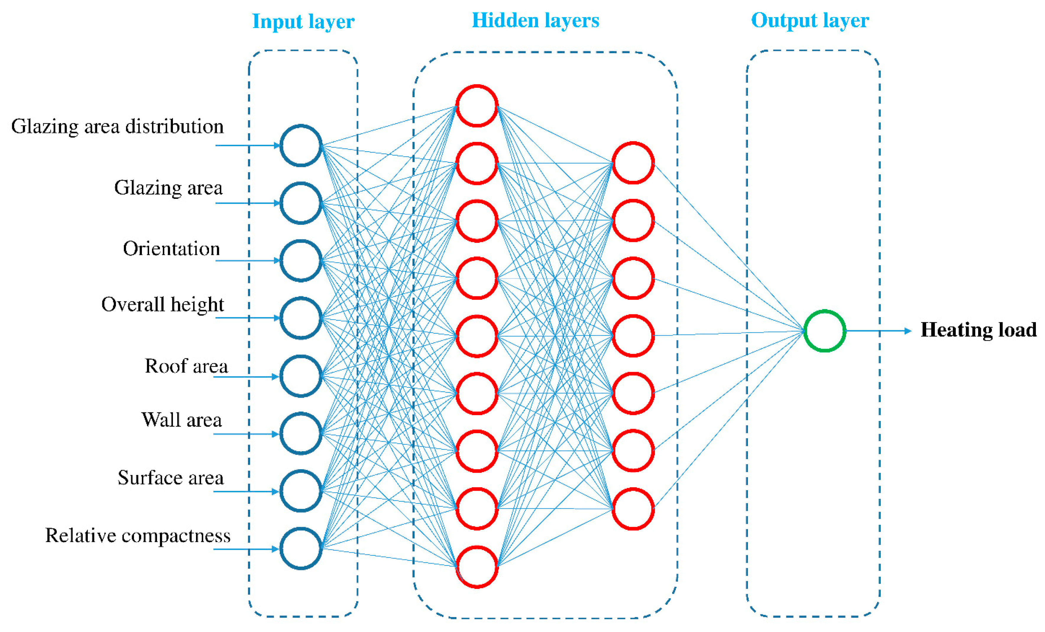
3.5. Artificial Neural Network (ANN)

Based on the human brain operation principle, ANN has been researched and developed as an alternative tool for different social purposes. It is even smarter than the human in some cases, with substantial computing power. In real-life, ANN was studied and applied to solve many problems, such as prediction of self-compacting concrete strength [55], anisotropic masonry failure criterion [56], prediction of the mechanical properties of sandcrete materials [57], blasting issues [58,59,60,61,62,63,64], landslide assessment [65,66,67], to name a few [68,69,70,71,72,73,74,75]. They operate based on data analysis from input neurons, where the input data of the dataset is contained. Here, the information is analyzed and transmitted through hidden layers containing hidden neurons, via the transfer function. In the hidden layers, data is encrypted, analyzed, and calculated through weights. The biases are also estimated to ensure a balanced level of data. Finally, the outcome is computed on the output layer. Figure 5 illustrates the framework of ANN model for predicting the HL of EEB systems in this study based on the eight input variables and one output variable.

4. Evaluation Performance Indices

To evaluate the quality of the PSO-ANN, GA-ANN, ICA-ANN, and ABC-ANN models, R², RMSE, and MAE, were used as the indicators of the model’s performances. They were computed as Equations (4–6):

$$RMSE=\sqrt{\frac{1}{n}{\displaystyle \sum _{i=1}^n(y_i-{\widehat{y}}_i}{)}^2}$$

(4)

$$R^2=1-\frac{{\displaystyle \sum _{i=1}^n{(y_i-{\widehat{y}}_i)}^2}}{{\displaystyle \sum _{i=1}^n{(y_i-\overline{y})}^2}}$$

(5)

$$MAE=\frac{1}{n}{\displaystyle \sum _{i=1}^n\left|y_i-{\widehat{y}}_i\right|}$$

(6)

n stands for the number of instances; $\overline{y}$, $y_i$, and ${\widehat{y}}_i$ are considered as average, calculated, and modeled amounts of the response variable.

5. Prediction of Heating Load (HL) by the Genetic Algorithm-Artificial Neural Network (GA-ANN) Model

Before predicting the HL of EEB systems by the stated models, the dataset was split into two clusters, i.e., training and testing. According to the previous studies, the original dataset should be divided into two parts by randomly according to the 80/20 ratio [76,77]. Thus, for the training process, 80% of the whole dataset (672 experimental datasets) was selected randomly to develop the models. The remaining 20% (165 experimental datasets) was used for the testing process, which is the method for evaluating the quality/performance of the GA-ANN, PSO-ANN, ICA-ANN, and ABC-ANN models.

For the prediction of HL of EEB systems by the GA-ANN model, an initialization ANN model was developed first; then, the GA was used to optimize the developed ANN model, where the weights and biases were optimized. According to Nguyen et al. [68], one or two hidden layers of the ANN model can implement very well all regression problems. Therefore, a “trial and error” (TAE) procedure was conducted with one and two hidden layers of ANN models. To avoid overfitting of the initial ANN model, the min-max scale method was applied with the scale lies in the range of [−1,1]. Ultimately, the ANN model 8-24-18-1 was defined as the best ANN technique for predicting HL of EEB systems in this study. This was the moment for the optimization of the weights and biases of the ANN 8-24-18-1 model by the GA. The number of populations (p), crossover probability (P_c), mutation probability (P_m), and the number variable (n), are the parameters of the GA, that needed to be set up before optimizing herein. In this study, the TAE procedure of p with different values was conducted, i.e., p = 100, 200, 300, 400, 500; P_m was set equal to 0.1; P_c was set equal to 0.9; n = 4. To evaluate the performance of the optimization process, RMSE was used as the fitness function according to Equation (4). The searching operation were performed in 1000 iterations to ensure the optimal searching for the weights and biases of the selected ANN model. The optimal values of weight and bias for the ANN 8-24-18-1 model after optimizing by the GA (i.e., GA-ANN model), were corresponding to the lowest RMSE. The performance of the optimization process by the GA for the ANN 8-24-18-1 model is shown in Figure 6. The final ANN model, after optimized by the GA (i.e., GA-ANN model), is shown in Figure 7.

As stated above, 672 experimental datasets were investigated and analyzed to develop the models. The back-propagation algorithm was applied to training the GA-ANN model. Note that the min-max scale with the range [−1,1] was used for all the models to avoid underfitting/overfitting. The performance of the training process for predicting HL of EEB systems is interpreted in Figure 8. Subsequently, 165 experimental datasets were used to evaluate GA-ANN performance as the new dataset. The results of HL prediction on the new data (i.e., 165 experimental datasets) were estimated by the developed GA-ANN model and are shown in Figure 9.

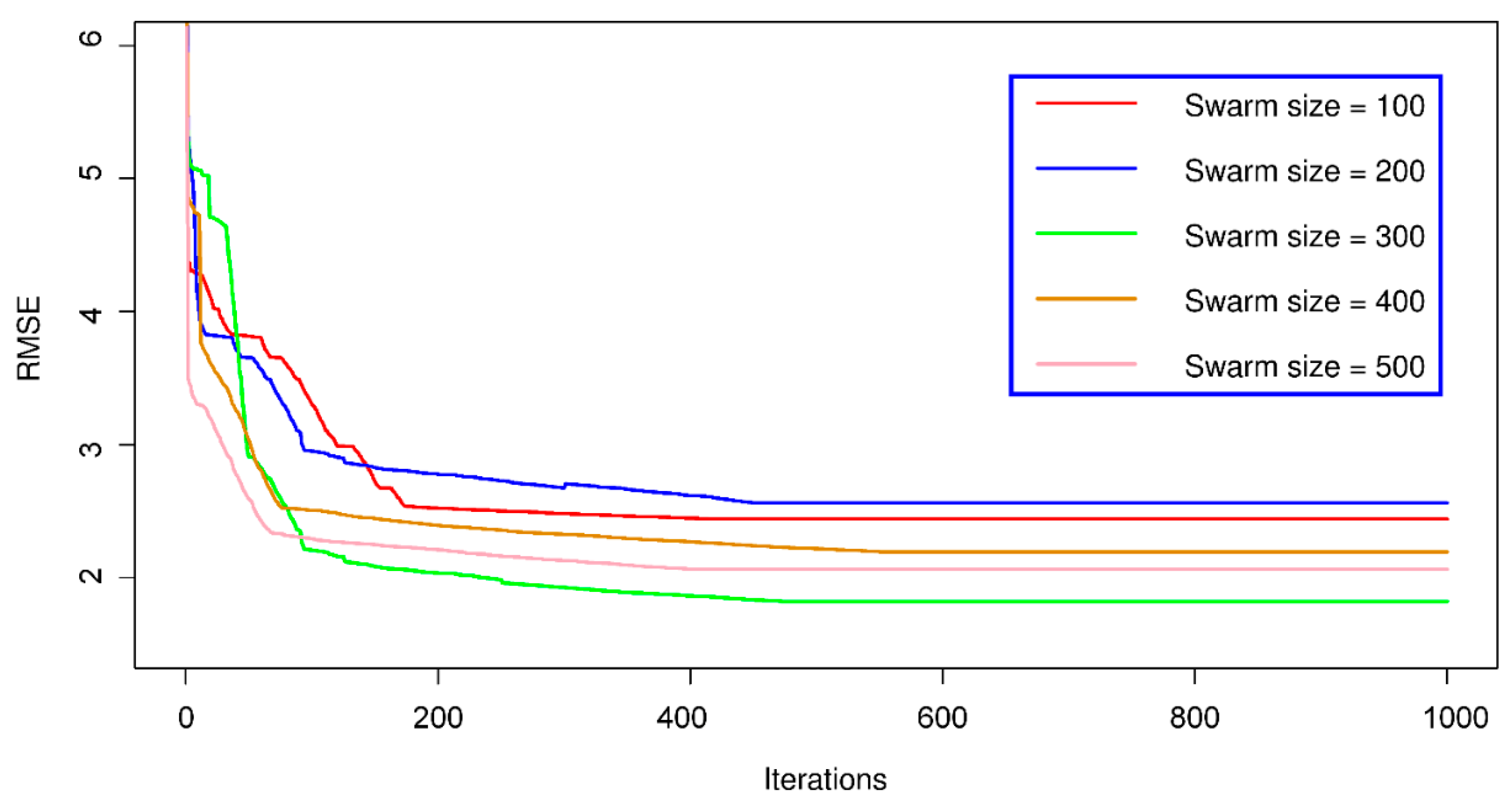
6. Prediction of HL by the Particle Swarm Optimization (PSO)-ANN Model

Like the GA-ANN model, the selected initialization ANN model was optimized by the PSO algorithm for predicting HL of EEB systems, called PSO-ANN model. In this regard, the parameters of the PSO algorithm were set up before optimization of the ANN model (i.e., ANN 8-24-18-1 model), including the number of particle swarms (Sw), maximum particle’s velocity (V_max), individual cognitive (${\varphi }_1$), group cognitive(${\varphi }_2$), inertia weight (w), and maximum number of iteration (m_i). Then, the weights and biases of the initialization ANN model were optimized by the PSO algorithms, as those applied for the GA-ANN model above. Similar to the GA-ANN model, a TAE procedure of Sw was implemented, with Sw of 100, 200, 300, 400, 500, respectively; V_max = 1.8; ${\varphi }_1$ = ${\varphi }_2$= 1.7; w = 1.8, and m_i = 1000. The similar techniques as those used for the GA-ANN model were also applied for the PSO-ANN model in developing the model (i.e., back-propagation algorithm, min-max scale [−1,1]). Finally, the best PSO-ANN model was determined with the lowest RMSE. Figure 10 shows the performance of the PSO-ANN model in the training process. Figure 11 illustrates the structure of the PSO-ANN model. Note that, although the number of input neurons, hidden layers, and neurons, as well as the output layer, is the same as Figure 8; however, the weights and biases of them are different. Eventually, the HL predictions on the training dataset and testing dataset were conducted based on the developed PSO-ANN model, as shown in Figure 12 and Figure 13, respectively.

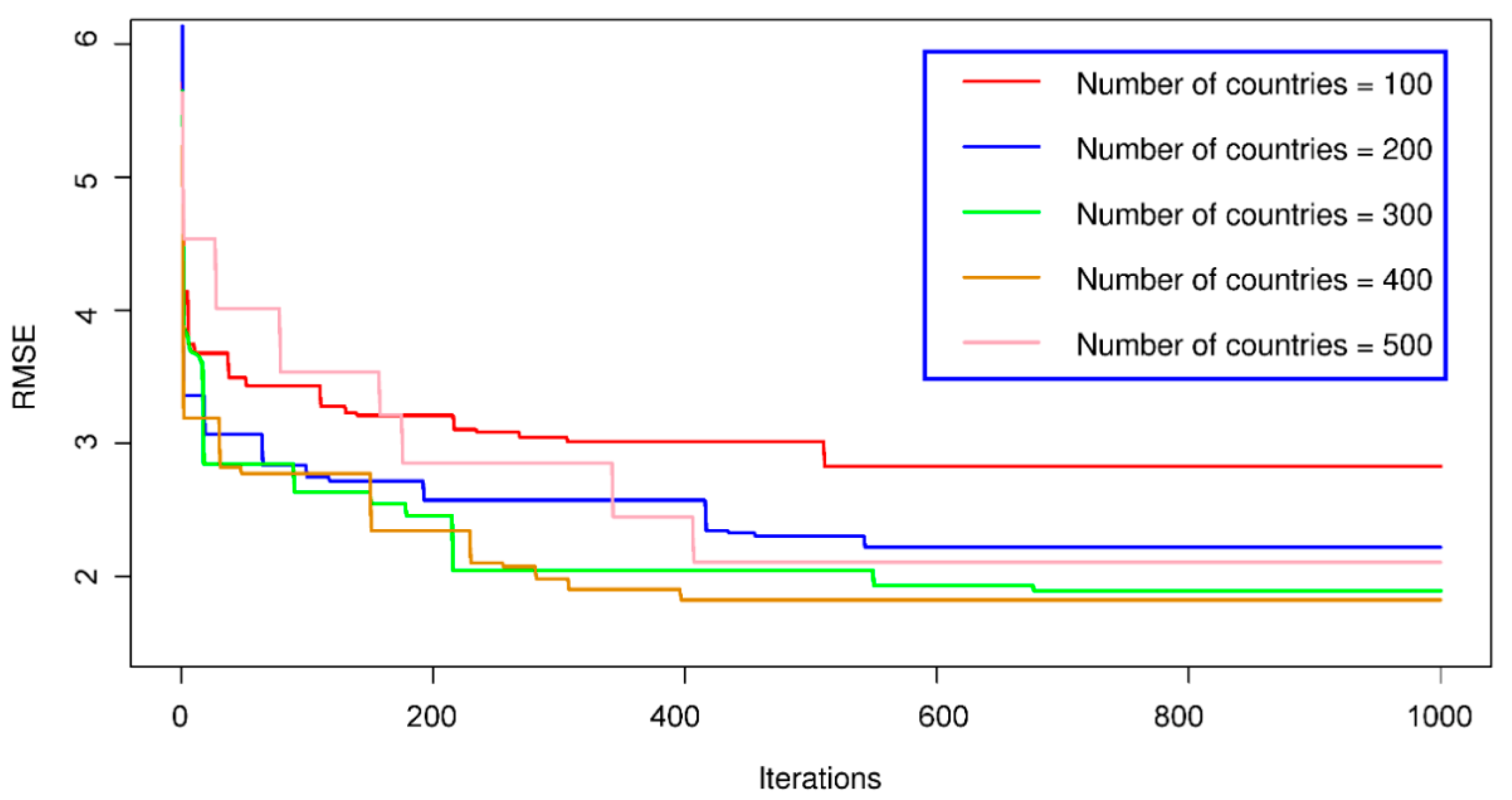
7. Prediction of HL by the Imperialist Competitive Algorithm (ICA)-ANN Model

In this section, the HL of EEB systems was predicted by the ICA-ANN model. As those applied for the GA-ANN and PSO-ANN model, the ICA was used to optimize the weights and biases of the selected initialization ANN model (i.e., ANN 8-24-18-1 model). The parameters of ICA are also needed to be set up before optimization of the ANN model, including the number of initial countries (N_country), initial imperialists (N_imper), maximum number of iterations (N_i), lower-upper limit of the optimization region (L), assimilation coefficient (As), and revolution of each country (r). For implementing this task, a TAE procedure was also applied for N_country, with N_country set equal to 100, 200, 300, 400, 500, respectively; N_imper was set equal to 10, 20, 30, respectively; L was set in the rage of [−10,10]; As equal to 3; r as to 0.5, and N_i was set equal to 1000. Afterward, the emperies perform a global search for the colonies (e.g., weights and biases). The fitness of the emperies was assessed through RMSE. The best ICA-ANN model is associated with the lowest RMSE. Figure 14 shows the performance of the optimization process by the ICA for the ANN model. Ultimately, the final ICA-ANN model was found, as shown in Figure 15. Note that the structure of the developed ICA-ANN model is the same with the GA-ANN and PSO-ANN models; however, the weights and biases (e.g., black and grey lines) of them are different. Additionally, the similar techniques as those used for the GA-ANN and PSO-ANN models were also applied for the ICA-ANN model in developing the model (i.e., back-propagation algorithm, min-max scale [−1,1]).

Based on the ICA-ANN model developed, the outcome of HL predictions was performed. Figure 16 shows the HL predictions of the training dataset when the development of the ICA-ANN model. Applying the ICA-ANN model developed, the new dataset includes 165 experimental datasets on the testing dataset was used to check the quality of the model, like those tested for the GA-ANN and PSO-ANN models. The results of the HL predictions on the new dataset (testing dataset) are shown in Figure 17.

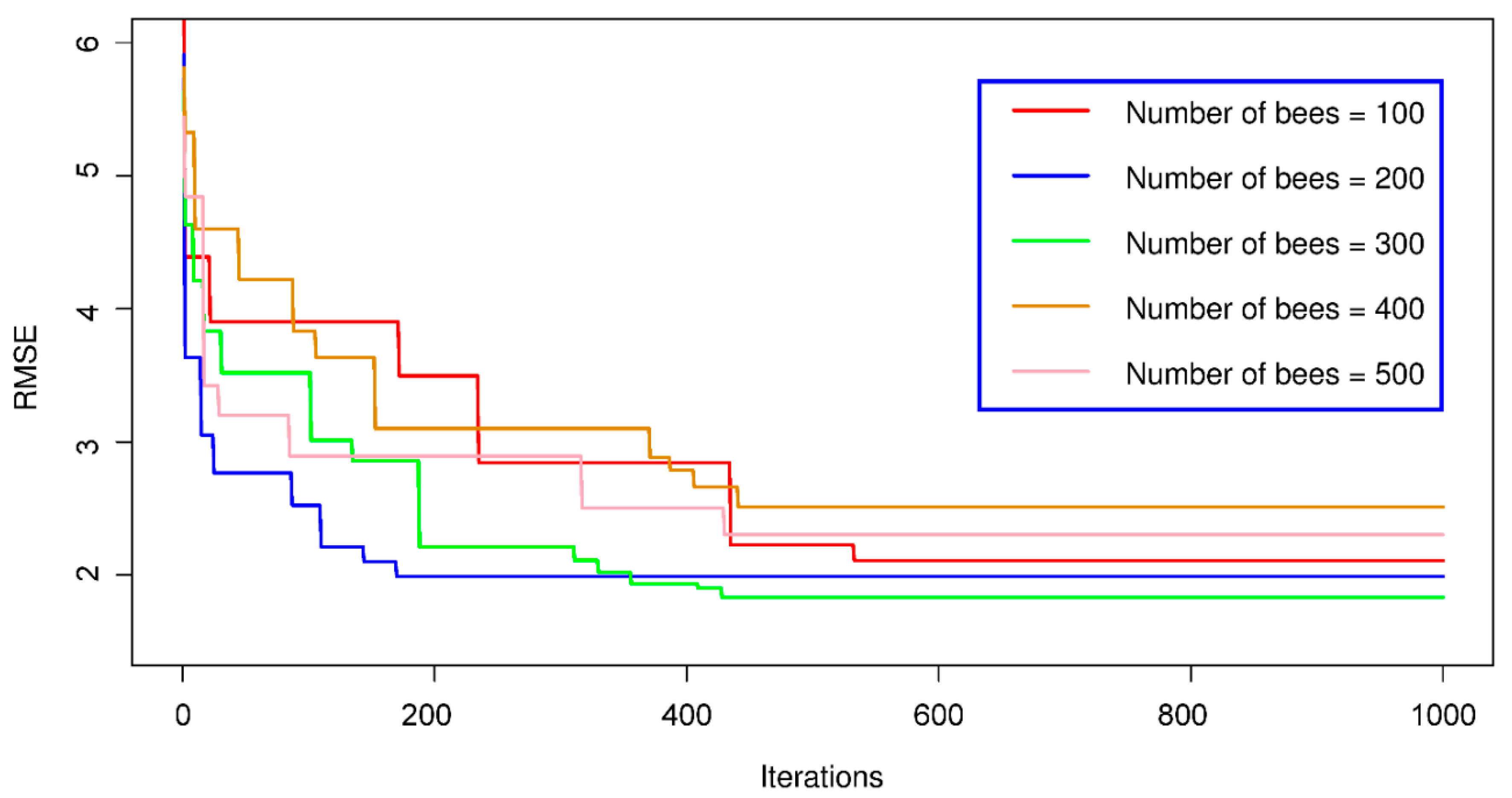
8. Prediction of HL by the Artificial Bee Colony (ABC)-ANN Model

For the HL predictions by the ABC-ANN model, a process of the development of the hybrid model was conducted, similar to those models above (e.g., ICA-ANN, PSO-ANN, GA-ANN). Accordingly, the ABC algorithm was applied to optimize the parameters of the selected ANN model (i.e., ANN 8-24-18-1 model), for predicting HL of EEB systems. The initial setting for the ABC algorithm is necessary, as with those set for the previous models (e.g., ICA-ANN, PSO-ANN, GA-ANN), including the number of bees (N_bees), the number of food sources (N_foodsource), the limit of a food source (M_foodsource), the boundary of the parameters (b), and the maximum number of repetitions for optimization (nround). Similar to the GA, PSO, and ICA, a TAE procedure for in the ABC algorithm was conducted, with N_bees = 100, 200, 300, 400, 500, respectively. The other parameters of the ABC algorithm were set as follow: N_foodsource = 50; M_foodsource =100; b = [−10;10], and nround = 1000. Once the parameters of the ABC algorithms were established, the initialization ANN model 8–24–18–1 model was optimized by the global search of the bee colony. RMSE was also used to evaluate the efficiency of the optimization of the ABC-ANN model, with the optimal ABC-ANN model corresponding to the lowest RMSE. Figure 18 presents the performance of the optimization process of the ABC-ANN model in estimating the HL of EEB systems. Finally, the optimal ABC-ANN model was defined with the optimal weights and biases, as shown in Figure 19.

It should be noted that although Figure 7, Figure 11, Figure 15 and Figure 19 are the same, their structure is different since the weights and biases of the models are different. In addition, similar techniques as those used for the ICA-ANN, PSO-ANN, and GA-ANN models were also applied for the development of the ABC-ANN model (i.e., back-propagation algorithm, min-max scale [−1,1]). Figure 20 shows the HL predictions of the ABC-ANN model on the training dataset. Then, 165 experimental datasets were predicted based on the developed ABC-ANN models, as shown in Figure 21.

9. Comparison and Evaluation of the Developed Models

After the models were developed and HL of EEB systems was predicted, their results were compared and evaluated together through the performance metrics (e.g., RMSE, R², and MAE), and the intensity of color and ranking methods. A comprehensive assessment of the developed models based on both training and the testing dataset was conducted in this section.

Table 2. Prediction results of the hybrid models and their performance (for the training process).

Model	RMSE	R2	MAE	Rank for RMSE	Rank for R2	Rank for MAE	Total Ranking
GA-ANN	1.701	0.972	0.784	4	2	4	10
PSO-ANN	1.822	0.972	0.872	3	2	1	6
ICA-ANN	1.847	0.971	0.860	1	1	2	4
ABC-ANN	1.833	0.972	0.813	2	2	3	7

presents the prediction results of HL by the hybrid intelligent techniques (i.e., GA-ANN, ABC-ANN, PSO-ANN, and ICA-ANN), and their performance in the training process.

From Table 2, the color intensity revealed that the GA-ANN model provided the most dominant performance in the training process. It obtained the lowest error with an RMSE of 1.701, R² of 0.972, and MAE of 0.784, and the total ranking of 10, on the training dataset. The ABC and PSO meta-heuristics algorithms yielded lower performance in the optimization of the ANN model in the training process, with RMSE of 1.833, 1.822; R² of 0.927, 0.972; MAE of 0.813, 0.872, and the total ranking of 7, and 6, respectively. The weakest model in this optimization process is the ICA-ANN model with an RMSE of 1.847, R² of 0.971, MAE of 0.860, and the total ranking of 4. To have a complete conclusion, the models’ performances were assessed on the testing dataset, where the dataset was considered as the new data and ever not used in the training process.

Table 3. Prediction results of the hybrid models and their performance (for the testing process).

Model	RMSE	R2	MAE	Rank for RMSE	Rank for R2	Rank for MAE	Total Ranking
GA-ANN	1.625	0.980	0.798	4	4	4	12
PSO-ANN	1.932	0.972	1.027	2	2	1	5
ICA-ANN	1.982	0.970	0.980	1	1	2	4
ABC-ANN	1.878	0.973	0.957	3	3	3	9

shows the results and the performance of the models in the testing process.

Based on the reports of Table 3, similar results to the training process were reflected. The color intensity of the red color indicated that the GA-ANN model was the best model in a comparison of the other models. The corresponding performance values of the GA-ANN model also found with an RMSE of 1.625, R² of 0.980, MAE of 0.798, and the total ranking of 12. Whereas, the ABC-ANN, PSO-ANN, and ICA-ANN model proved lower performances, as like the training process, with RMSE of 1.878, 1.932, 1.982; R² of 0.973, 0.972, 0.970; MAE of 0.957, 1.027, 0.980; and the total ranking of 9, 5, 4, respectively.

10. Sensitivity Analysis

To get an overall conclusion and optimization solutions in building design aim to use energy-efficiency, the importance level of the input variables for predicting HL in the present work was conducted. The initial ANN model (i.e., ANN 8-24-18-1) was investigated using the Olden method [78] to analyze the importance of the input variables. This method enables the analysis of the importance of input variables for hidden multiple-layer ANN models [79]. Ultimately, the importance level of the input variables for predicting HL of EEB systems was determined, as shown in Figure 22. Based on the sensitivity analysis results of this study, it can be seen that GAD, SA, GA, RA, OH, and WA, were the most important variables in predicting the HL of EEB systems, especially SA and GA.

11. Conclusions

Energy efficiency is one of the essential requirements for smart cities. Artificial intelligence has also been considered as powerful support tools for these objectives in smart cities. This study developed and proposed four new hybrid models based on AI techniques for estimating the HL of EEB systems with high reliability, i.e., GA-ANN, PSO-ANN, ICA-ANN, and ABC-ANN models. A comprehensive comparison and assessment of the developed models were performed in this work. As a conclusion, the meta-heuristics algorithms performed very well in the optimization of the ANN model. Of the meta-heuristics algorithms used in this study, the GA provided the highest performance in optimizing the ANN model, to predict the HL of EEB systems, i.e., GA-ANN model. The remaining meta-heuristics algorithms (i.e., PSO, ICA, ABC) provided more unsatisfactory performance, corresponding to the performance of the PSO-ANN, ICA-ANN, and ABC-ANN models.

Based on the results of this study, the HL of EEB can be accurately predicted and controlled to ensure the energy efficiency of buildings in smart cities. Software or applications on computers and smartphones can be developed in the future based on the results of this study for the use of energy saving and efficiency of buildings in smart cities. Besides, it can also be integrated into smart houses to adjust and control the HL of the houses automatically. Furthermore, optimization techniques of building design, as well as smart city planning, can also be conducted based on the models developed in this study. Notably, the GAD, SA, GA, RA, OH, and WA are the main parameters which should be carefully concerned and calculated in designing buildings and smart cities. Based on the results of this study as well as software or applications on smartphones and computers, engineers can optimize the building parameters to use HL in smart cities effectively.

References

1. Cocchia, A. Smart and digital city: A systematic literature review. In Smart City: How to Create Public and Economic Value with High Technology in Urban Space; Dameri, R.P., Rosenthal-Sabroux, C., Eds.; Springer International Publishing: Cham, Switzerland; pp. 13–43. [CrossRef]
2. Anthopoulos, L.G. Understanding the smart city domain: A literature review. In Transforming City Governments for Successful Smart Cities; Rodríguez-Bolívar, M.P., Ed.; Springer International Publishing: Cham, Switzerland; pp. 9–21. [CrossRef]
3. Caragliu, A.; Del Bo, C.; Nijkamp, P. Smart cities in Europe. J. Urban Technol. 2011, 18, 65–82. [Google Scholar] [CrossRef]
4. Bibri, S.E.; Krogstie, J. Smart sustainable cities of the future: An extensive interdisciplinary literature review. Sustain. Cities Soc. 2017, 31, 183–212. [Google Scholar] [CrossRef]
5. Talari, S.; Shafie-Khah, M.; Siano, P.; Loia, V.; Tommasetti, A.; Catalão, J. A review of smart cities based on the internet of things concept. Energies 2017, 10, 421. [Google Scholar] [CrossRef]
6. Silva, B.N.; Khan, M.; Han, K. Towards sustainable smart cities: A review of trends, architectures, components, and open challenges in smart cities. Sustain. Cities Soc. 2018, 38, 697–713. [Google Scholar] [CrossRef]
7. Esmaeilian, B.; Wang, B.; Lewis, K.; Duarte, F.; Ratti, C.; Behdad, S. The future of waste management in smart and sustainable cities: A review and concept paper. Waste Manag. 2018, 81, 177–195. [Google Scholar] [CrossRef] [PubMed]
8. Martin, C.J.; Evans, J.; Karvonen, A. Smart and sustainable? Five tensions in the visions and practices of the smart-sustainable city in Europe and North America. Technol. Forecast. Soc. Chang. 2018, 133, 269–278. [Google Scholar] [CrossRef]
9. Zhao, H.-X.; Magoulès, F. A review on the prediction of building energy consumption. Renew. Sustain. Energy Rev. 2012, 16, 3586–3592. [Google Scholar] [CrossRef]
10. Catalina, T.; Iordache, V.; Caracaleanu, B. Multiple regression model for fast prediction of the heating energy demand. Energy Build. 2013, 57, 302–312. [Google Scholar] [CrossRef]
11. Chou, J.-S.; Bui, D.-K. Modeling heating and cooling loads by artificial intelligence for energy-efficient building design. Energy Build. 2014, 82, 437–446. [Google Scholar] [CrossRef]
12. Rubin, D.B. Iteratively Reweighted Least Squares; Encyclopedia of Statistical Sciences, © John Wiley & Sons, Inc. and republished in Wiley StatsRef: Statistics Reference Online, 2014. [Google Scholar] [CrossRef]
13. Tsanas, A.; Xifara, A. Accurate quantitative estimation of energy performance of residential buildings using statistical machine learning tools. Energy Build. 2012, 49, 560–567. [Google Scholar] [CrossRef]
14. Castelli, M.; Trujillo, L.; Vanneschi, L.; Popovič, A. Prediction of energy performance of residential buildings: A genetic programming approach. Energy Build. 2015, 102, 67–74. [Google Scholar] [CrossRef]
15. Fan, C.; Xiao, F.; Zhao, Y. A short-term building cooling load prediction method using deep learning algorithms. Appl. Energy 2017, 195, 222–233. [Google Scholar] [CrossRef]
16. Ascione, F.; Bianco, N.; De Stasio, C.; Mauro, G.M.; Vanoli, G.P. Artificial neural networks to predict energy performance and retrofit scenarios for any member of a building category: A novel approach. Energy 2017, 118, 999–1017. [Google Scholar] [CrossRef]
17. Ngo, N.-T. Early predicting cooling loads for energy-efficient design in office buildings by machine learning. Energy Build. 2019, 182, 264–273. [Google Scholar] [CrossRef]
18. Nguyen, H.; Moayedi, H.; Jusoh, W.A.W.; Sharifi, A. Proposing a novel predictive technique using M5Rules-PSO model estimating cooling load in energy-efficient building system. Eng. Comput. 2019, 1–10. [Google Scholar] [CrossRef]
19. Bui, X.-N.; Moayedi, H.; Rashid, A.S.A. Developing a predictive method based on optimized M5Rules–GA predicting heating load of an energy-efficient building system. Eng. Comput. 2019, 1–10. [Google Scholar] [CrossRef]
20. Pino-Mejías, R.; Pérez-Fargallo, A.; Rubio-Bellido, C.; Pulido-Arcas, J.A. Comparison of linear regression and artificial neural networks models to predict heating and cooling energy demand, energy consumption and CO2 emissions. Energy 2017, 118, 24–36. [Google Scholar] [CrossRef]
21. Idowu, S.; Saguna, S.; Åhlund, C.; Schelén, O. Applied machine learning: Forecasting heat load in district heating system. Energy Build. 2016, 133, 478–488. [Google Scholar] [CrossRef]
22. Roy, S.S.; Roy, R.; Balas, V.E. Estimating heating load in buildings using multivariate adaptive regression splines, extreme learning machine, a hybrid model of MARS and ELM. Renew. Sustain. Energy Rev. 2018, 82, 4256–4268. [Google Scholar]
23. Wang, L.; Kubichek, R.; Zhou, X. Adaptive learning based data-driven models for predicting hourly building energy use. Energy Build. 2018, 159, 454–461. [Google Scholar] [CrossRef]
24. Niemierko, R.; Töppel, J.; Tränkler, T. A D-vine copula quantile regression approach for the prediction of residential heating energy consumption based on historical data. Appl. Energy 2019, 233, 691–708. [Google Scholar] [CrossRef]
25. Bui, X.-N.; Muazu, M.A.; Nguyen, H. Optimizing Levenberg–Marquardt backpropagation technique in predicting factor of safety of slopes after two-dimensional OptumG2 analysis. Eng. Comput. 2019, 35, 813–832. [Google Scholar] [CrossRef]
26. Moayed, H.; Rashid, A.S.A.; Muazu, M.A.; Nguyen, H.; Bui, X.-N.; Bui, D.T. Prediction of ultimate bearing capacity through various novel evolutionary and neural network models. Eng. Comput. 2019, 1–17. [Google Scholar] [CrossRef]
27. Zhang, X.; Nguyen, H.; Bui, X.-N.; Tran, Q.-H.; Nguyen, D.-A.; Bui, D.T.; Moayedi, H. Novel Soft Computing Model for Predicting Blast-Induced Ground Vibration in Open-Pit Mines Based on Particle Swarm Optimization and XGBoost. Nat. Resour. Res. 2019, 1–11. [Google Scholar] [CrossRef]
28. Moayedi, H.; Raftari, M.; Sharifi, A.; Jusoh, W.A.W.; Rashid, A.S.A. Optimization of ANFIS with GA and PSO estimating α ratio in driven piles. Eng. Comput. 2019. [Google Scholar] [CrossRef]
29. Nguyen, H.; Moayedi, H.; Foong, L.K.; Al Najjar, H.A.H.; Jusoh, W.A.W.; Rashid, A.S.A.; Jamali, J. Optimizing ANN models with PSO for predicting short building seismic response. Eng. Comput. 2019, 1–15. [Google Scholar] [CrossRef]
30. Armaghani, D.J.; Hajihassani, M.; Marto, A.; Faradonbeh, R.S.; Mohamad, E.T. Prediction of blast-induced air overpressure: A hybrid AI-based predictive model. Environ. Monit. Assess. 2015, 187, 666. [Google Scholar] [CrossRef]
31. Armaghani, D.J.; Hasanipanah, M.; Mahdiyar, A.; Majid, M.Z.A.; Amnieh, H.B.; Tahir, M.M. Airblast prediction through a hybrid genetic algorithm-ANN model. Neural Comput. Appl. 2016, 29, 619–629. [Google Scholar] [CrossRef]
32. Armaghani, D.J.; Mohamad, E.T.; Narayanasamy, M.S.; Narita, N.; Yagiz, S. Development of hybrid intelligent models for predicting TBM penetration rate in hard rock condition. Tunn. Undergr. Space Technol. 2017, 63, 29–43. [Google Scholar] [CrossRef]
33. Zhou, J.; Nekouie, A.; Arslan, C.A.; Pham, B.T.; Hasanipanah, M. Novel approach for forecasting the blast-induced AOp using a hybrid fuzzy system and firefly algorithm. Eng. Comput. 2019, 1–10. [Google Scholar] [CrossRef]
34. Asteris, P.G.; Nozhati, S.; Nikoo, M.; Cavaleri, L.; Nikoo, M. Krill herd algorithm-based neural network in structural seismic reliability evaluation. Mech. Adv. Mater. Struct. 2018, 1–8. [Google Scholar] [CrossRef]
35. Asteris, P.G.; Nikoo, M. Artificial bee colony-based neural network for the prediction of the fundamental period of infilled frame structures. Neural Comput. Appl. 2019, 1–11. [Google Scholar] [CrossRef]
36. Eberhart Kennedy, J. A new optimizer using particle swarm theory. In Proceedings of the Sixth International Symposium on Micro Machine and Human Science (MHS’95), Nagoya, Japan, 4–6 October 1995; pp. 39–43. [Google Scholar]
37. Armaghani, D.J.; Hajihassani, M.; Mohamad, E.T.; Marto, A.; Noorani, S.A. Blasting-induced flyrock and ground vibration prediction through an expert artificial neural network based on particle swarm optimization. Arab. J. Geosci. 2014, 7, 5383–5396. [Google Scholar] [CrossRef]
38. Gordan, B.; Armaghani, D.J.; Hajihassani, M.; Monjezi, M. Prediction of seismic slope stability through combination of particle swarm optimization and neural network. Eng. Comput. 2016, 32, 85–97. [Google Scholar] [CrossRef]
39. Yang, X.; Zhang, Y.; Yang, Y.; Lv, W. Deterministic and Probabilistic Wind Power Forecasting Based on Bi-Level Convolutional Neural Network and Particle Swarm Optimization. Appl. Sci. 2019, 9, 1794. [Google Scholar] [CrossRef]
40. Kulkarni, R.V.; Venayagamoorthy, G.K. An estimation of distribution improved particle swarm optimization algorithm. In Proceedings of the 2007 3rd International Conference on Intelligent Sensors, Sensor Networks and Information, Melbourne, QLD, Australia, 3–6 December 2007; pp. 539–544. [Google Scholar]
41. Mitchell, M. An Introduction to Genetic Algorithms; MIT Press: Cambridge, MA, USA; London, England, 1998. [Google Scholar]
42. Carr, J. An introduction to genetic algorithms. Sr. Proj. 2014, 1, 40. [Google Scholar]
43. Kinnear, K.E., Jr. A perspective on the work in this book. In Advances in Genetic Programming; MIT Press: Cambridge, MA, USA; London, England, 1994; pp. 3–19. [Google Scholar]
44. Raeisi-Vanani, H.; Shayannejad, M.; Soltani-Toudeshki, A.-R.; Arab, M.-A.; Eslamian, S.; Amoushahi-Khouzani, M.; Marani-Barzani, M.; Ostad-Ali-Askari, K. A Simple Method for Land Grading Computations and its Comparison with Genetic Algorithm (GA) Method. Int. J. Res. Stud. Agric. Sci. 2017, 3, 26–38. [Google Scholar]
45. Goldberg, D. Genetic Algorithms in Search, Optimization, and Machine Language; Addison-Wesley: Reading, UK, 1989. [Google Scholar]
46. Zheng, Y.; Huang, M.; Lu, Y.; Li, W. Fractional stochastic resonance multi-parameter adaptive optimization algorithm based on genetic algorithm. Neural Comput. Appl. 2018, 1–12. [Google Scholar] [CrossRef]
47. Atashpaz-Gargari, E.; Lucas, C. Imperialist competitive algorithm: An algorithm for optimization inspired by imperialistic competition. In Proceedings of the 2007 IEEE Congress on Evolutionary computation, Singapore, 25–28 September 2007; pp. 4661–4667. [Google Scholar]
48. Hosseini, S.; Al Khaled, A. A survey on the imperialist competitive algorithm metaheuristic: Implementation in engineering domain and directions for future research. Appl. Soft Comput. 2014, 24, 1078–1094. [Google Scholar] [CrossRef]
49. Elsisi, M. Design of neural network predictive controller based on imperialist competitive algorithm for automatic voltage regulator. Neural Comput. Appl. 2019, 1–11. [Google Scholar] [CrossRef]
50. Zadeh Shirazi, A.; Mohammadi, Z. A hybrid intelligent model combining ANN and imperialist competitive algorithm for prediction of corrosion rate in 3C steel under seawater environment. Neural Comput. Appl. 2017, 28, 3455–3464. [Google Scholar] [CrossRef]
51. Karaboga, D. An Idea Based on Honey Bee Swarm for Numerical Optimization; Technical Report-tr06; Erciyes University, Engineering Faculty, Computer Engineering Department: Melikgazi/Kayseri, Turkey, 2005. [Google Scholar]
52. Zhong, F.; Li, H.; Zhong, S. An improved artificial bee colony algorithm with modified-neighborhood-based update operator and independent-inheriting-search strategy for global optimization. Eng. Appl. Artif. Intell. 2017, 58, 134–156. [Google Scholar] [CrossRef]
53. Jadon, S.S.; Bansal, J.C.; Tiwari, R.; Sharma, H. Artificial bee colony algorithm with global and local neighborhoods. Int. J. Syst. Assur. Eng. Manag. 2018, 9, 589–601. [Google Scholar] [CrossRef]
54. Ning, J.; Zhang, B.; Liu, T.; Zhang, C. An archive-based artificial bee colony optimization algorithm for multi-objective continuous optimization problem. Neural Comput. Appl. 2018, 30, 2661–2671. [Google Scholar] [CrossRef]
55. Asteris, P.; Kolovos, K.; Douvika, M.; Roinos, K. Prediction of self-compacting concrete strength using artificial neural networks. Eur. J. Environ. Civ. Eng. 2016, 20 (Suppl. 1), s102–s122. [Google Scholar] [CrossRef]
56. Asteris, P.G.; Plevris, V. Anisotropic masonry failure criterion using artificial neural networks. Neural Comput. Appl. 2017, 28, 2207–2229. [Google Scholar] [CrossRef]
57. Asteris, P.; Roussis, P.; Douvika, M. Feed-forward neural network prediction of the mechanical properties of sandcrete materials. Sensors 2017, 17, 1344. [Google Scholar] [CrossRef] [PubMed]
58. Dimitraki, L.; Christaras, B.; Marinos, V.; Vlahavas, I.; Arampelos, N. Predicting the average size of blasted rocks in aggregate quarries using artificial neural networks. Bull. Eng. Geol. Environ. 2019, 78, 2717–2729. [Google Scholar] [CrossRef]
59. Armaghani, D.J.; Hasanipanah, M.; Mohamad, E.T. A combination of the ICA-ANN model to predict air-overpressure resulting from blasting. Eng. Comput. 2016, 32, 155–171. [Google Scholar] [CrossRef]
60. Armaghani, D.J.; Momeni, E.; Abad, S.V.A.N.K.; Khandelwal, M. Feasibility of ANFIS model for prediction of ground vibrations resulting from quarry blasting. Environ. Earth Sci. 2015, 74, 2845–2860. [Google Scholar] [CrossRef] [Green Version]
61. Nguyen, H.; Bui, X.-N. Predicting Blast-Induced Air Overpressure: A Robust Artificial Intelligence System Based on Artificial Neural Networks and Random Forest. Nat. Resour. Res. 2018, 28, 893–907. [Google Scholar] [CrossRef]
62. Nguyen, H.; Bui, X.-N.; Bui, H.-B.; Mai, N.-L. A comparative study of artificial neural networks in predicting blast-induced air-blast overpressure at Deo Nai open-pit coal mine, Vietnam. Neural Comput. Appl. 2018, 1–17. [Google Scholar] [CrossRef]
63. Nguyen, H.; Bui, X.-N.; Tran, Q.-H.; Le, T.-Q.; Do, N.-H.; Hoa, L.T.T. Evaluating and predicting blast-induced ground vibration in open-cast mine using ANN: A case study in Vietnam. SN Appl. Sci. 2018, 1, 125. [Google Scholar] [CrossRef]
64. Nguyen, H.; Drebenstedt, C.; Bui, X.-N.; Bui, D.T. Prediction of Blast-Induced Ground Vibration in an Open-Pit Mine by a Novel Hybrid Model Based on Clustering and Artificial Neural Network. Nat. Resour. Res. 2019, 1–19. [Google Scholar] [CrossRef]
65. Dou, J.; Yamagishi, H.; Pourghasemi, H.R.; Yunus, A.P.; Song, X.; Xu, Y.; Zhu, Z. An integrated artificial neural network model for the landslide susceptibility assessment of Osado Island, Japan. Nat. Hazards 2015, 78, 1749–1776. [Google Scholar] [CrossRef]
66. Dou, J.; Paudel, U.; Oguchi, T.; Uchiyama, S.; Hayakavva, Y.S. Shallow and Deep-Seated Landslide Differentiation Using Support Vector Machines: A Case Study of the Chuetsu Area, Japan. Terr. Atmos. Ocean. Sci. 2015, 26, 227–239. [Google Scholar] [CrossRef]
67. Oh, H.-J.; Lee, S. Shallow landslide susceptibility modeling using the data mining models artificial neural network and boosted tree. Appl. Sci. 2017, 7, 1000. [Google Scholar] [CrossRef]
68. Nguyen, H.; Bui, X.-N.; Moayedi, H. A comparison of advanced computational models and experimental techniques in predicting blast-induced ground vibration in open-pit coal mine. Acta Geophys. 2019. [Google Scholar] [CrossRef]
69. Asteris, P.G.; Tsaris, A.K.; Cavaleri, L.; Repapis, C.C.; Papalou, A.; Di Trapani, F.; Karypidis, D.F. Prediction of the fundamental period of infilled RC frame structures using artificial neural networks. Comput. Intell. Neurosci. 2016, 2016, 20. [Google Scholar] [CrossRef] [PubMed]
70. Plevris, V.; Asteris, P.G. Modeling of masonry failure surface under biaxial compressive stress using Neural Networks. Constr. Build. Mater. 2014, 55, 447–461. [Google Scholar] [CrossRef]
71. Cavaleri, L.; Chatzarakis, G.E.; Trapani, F.D.; Douvika, M.G.; Roinos, K.; Vaxevanidis, N.M.; Asteris, P.G. Modeling of surface roughness in electro-discharge machining using artificial neural networks. Adv. Mater. Res. 2017, 6, 169–184. [Google Scholar]
72. Ferrero Bermejo, J.; Gómez Fernández, J.F.; Olivencia Polo, F.; Crespo Márquez, A. A Review of the Use of Artificial Neural Network Models for Energy and Reliability Prediction. A Study of the Solar PV, Hydraulic and Wind Energy Sources. Appl. Sci. 2019, 9, 1844. [Google Scholar] [CrossRef]
73. Kim, C.; Lee, J.-Y.; Kim, M. Prediction of the Dynamic Stiffness of Resilient Materials using Artificial Neural Network (ANN) Technique. Appl. Sci. 2019, 9, 1088. [Google Scholar] [CrossRef]
74. Wang, D.-L.; Sun, Q.-Y.; Li, Y.-Y.; Liu, X.-R. Optimal Energy Routing Design in Energy Internet with Multiple Energy Routing Centers Using Artificial Neural Network-Based Reinforcement Learning Method. Appl. Sci. 2019, 9, 520. [Google Scholar] [CrossRef]
75. Azeez, O.S.; Pradhan, B.; Shafri, H.Z.; Shukla, N.; Lee, C.-W.; Rizeei, H.M. Modeling of CO emissions from traffic vehicles using artificial neural networks. Appl. Sci. 2019, 9, 313. [Google Scholar] [CrossRef]
76. Shang, Y.; Nguyen, H.; Bui, X.-N.; Tran, Q.-H.; Moayedi, H. A Novel Artificial Intelligence Approach to Predict Blast-Induced Ground Vibration in Open-Pit Mines Based on the Firefly Algorithm and Artificial Neural Network. Nat. Resour. Res. 2019, 1–15. [Google Scholar] [CrossRef]
77. Nguyen, H. Support vector regression approach with different kernel functions for predicting blast-induced ground vibration: A case study in an open-pit coal mine of Vietnam. SN Appl. Sci. 2019, 1, 283. [Google Scholar] [CrossRef]
78. Olden, J.D.; Joy, M.K.; Death, R.G. An accurate comparison of methods for quantifying variable importance in artificial neural networks using simulated data. Ecol. Model. 2004, 178, 389–397. [Google Scholar] [CrossRef]
79. Olden, J.D.; Jackson, D.A. Illuminating the “black box”: A randomization approach for understanding variable contributions in artificial neural networks. Ecol. Model. 2002, 154, 135–150. [Google Scholar] [CrossRef]
Figure 1. Illustrating the components of building [11].
Applsci 09 02630 g001
Figure 2. Properties of the dataset used for estimating heating load (HL) of buildings’ energy efficiency (EEB) systems.
Applsci 09 02630 g002
Figure 3. Flow chart of a genetic algorithm (GA).
Applsci 09 02630 g003
Figure 4. The framework of the artificial bee colony (ABC) optimization.
Applsci 09 02630 g004
Figure 5. Framework of artificial neural network (ANN) model for estimating heating load (HL) of buildings’ energy efficiency (EEB) systems.
Applsci 09 02630 g005
Figure 6. Genetic algorithm-artificial neural network (GA-ANN) performance for estimating HL of EEB systems.
Applsci 09 02630 g006
Figure 7. Structure of the GA-ANN model for determining HL of EEB systems.
Applsci 09 02630 g007
Figure 8. HL predictions on the training dataset of the GA-ANN model.
Applsci 09 02630 g008
Figure 9. HL predictions on the testing dataset of the GA-ANN model.
Applsci 09 02630 g009
Figure 10. Particle swarm optimization (PSO-ANN) performance for estimating HL of EEB systems in the training process.
Applsci 09 02630 g010
Figure 11. Structure of the PSO-ANN model for estimating HL of EEB systems.
Applsci 09 02630 g011
Figure 12. HL predictions on the training dataset of the PSO-ANN model.
Applsci 09 02630 g012
Figure 13. HL predictions on the testing dataset of the PSO-ANN model.
Applsci 09 02630 g013
Figure 14. Imperialist competitive algorithm (ICA)-ANN performance for estimating HL of EEB systems in the training process.
Applsci 09 02630 g014
Figure 15. Structure of the ICA-ANN model for estimating HL of EEB systems.
Applsci 09 02630 g015
Figure 16. HL predictions on the training dataset of the ICA-ANN model.
Applsci 09 02630 g016
Figure 17. HL predictions on the testing dataset of the ICA-ANN model.
Applsci 09 02630 g017
Figure 18. Artificial bee colony (ABC)-ANN performance for estimating HL of EEB systems in the training process.
Applsci 09 02630 g018
Figure 19. Structure of the ABC-ANN model for estimating HL of EEB systems.
Applsci 09 02630 g019
Figure 20. HL predictions on the training dataset of the ABC-ANN model.
Applsci 09 02630 g020
Figure 21. HL predictions on the testing dataset of the ABC-ANN model.
Applsci 09 02630 g021
Figure 22. Importance level of the input variables for predicting the HL of EEB systems.
Applsci 09 02630 g022