Besinc Pseudo-Schell Model Sources with Circular Coherence

Featured Application

optical trapping, tight focusing, microscopy.

Abstract

Partially coherent sources with non-conventional coherence properties present unusual behaviors during propagation, which have potential application in fields like optical trapping and microscopy. Recently, partially coherent sources exhibiting circular coherence have been introduced and experimentally realized. Among them, the so-called pseudo Schell-model sources present coherence properties that depend only on the difference between the radial coordinates of two points. Here, the intensity and coherence properties of the fields radiated from pseudo Schell-model sources with a degree of coherence of the besinc type are analyzed in detail. A sharpening of the intensity profile is found for the propagated beam by appropriately selecting the coherence parameters. As a possible application, the trapping of different types of dielectric nanoparticles with this kind of beam is described.

1. Introduction

The research for physically realizable partially coherent sources keeps on attracting a considerable interest, due to the advantages that partially coherent beams present over their coherent counterparts in some applications, such as, for instance, free space optical communications [1,2,3], imaging [4], and optical trapping [5,6] (see also [7,8] and references therein).

In the coherence theory the Schell model [9,10], describing sources with shift-invariant coherence properties, has played a crucial role. Schell-model sources can be also produced in a very simple way starting from spatially incoherent sources. Nonetheless, recent advances in different fields require new source models with specific properties to be provided. In this sense, the control of the coherence properties of the source allows to obtain beams with peculiar behaviour of their intensity in propagation [8,11,12,13,14,15,16,17,18,19,20,21,22,23].

In analogy to the Schell model, scalar sources that present shift-invariance only along either the radial or azimuthal coordinate have been recently proposed [18,20,24,25]. Since their coherence properties are shift-invariant only along a polar coordinate, they have been named pseudo-Schell model sources [20,24]. Their cross-spectral density (CSD) can fulfill the non-negativeness condition [10,26], in which case they represent physically realizable sources.

The aim of this work is to analyze the behavior of a type of pseudo-Schell model sources whose coherence properties depend only on the difference of the radial coordinates of two points, so that they show circular coherence properties [15,16]. The degree of coherence has been chosen as a besinc function while a Laguerre-Gaussian profile has been selected for the intensity at the source plane. In this case, a pseudo-modal expansion of these sources has been derived. The intensity and coherence properties of the fields radiated from such sources has been described. For appropriate coherence parameters, a sharpening of the intensity profile occurs within a certain range of propagation distances. It has been shown that this sharpening effect could be exploited for simultaneous trapping of dielectric nanoparticles with either higher or lower refractive index than that of the surrounding medium.

The paper is organized as follows: after this Introduction, in Section 2, a family of pseudo-Schell model sources is presented, its coherence properties are described and a pseudo-modal expansion is obtained; the paraxial propagation of the beams generated from such sources are studied in Section 3, while their trapping capabilities are analyzed in Section 4. The main results of this work are discussed in Section 5. Concluding remarks are summarized in Section 6.

2. Source Model

The CSD function $W\left({\mathbf{r}}_1,{\mathbf{r}}_2,0\right)$, defined as the field correlation at two points ${\mathbf{r}}_j=\left(r_j,{\theta }_j\right)$ with $j=1,2$ across the source plane, can be used to properly describe the spatial coherence properties of a light source [10]. Some years ago, a superposition rule was presented [26,27] to establish a sufficient and necessary condition that any function must fulfill to represent a physically realizable CSD. According to it, $W\left({\mathbf{r}}_1,{\mathbf{r}}_2,0\right)$ is a bona fide CSD provided that it can be written as

$$W\left({\mathbf{r}}_1,{\mathbf{r}}_2,0\right)=\int H^{*}\left({\mathbf{r}}_1,\upsilon \right)H\left({\mathbf{r}}_2,\upsilon \right)\mathrm{d}\upsilon ,$$

(1)

where $H\left({\mathbf{r}}_2,\upsilon \right)$ is a kernel that, in this work, has been chosen as

$$H\left(\mathbf{r},\upsilon \right)=\tau \left(\mathbf{r}\right)G\left(\upsilon \right)exp\left(ikr\upsilon cos\varphi \right),$$

(2)

k being the wavenumber. Substitution of Equation (2) into Equation (1) results in the following CSD

$$W\left({\mathbf{r}}_1,{\mathbf{r}}_2,0\right)={\tau }^{*}\left({\mathbf{r}}_1\right)\tau \left({\mathbf{r}}_2\right)g\left(r_2-r_1\right),$$

(3)

where

$$g\left(r\right)=2\pi {\int }_0^{\infty }{\left|G\left(\upsilon \right)\right|}^2{J}_0\left(kr\upsilon \right)\upsilon d\upsilon$$

(4)

and $J_n(·)$ is the Bessel function of first kind and order n [28]. Furthermore, by suitably normalizing the function $G\left(\upsilon \right)$, it can be obtained that $g\left(0\right)=1$.

It can be observed that the irradiance of the source, $I(\rho ,0)=W\left(\rho ,\rho ,0\right)$, depends on $\tau \left(\rho \right)$ only, while its degree of coherence, defined as [10]

$$\begin{array}{c}\hfill \mu \left({\mathbf{r}}_1,{\mathbf{r}}_2,0\right)={\displaystyle \frac{W\left({\mathbf{r}}_1,{\mathbf{r}}_2,0\right)}{\sqrt{W\left({\mathbf{r}}_1,{\mathbf{r}}_1,0\right)W\left({\mathbf{r}}_2,{\mathbf{r}}_2,0\right)\}}}}={\displaystyle \frac{{\tau }^{*}\left({\mathbf{r}}_1\right)\tau \left({\mathbf{r}}_2\right)}{\left|\tau \left({\mathbf{r}}_1\right)\tau \left({\mathbf{r}}_2\right)\right|}}g(r_2-r_1),\end{array}$$

(5)

is determined by the function g. Moreover, the absolute value of the degree of coherence depends only on the difference between the radial distances of the considered points from the source center. This means that the coherence characteristics of such sources are shift invariant along the radial coordinate and, therefore, they belong to the class of the pseudo-Schell model sources [20,24].

Different families of pseudo-Schell sources are generated for each selection of the functions $G\left(\upsilon \right)$ and $\tau \left({\mathbf{r}}_2\right)$. In this work, we take $G\left(\upsilon \right)$ as

$$G\left(\upsilon \right)=\frac{k{\delta }_c}{\zeta \sqrt{\pi }}\mathrm{circ}\left(\frac{k{\delta }_c}{\zeta }\upsilon \right),$$

(6)

corresponding to (from Equation (4))

$$g\left(r\right)=2\frac{J_1(\zeta r/{\delta }_c)}{\zeta r/{\delta }_c}.$$

(7)

Here, $\zeta$ is the lowest positive value for which $J_1$ is zero, ${\delta }_c$ is a distance related with the coherence area and $\mathrm{circ}\left(t\right)=1$ for $\left|t\right|\le 1$ and 0, otherwise. The function in Equation (7) is also known as besinc.

The absolute value of the degree of coherence at the source plane turns out to be

$$|\mu ({\mathbf{r}}_1,{\mathbf{r}}_2,0)|=2\left|\frac{J_1\left[\zeta (r_2-r_1)/{\delta }_c\right]}{\zeta (r_2-r_1)/{\delta }_c}\right|.$$

(8)

The degree of coherence at the source plane for sources described by Equation (3) is shift invariant along the radial coordinate. Hence, two points lying on the same circle concentric to the source center are completely coherent, while the coherence decreases for points belonging to different circles. In other terms, they present circular coherence [15,16].

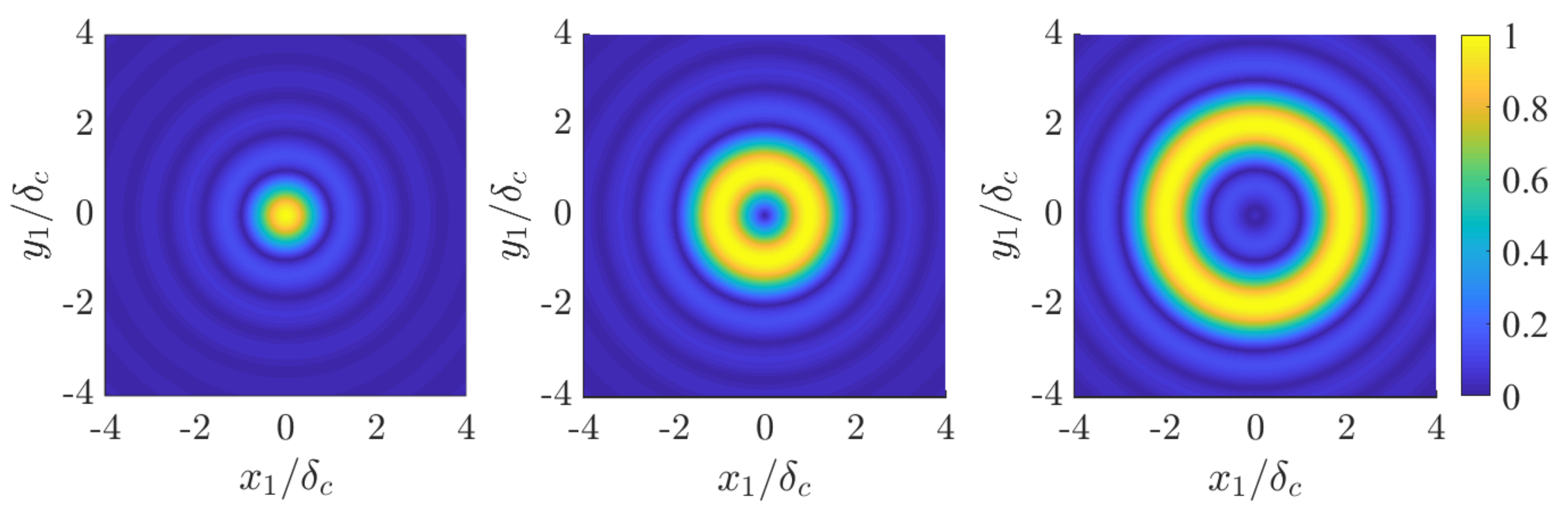
These results are shown in Figure 1, where the absolute value of the degree of coherence between points is plotted as a function of ${\mathbf{r}}_{\mathbf{1}}$ for fixed values of $r_2$. It can be noted that the region where the degree of coherence is significant is a circle for $r_2=0$, but, on increasing $r_2$, becomes a donut (with radius $r_2$). It should be noted that, for a point at a fixed distance $r_2$ from the source center, there is a set of points, located in concentric circles of radius $r_1$, where the field is completely uncorrelated to the field in $r_2$. The radius of these circles satisfies the condition $J_1\left[\zeta (r_2-r_1)/{\delta }_c\right]=0$ with $r_1\ne r_2$.

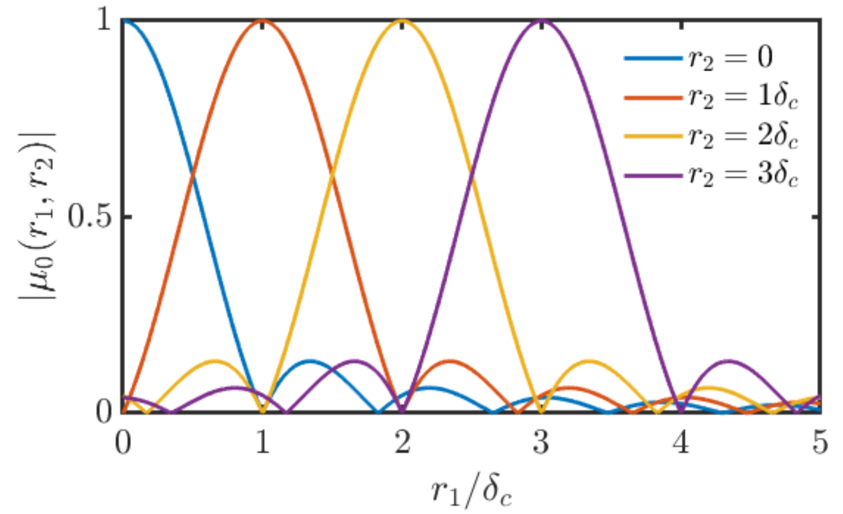
Figure 2 shows the profile of the absolute value of the degree of coherence along a radius $r_1$ for several values of $r_2$. It can be noted that, for $r_2>2{\delta }_c$, the thickness of the donut-shaped area of high coherence is constant, so that the coherence area grows linearly with increasing $r_2$.

Once the function $g\left(r\right)$ has been selected, different sources are obtained on changing the modulating function $\tau \left(\mathbf{r}\right)$. Let us choose $\tau$ as a Laguerre-Gaussian function [29] with Laguerre polynomials of order zero, that is,

$$\begin{array}{c}\hfill \tau \left(\mathbf{r}\right)=\sqrt{I_0}{\left(\frac{\sqrt{2}r}{w_0}\right)}^{m}exp\left(-\frac{r^2}{w_0^2}\right),\end{array}$$

(9)

where $I_0$ is a parameter having dimensions of an irradiance, m is an integer, and $w_0$ is a positive quantity related to the source width. It reduces to a Gaussian function when $m=0$ while, for $m>0$, presents a donut-like shape.The resulting CSD will be denoted by $W_m\left({\mathbf{r}}_1,{\mathbf{r}}_2,0\right)$ and takes the form

$$\begin{array}{c}\hfill W_m\left({\mathbf{r}}_1,{\mathbf{r}}_2,0\right)=I_0{\left(\frac{2r_1{r}_2}{w_0^2}\right)}^{m}exp\left(-\frac{r_1^2+r_2^2}{w_0^2}\right)\frac{2J_1\left[\zeta \left(r_2-r_1\right)/{\delta }_c\right]}{\zeta \left(r_2-r_1\right)/{\delta }_c}.\end{array}$$

(10)

A pseudo-modal expansion in terms of coherent pseudo-modes [27,30] can be written for the whole class of sources described by the CSD of Equation (10) in the following form:

$$W_m\left({\mathbf{r}}_1,{\mathbf{r}}_2,0\right)=I_0\sum _{n=1}^{\infty }{\mathrm{\Lambda }}_{m,n}{\mathrm{\Phi }}_{m,n}\left({\mathbf{r}}_2,0\right){\mathrm{\Phi }}_{m,n}^{*}\left({\mathbf{r}}_1,0\right),$$

(11)

where ${\mathrm{\Lambda }}_{m,n}$ are the pseudo-eigenvalues and the corresponding coherent pseudo-modes are given by

$${\mathrm{\Phi }}_{m,n}\left(\mathbf{r},0\right)=\frac{1}{{\beta }_{m,n}}{\left(\frac{\sqrt{2}r}{w_0}\right)}^{m}exp\left(-\frac{r^2}{w_0^2}\right){\displaystyle \frac{2J_n\left(\zeta r/{\delta }_c\right)}{\zeta r/{\delta }_c}}.$$

(12)

In the derivation of Equation (11), the following relation for the Bessel functions has been taken into account [30,31]:

$${\displaystyle \frac{2J_1\left[\zeta \left(r_2-r_1\right)/{\delta }_c\right]}{\zeta \left(r_2-r_1\right)/{\delta }_c}}=\sum _{n=1}^{\infty }4n^2{\displaystyle \frac{J_n\left(\zeta r_2/{\delta }_c\right)}{\zeta r_2/{\delta }_c}}{\displaystyle \frac{J_n\left(\zeta r_1/{\delta }_c\right)}{\zeta r_1/{\delta }_c}}.$$

(13)

The parameters ${\beta }_{m,n}$ are normalization factors defined as

$${\beta }_{m,n}^2={\int }_0^{\infty }{\int }_0^{2\pi }{\left(\frac{\sqrt{2}r}{w_0}\right)}^{2m}exp\left(-\frac{2r^2}{w_0^2}\right){\left[{\displaystyle \frac{2J_n\left(\zeta r/{\delta }_c\right)}{\zeta r/{\delta }_c}}\right]}^{2}rdrd\theta ,$$

(14)

in such a way that the pseudo-modes ${\mathrm{\Phi }}_{m,n}\left(\mathbf{r},0\right)$ are normalized. However, they are not orthogonal and for this reason we refer to them as pseudo-modes. By comparing Equations (10)–(14), the pseudo-eigenvalues ${\mathrm{\Lambda }}_{m,n}$ can be obtained as ${\mathrm{\Lambda }}_{m,n}=n^2{\beta }_{m,n}^2$ that are explicitly nonnnegative, which confirms the nonnegativeness of the proposed CSD. The normalization factors can be expressed in terms of the generalized hypergeometric functions ${}_p{F}_q\left(a_1,a_2,\cdots ,a_p;b_1,b_2,\cdots ,b_q;c\right)$ [31] as

$${\beta }_{m,n}^2=4\pi {\left(\frac{w_0\zeta }{{\delta }_c}\right)}^{2n}\frac{\left(m+n-1\right)!}{2^{3n}{\left(n!\right)}^2}{}_2{F}_2\left(\frac{1}{2}+n,m+n;1+n,1+2n;-\frac{w_0^2{\zeta }^2}{2{\delta }_c^2}\right).$$

(15)

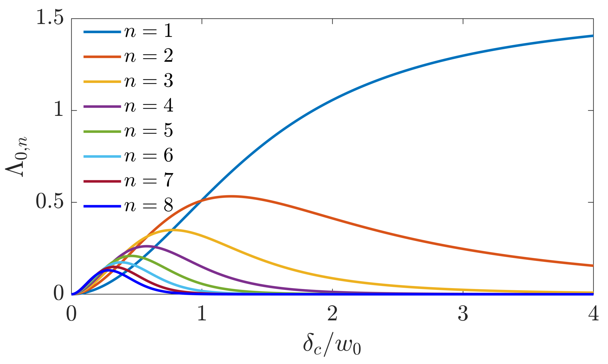
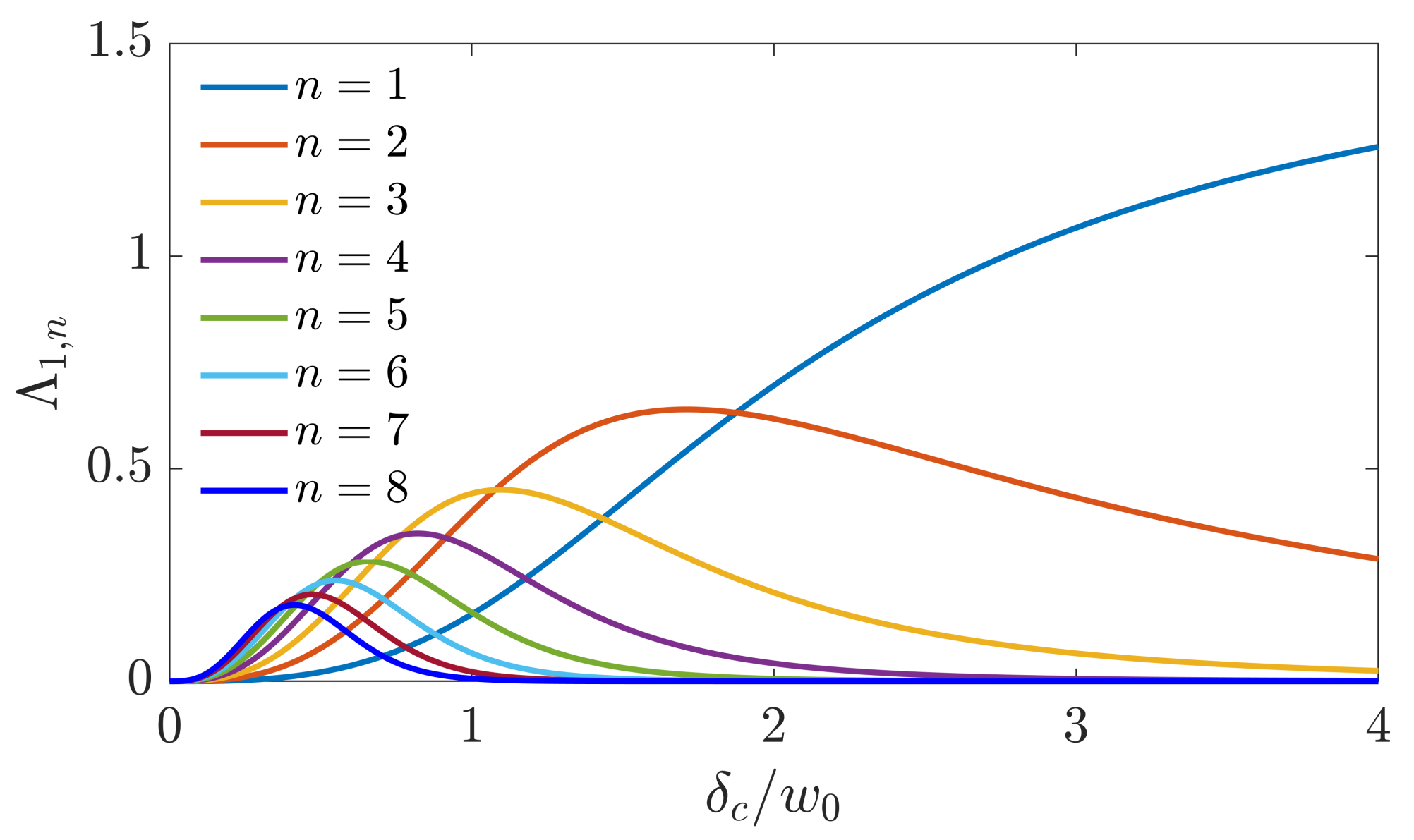
Figure 3 and Figure 4 show the dependence of the first eight pseudo-eigenvalues as functions of the ratio ${\delta }_c/w_0$ for the cases $m=0$ and $m=1$, respectively. It can be observed that, when the value of ${\delta }_c$ is greater than the beam width, the source is almost coherent and can be represented with the contribution of few modes. However, on decreasing the coherence parameter, a larger number of modes is necessary, and this number grows with decreasing ${\delta }_c/w_0$.

It is also seen that the most important contribution for a coherence parameter larger than $w_0$ is due to the lowest-order mode. However, for values of the ratio ${\delta }_c/w_0$ lower than, approximately, 1 (2) for $m=0$ ($m=1$), the first pseudo-eigenvalue is not the highest one, and the contribution of higher-order modes becomes more and more significant for decreasing values of ${\delta }_c/w_0$.

From Figure 3 and Figure 4, it can be concluded that the proposed pseudo-Schell model sources with circular coherence (Equations (3) and (7)) can be synthesized (with the desired precision) just by superposing a sufficiently large number of pseudo-modes with appropriate weights [32,33].

3. Paraxial Propagation

In the following, it will be assumed that the light radiated from the planar source located at the plane $z=0$ propagates under paraxial conditions along the z-axis of a suitable reference frame. The extended Huygens–Fresnel diffraction integral will be used to obtain the CSD of the field at any plane $z=$ constant after propagation through an ABCD optical system as [10]

$$\begin{array}{cc}W\left(\mathbf{R}{}_1,\mathbf{R}{}_2,z\right)\hfill & =\frac{k^2}{4{\pi }^2{B}^2}\int \int W\left(\mathbf{r}{}_1,\mathbf{r}{}_2,0\right)exp\left[-\frac{\mathrm{i}kA}{2B}\left(r_1^2-r_2^2\right)-\frac{\mathrm{i}kD}{2B}\left(R_1^2-R_2^2\right)\right]\hfill \\ & \times exp\left[\frac{\mathrm{i}k}{2B}{r}_1{R}_{1}cos\left({\varphi }_1-{\theta }_1\right)-\frac{\mathrm{i}k}{2B}{r}_2{R}_{2}cos\left({\varphi }_2-{\theta }_2\right)\right]\mathrm{d}{\mathbf{r}}_1\mathrm{d}{\mathbf{r}}_2,\hfill \end{array}$$

(16)

where ${\mathbf{R}}_j=(R_j,{\varphi }_j)$ (with $j=1,2$) are two typical position vectors across the transverse plane $z=$ constant.

For the case of the CSD in Equation (10), the angular integration of Equation (16) gives

$$\begin{array}{cc}{W}_m\left(\mathbf{R}{}_1,\mathbf{R}{}_2,z\right)=\hfill & \frac{I_0{k}^2}{2\pi B^2}exp\left[\frac{\mathrm{i}kD}{2B}\left(R{{}_2}^2-R{{}_1}^2\right)\right]\hfill \\ & \times \underset{0}{\overset{\infty }{\int }}\underset{0}{\overset{\infty }{\int }}{\left(\frac{2r_1{r}_2}{w_0^2}\right)}^{m}exp\left(-\frac{r_1^2+r_2^2}{w_0^2}\right)\frac{2J_1\left[\zeta \left(r_2-r_1\right)/{\delta }_c\right]}{\zeta \left(r_2-r_1\right)/{\delta }_c}\hfill \\ & \times exp\left[\frac{\mathrm{i}kA}{2B}\left(r_2^2-r_1^2\right)\right]J_0\left(\frac{k}{B}{R}_1{r}_1\right)J_0\left(\frac{k}{B}{R}_2{r}_2\right)r_1{r}_2\mathrm{d}{r}_1\mathrm{d}{r}_2,\hfill \end{array}$$

(17)

which allows us to evaluate the irradiance profile and the degree of coherence of the propagated field across any transverse plane.

By choosing the ABCD parameters corresponding to a free space propagation ($A=1$, $B=z$, $C=0$, $D=1$), the evolution of the field CSD can be obtained. Results of the numerical evaluation of Equation (17) are shown in Figure 5 and Figure 6 for $m=0$ and $m=1$, respectively. Both cases present a peculiar behavior of the intensity profile during propagation.

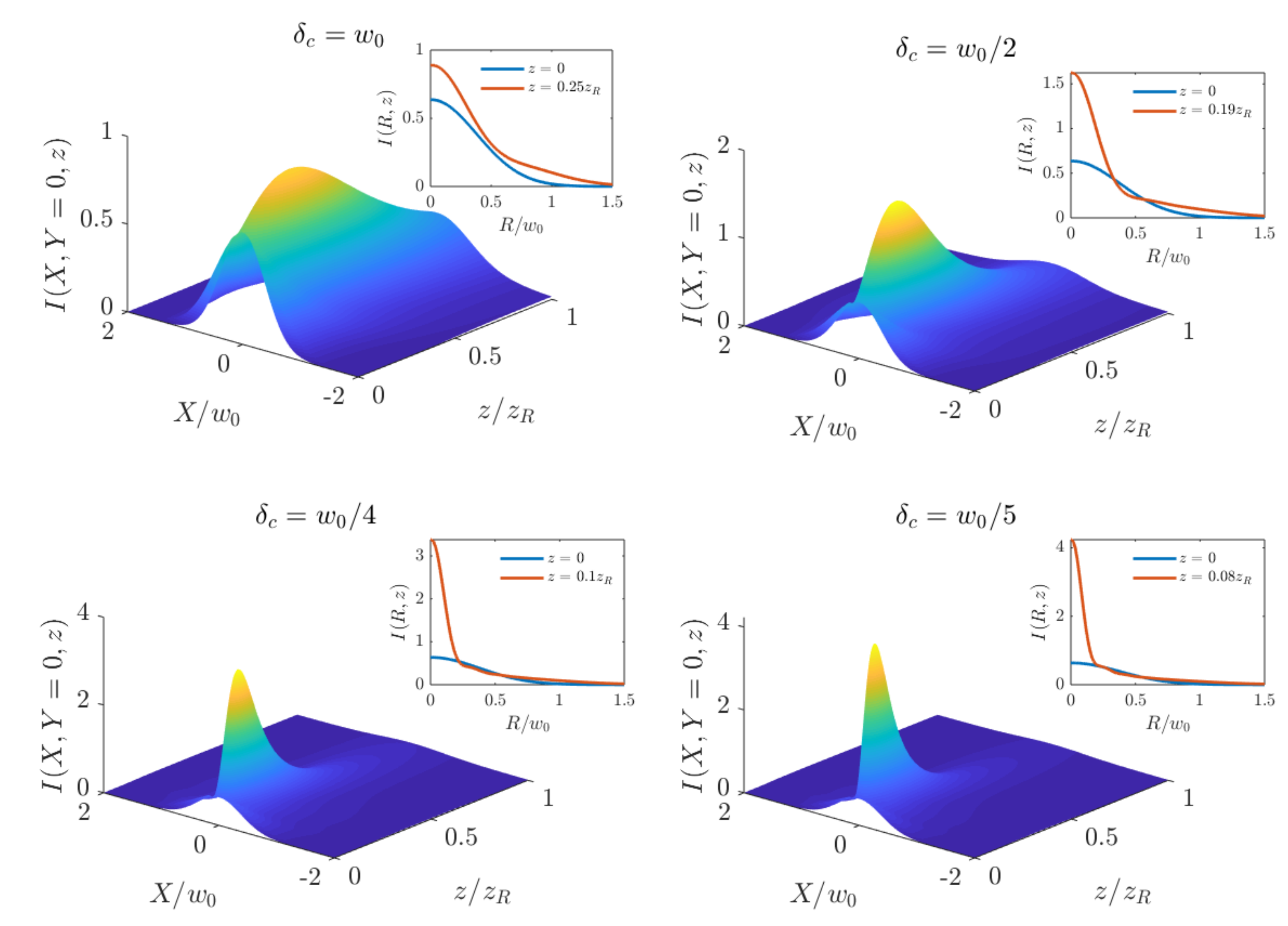
Figure 5 shows the intensity profile for different values of the ratio ${\delta }_c/w_0$ for the case $m=0$. The intensity profile shows a bell-like shape with its peak on the beam axis. It can be observed that, for sufficiently small values of the ratio ${\delta }_c/w_0$, the peak of the intensity profile grows up to a maximum value that is reached at a given propagation distance from the beam waist, which coincides with the source plane. The maximum value of the intensity and the plane at which this maximum is reached depend on the selected value of ${\delta }_c/w_0$. Moreover, the beam shows a sharper intensity profile after a certain propagation distance than at the beam waist, as it can be easily seen from the insets.

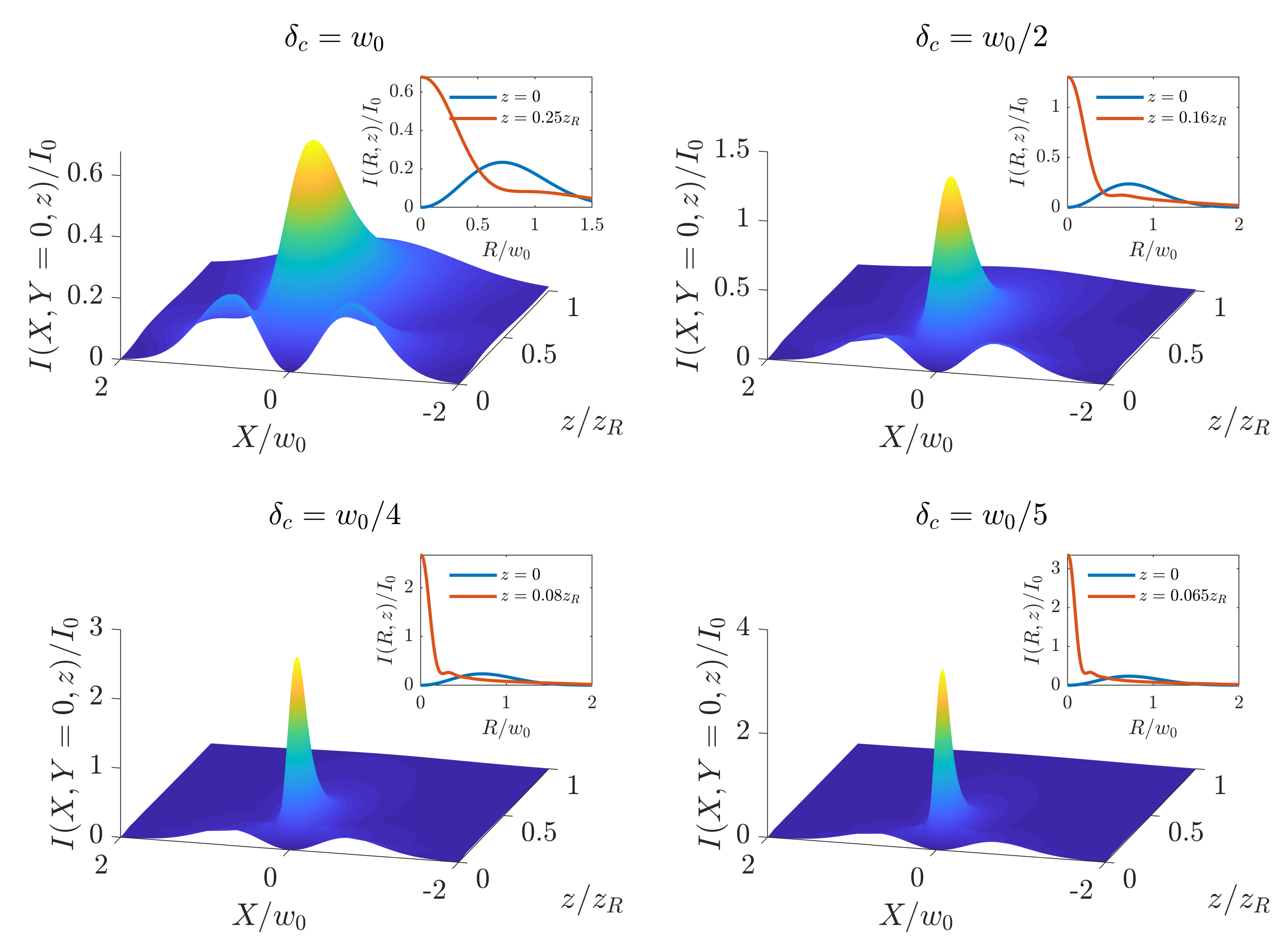
Figure 6 shows the evolution of the intensity profile with the propagation distance for the case $m=1$. At the source plane, the intensity profile shows a donut shape with a zero value at its center (see blue lines in the insets). However, when the beam propagates, the intensity at the beam axis grows and reaches a maximum value at a given propagation distance that depends on the value of the coherence parameter. At the plane where the intensity reaches its maximum, the intensity profile is bell shaped. For lower and lower values of the coherence parameter, a ripple becomes more and more evident (see red lines in the insets). In a similar way that happens for the case with $m=0$, when ${\delta }_c$ is comparable to or lower than $w_0$, the maximum intensity is reached after a certain distance propagation instead of at the source plane. This last fact can be easily observed in the insets of Figure 6, where the intensity profile is drawn for source plane, $z=0$ (blue lines), and for the plane where the maximum intensity is reached (red lines).

4. Trapping Dielectric Nanoparticle with Pseudo-Schell Beams

Previous results suggest that a focused pseudo-Schell model beam could be used for trapping dielectric nanoparticles in a similar way to other kinds of partially coherent beams [5,6,34,35,36,37]. An advantage of the pseudo-Schell model beams is the sharpening of the intensity profile and the high peak that is reached after the source plane (see Figure 5 and Figure 6), which could increase the gradient force exerted on a dielectric particle. By appropriately choosing the source parameters, traps can be obtained with the same beam for particles with a refractive index $n_1$ either higher or lower than the refractive index $n_2$ of the surrounding medium.

If the source plane is at a distance $s_0$ before a thin converging lens with focal length f, the beam propagated at a distance z after the lens focus can be calculated applying Equation (17), where the ABCD transfer matrix has to be chosen as

$$\begin{array}{c}\hfill \left(\begin{array}{cc}A& B\\ C& D\end{array}\right)=\left(\begin{array}{cc}1& f+z\\ 0& 1\end{array}\right)\left(\begin{array}{cc}1& 0\\ -1/f& 1\end{array}\right)\left(\begin{array}{cc}1& s_0\\ 0& 1\end{array}\right)=\left(\begin{array}{cc}-z/f& f+z-z{s}_0/f\\ -1/f& 1-s_0/f\end{array}\right).\end{array}$$

(18)

In the following, we consider a pseudo-Schell model source described by Equation (10) with coherence parameter ${\delta }_c=0.1$ mm, intensity width at the source plane $w_0=0.5$ mm, and $m=1$ (which correspond to the case depicted in the bottom right-hand part of Figure 6). The usual operation line of a visible He–Ne laser is taken for the wavelength $\lambda =632.8$ nm. The source plane is located at $s_0=2.50$ m before a converging lens of focal length $f=5$ mm. These parameters have been chosen to obtain high values of the intensity gradient in a region close to the lens focus, within the paraxial approximation. A factor $I_0=1$ W/mm${}^2$ is taken for calculating the intensity of the generated beam for a propagation distance z after the focus of the lens.

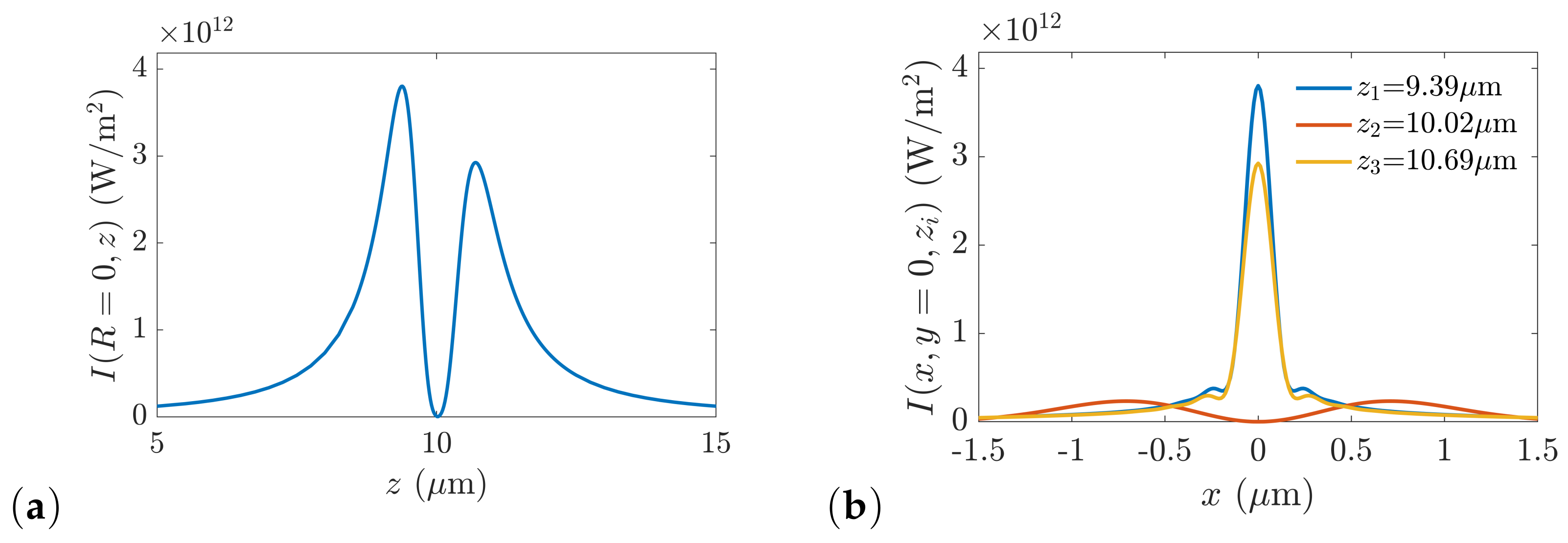
Figure 7a shows the evolution of the intensity at the beam center ($R=0$) along the z-axis in a region after the lens focus. It can be observed that the intensity shows two relative maxima and a relative minimum at given propagation distances in this region. This fast variation of the intensity with propagation distance could be exploited for particle trapping along the z-direction in different positions, depending on the optical properties of the particle. Figure 7b shows the transverse intensity profile of the beam at three different planes, namely, those where the maximum and the minimum axial intensity is reached.

Let us consider a spherical dielectric nanoparticle having a radius smaller than the wavelength of the light ($a<<\lambda$). Therefore, the Rayleigh scattering approximation can be used to obtain the radiation forces exerted on the nanoparticle. Two different contributions can be distinguished: the scattering force and the gradient force.

The first one is directed along the propagation direction and is proportional to the beam intensity. It can be written as [38]

$$\mathbf{F}{}_{\mathrm{Scat}}(X,Y,z)=\frac{8\pi }{3c}{n}_2{\left(ka\right)}^4{a}^2{\left(\frac{n_r^2-1}{n_r^2+2}\right)}^{2}I(X,Y,z)\mathbf{u}{}_{\mathrm{z}},$$

(19)

where c is the speed of light in vacuum, $n_r=n_1/n_2$ is the relative refractive index of the particle, and $\mathbf{u}{}_{\mathrm{z}}$ is a unitary vector along z. The gradient force pushes the particle towards the region of maximum (minimum) intensity if the relative refractive index is higher (lower) than 1. This force can be expressed as [38]

$$\mathbf{F}{}_{\mathrm{Grad}}(X,Y,z)=\frac{2\pi }{c}{n}_2{a}^3\frac{n_r^2-1}{n_r^2+2}\nabla I(X,Y,z).$$

(20)

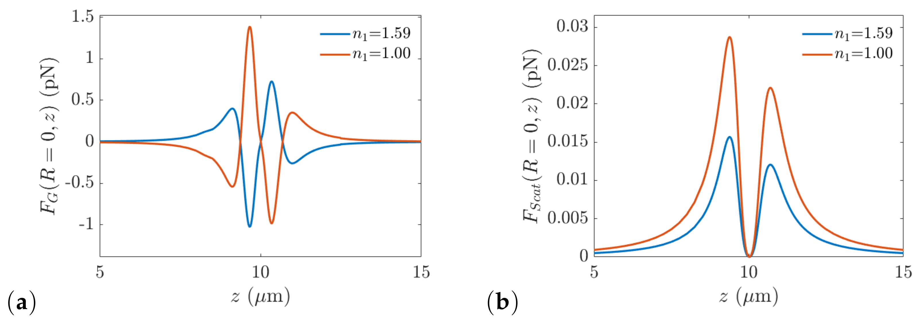
Figure 8a shows the evolution along the beam axis of the z-component of the gradient force on a dielectric nanoparticle with radius $a=30$ nm and refractive index $n_1=1.59$ or $n_1=1.00$ immersed in water ($n_2=1.33$). The on-axis scattering force (that always push the particle away from the focus, $z=0$) is shown in Figure 8b. It must be noted that other forces, such as the weight and buoyancy forces, are of the order of ${10}^{-7}$ pN for dielectric nanoparticles of that size. On the other hand, the Brownian force has a magnitude $F_B=\sqrt{12\pi \kappa a{k}_{B}T}$ [39], where $\kappa$ is the medium viscosity, $k_B$ is the Boltzmann constant and T the temperature. For water at room temperature ($T=300$ K), the viscosity is $\kappa \simeq 7.977\times {10}^{-4}$ Pa, so that the Brownian force is of the order of $2\times {10}^{-3}$ pN. It can be noted that the scattering force is about two orders of magnitude lower than the z-component of the gradient force, so that this is the dominant force, the remaining ones (weight, buoyancy, drag and or Brownian forces) being negligible. Taking these considerations into account, there are two (one) stable equilibrium positions along the z-axis for particles with higher (lower) refractive index than the surrounding medium. These positions correspond to the propagation distances where the on-axis intensity (see Figure 7a) reaches a relative or absolute maximum (minimum) that is, $z_1\simeq 9.39$ $\mathsf{\mu }$m and $z_3\simeq 10.69$ $\mathsf{\mu }$m ($z_2\simeq 10.02$ $\mathsf{\mu }$m).

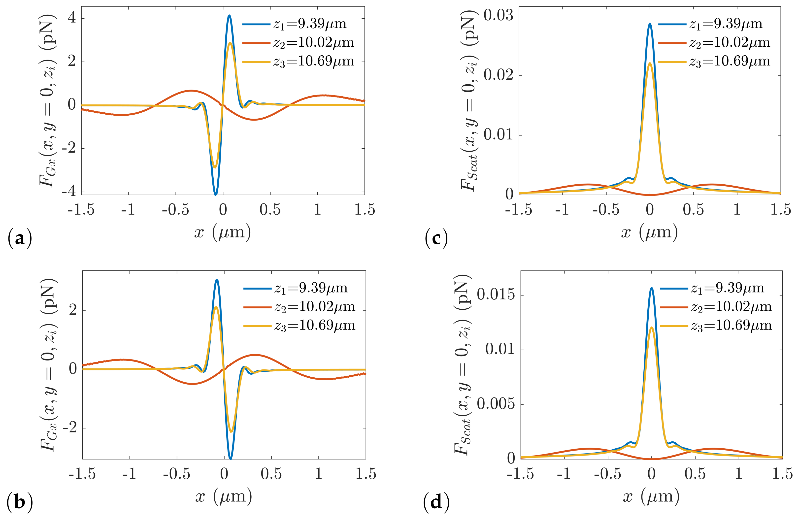
Figure 9 shows the behavior, as functions of the transverse coordinate, of the x-component of the gradient force (parts (a) and (c)) and the scattering force (parts (b) and (d)) at the three planes where a maximum or a minimum of the axial intensity is reached. Due to the circular symmetry of the intensity profile across the transverse section, these results are the same along any radius. Again, the scattering force (always directed along the z-axis) is about two orders of magnitude lower than the gradient force, so that the main effects of the radiation on the particle are due to the gradient force. For the case of dielectric particles with a refractive index lower than that of the surrounding medium (parts (a) and (b) of Figure 9), there is stable equilibrium point in the plane $z_2\simeq 10.02$ $\mathsf{\mu }$nm. In the case of a particle with higher refractive index than the medium (parts (c) and (d) of Figure 9), there is a stable equilibrium point in the plane $z_1\simeq 9.39$ $\mathsf{\mu }$m and another one in the plane $z_3\simeq 10.69$ $\mathsf{\mu }$m.

5. Discussion

Pseudo-Schell model sources present shift invariant coherence properties either along the radial or the angular coordinate. Here, the class of pseudo-Schell model sources with a besinc-like dependence of the coherence on the radial distance (Equation (7)) is analyzed.

Complete coherence is attained for points lying on the same circle, although they can be as far as twice the circle radius. Furthermore, the absolute value of the degree of coherence decreases for pairs of points that belong to circles with greater and greater radii difference, although they can be closer than a pair of points for which complete coherence is found. Complete incoherence is found for points located on different circles with radii difference such that $J_1\left[\zeta (r_2-r_1)/{\delta }_c\right]=0$.

When a Laguerre-Gaussian intensity at the source plane is considered (see Equation (9)), a pseudo-modal expansion [27] of the CSD has been found. Then, these kinds of sources can be synthesized by superposing a large enough number of pseudo-modes [32,33]. Peculiar behavior of the intensity profile with the propagation distance has been found: the profile becomes sharper and the maximum intensity is reached after a propagation distance from the source plane, the latter corresponding to the waist. This effect is more and more evident for lower and lower ratios between the coherence parameter and the beam width. Similar behaviors have been described for other partially coherent beams with nonconventional correlation functions [11,17,20,40,41]

These features could be useful for particle trapping, due to the high intensity gradient that can be obtained along transverse and radial directions on focusing the beam generated by this kind of sources. An example has been developed showing the trapping capabilities of these kinds of beams for nanoparticles presenting a refractive index either higher or lower than the surrounding medium. It should be noted that the trapping of these two types of particles is achieved using the same beam, i.e., a beam generated from a besinc pseudo-Schell source with fixed parameters (${\omega }_0$ and ${\delta }_c$) and a fixed lens.

6. Conclusions

A new class of partially coherent sources, called Besinc Pseudo-Schell Model Sources, has been proposed, for which the degree of coherence across the source plane behaves like $J_1\left[\zeta (r_2-r_1)/{\delta }_c\right]$, $r_1$ and $r_2$ being the radial coordinates of two points. In particular, pairs of points lying on circles concentric to the source center are completely coherent, while they are totally incoherent if $J_1\left[\zeta (r_2-r_1)/{\delta }_c\right]=0$. When a Laguerre-Gaussian intensity profile at the source plane is chosen, the beam radiated from the source has been shown to present a sharp intensity profile within certain propagation ranges, for properly selected source parameters. This effect would allow the simultaneous trapping of dielectric nanoparticles having a refractive index both higher or lower than the surrounding medium by using the same beam. A pseudo-modal expansion for this class of sources has been derived, suggesting a way to experimentally synthesize them.

References

- Ricklin, J.C.; Davidson, F.M. Atmospheric turbulence effects on a partially coherent Gaussian beam: Implications for free-space laser communication. J. Opt. Soc. Am. A 2002, 19, 1794–1802. [Google Scholar] [CrossRef]
- Korotkova, O.; Andrews, L.C.; Phillips, R.L. Model for a partially coherent Gaussian beam in atmospheric turbulence with application in Lasercom. Opt. Eng. 2004, 43, 330–341. [Google Scholar] [CrossRef]
- Gbur, G. Partially coherent beam propagation in atmospheric turbulence [Invited]. J. Opt. Soc. Am. A 2014, 31, 2038–2045. [Google Scholar] [CrossRef] [PubMed] [Green Version]
- Liang, C.; Wu, G.; Wang, F.; Li, W.; Cai, Y.; Ponomarenko, S.A. Overcoming the classical Rayleigh diffraction limit by controlling two-point correlations of partially coherent light sources. Opt. Express 2017, 25, 28352–28362. [Google Scholar] [CrossRef]
- Raghunathan, S.B.; van Dijk, T.; Peterman, E.J.G.; Visser, T.D. Experimental demonstration of an intensity minimum at the focus of a laser beam created by spatial coherence: Application to the optical trapping of dielectric particles. Opt. Lett. 2010, 35, 4166–4168. [Google Scholar] [CrossRef] [PubMed]
- Zhao, C.; Cai, Y. Trapping two types of particles using a focused partially coherent elegant Laguerre– Gaussian beam. Opt. Lett. 2011, 36, 2251–2253. [Google Scholar] [CrossRef] [PubMed]
- Korotkova, O. Random Light Beams: Theory and Applications; CRC Press Taylor & Francis Group: Boca Raton, FL, USA, 2014. [Google Scholar]
- Cai, Y.; Chen, Y.; Yu, J.; Liu, X.; Liu, L. Generation of Partially Coherent Beams. Prog. Opt. 2017, 62, 157–223. [Google Scholar] [CrossRef]
- Schell, A. A technique for the determination of the radiation pattern of a partially coherent aperture. IEEE Trans. Antennas Propag. 1967, 15, 187–188. [Google Scholar] [CrossRef]
- Mandel, L.; Wolf, E. Optical Coherence and Quantum Optics; Cambridge University Press: Cambridge, UK, 1995. [Google Scholar]
- Lajunen, H.; Saastamoinen, T. Propagation characteristics of partially coherent beams with spatially varying correlations. Opt. Lett. 2011, 36, 4104–4106. [Google Scholar] [CrossRef]
- Mei, Z.; Korotkova, O. Random sources generating ring-shaped beams. Opt. Lett. 2013, 38, 91–93. [Google Scholar] [CrossRef]
- Santarsiero, M.; Piquero, G.; de Sande, J.C.G.; Gori, F. Difference of cross-spectral densities. Opt. Lett. 2014, 39, 1713–1716. [Google Scholar] [CrossRef] [PubMed]
- De Sande, J.C.G.; Santarsiero, M.; Piquero, G.; Gori, F. The subtraction of mutually displaced Gaussian Schell-model beams. J. Opt. 2015, 17, 125613. [Google Scholar] [CrossRef]
- Santarsiero, M.; Martínez-Herrero, R.; Maluenda, D.; de Sande, J.C.G.; Piquero, G.; Gori, F. Partially coherent sources with circular coherence. Opt. Lett. 2017, 42, 1512–1515. [Google Scholar] [CrossRef] [PubMed] [Green Version]
- Santarsiero, M.; Martínez-Herrero, R.; Maluenda, D.; de Sande, J.C.G.; Piquero, G.; Gori, F. Synthesis of circularly coherent sources. Opt. Lett. 2017, 42, 4115–4118. [Google Scholar] [CrossRef] [PubMed]
- Wu, D.; Wang, F.; Cai, Y. High-order nonuniformly correlated beams. Opt. Laser Technol. 2018, 99, 230–237. [Google Scholar] [CrossRef]
- Piquero, G.; Santarsiero, M.; Martínez-Herrero, R.; de Sande, J.C.G.; Alonzo, M.; Gori, F. Partially coherent sources with radial coherence. Opt. Lett. 2018, 43, 2376–2379. [Google Scholar] [CrossRef] [PubMed]
- Hyde, M. Controlling the Spatial Coherence of an Optical Source Using a Spatial Filter. Appl. Sci. 2018, 8, 1465. [Google Scholar] [CrossRef]
- De Sande, J.C.G.; Martínez-Herrero, R.; Piquero, G.; Santarsiero, M.; Gori, F. Pseudo-Schell model sources. Opt. Express 2019, 27, 3963–3977. [Google Scholar] [CrossRef]
- Ma, P.; Kacerovská, B.; Khosravi, R.; Liang, C.; Zeng, J.; Peng, X.; Mi, C.; Monfared, Y.E.; Zhang, Y.; Wang, F.; et al. Numerical Approach for Studying the Evolution of the Degrees of Coherence of Partially Coherent Beams Propagation through an ABCD Optical System. Appl. Sci. 2019, 9, 2084. [Google Scholar] [CrossRef]
- Liang, C.; Khosrav, R.; Liang, X.; Kacerovská, B.; Monfared, Y.E. Standard and elegant higher-order Laguerre-Gaussian correlated Schell-model beams. J. Opt. 2019. [Google Scholar] [CrossRef]
- Zhang, M.; Liu, X.; Guo, L.; Liu, L.; Cai, Y. Partially Coherent Flat-Topped Beam Generated by an Axicon. Appl. Sci. 2019, 9, 1499. [Google Scholar] [CrossRef]
- Martínez-Herrero, R.; Maluenda, D.; Piquero, G.; de Sande, J.C.G. Vortex pseudo Schell-model source: A proposal. In Proceedings of the 2016 15th Workshop on Information Optics (WIO), Barcelona, Spain, 11–15 July 2016; pp. 1–3. [Google Scholar] [CrossRef]
- Martínez-Herrero, R.; de Sande, J.C.G.; Piquero, G.; Santarsiero, M.; Alonzo, M.; Gori, F. Sources with radial and circular coherence. In Proceedings of the 2nd Joensuu Conference on Coherence and Random Polarization, Trends in Electromagnetic Coherence, Joensuu, Finland, 12–15 June 2018; pp. 114–115. [Google Scholar]
- Gori, F.; Santarsiero, M. Devising genuine spatial correlation functions. Opt. Lett. 2007, 32, 3531–3533. [Google Scholar] [CrossRef] [PubMed] [Green Version]
- Martínez-Herrero, R.; Mejías, P.M.; Gori, F. Genuine cross-spectral densities and pseudo-modal expansions. Opt. Lett. 2009, 34, 1399–1401. [Google Scholar] [CrossRef] [PubMed]
- Abramowitz, M.; Stegun, I. (Eds.) Handbook of Mathematical Functions; Dover Publications Inc.: Mineola, NY, USA, 1972. [Google Scholar]
- Siegman, A.E. Lasers; University Science Books: Sausalito, CA, USA, 1986. [Google Scholar]
- Yang, S.; Ponomarenko, S.A.; Chen, Z.D. Coherent pseudo–mode decomposition of a new partially coherent source class. Opt. Lett. 2015, 40, 3081–3084. [Google Scholar] [CrossRef] [PubMed]
- Prudnikov, A.; Brychkov, I.; Brychkov, I.; Marichev, O. Integrals and Series: Special Functions; Gordon and Breach Science Publishers: New York, NY, USA, 1986. [Google Scholar]
- Rodenburg, B.; Mirhosseini, M.; Magaña-Loaiza, O.S.; Boyd, R.W. Experimental generation of an optical field with arbitrary spatial coherence properties. J. Opt. Soc. Am. B 2014, 31, A51–A55. [Google Scholar] [CrossRef] [Green Version]
- Chen, X.; Li, J.; Rafsanjani, S.M.H.; Korotkova, O. Synthesis of Im-Bessel correlated beams via coherent modes. Opt. Lett. 2018, 43, 3590–3593. [Google Scholar] [CrossRef] [PubMed]
- Zhou, Y.; Xu, H.; Yuan, Y.; Peng, J.; Qu, J.; Huang, W. Trapping Two Types of Particles Using a Laguerre–Gaussian Correlated Schell-Model Beam. IEEE Photonics J. 2016, 8, 6600710. [Google Scholar] [CrossRef]
- Jiang, Y.; Cao, Z.; Shao, H.; Zheng, W.; Zeng, B.; Lu, X. Trapping two types of particles by modified circular Airy beams. Opt. Express 2016, 24, 18072–18081. [Google Scholar] [CrossRef]
- Zhang, H.; Li, J.; Cheng, K.; Duan, M.; Feng, Z. Trapping two types of particles using a focused partially coherent circular edge dislocations beam. Opt. Laser Technol. 2017, 97, 191–197. [Google Scholar] [CrossRef]
- Duan, M.; Zhang, H.; Li, J.; Cheng, K.; Wang, G.; Yang, W. Trapping two types of particles using a focused partially coherent modified Bessel-Gaussian beam. Opt. Lasers Eng. 2018, 110, 308–314. [Google Scholar] [CrossRef]
- Harada, Y.; Asakura, T. Radiation forces on a dielectric sphere in the Rayleigh scattering regime. Opt. Commun. 1996, 124, 529–541. [Google Scholar] [CrossRef]
- Okamoto, K.; Kawata, S. Radiation Force Exerted on Subwavelength Particles near a Nanoaperture. Phys. Rev. Lett. 1999, 83, 4534–4537. [Google Scholar] [CrossRef]
- Cai, Y.; Chen, Y.; Wang, F. Generation and propagation of partially coherent beams with nonconventional correlation functions: A review [Invited]. J. Opt. Soc. Am. A 2014, 31, 2083–2096. [Google Scholar] [CrossRef] [PubMed]
- Ding, C.; Koivurova, M.; Turunen, J.; Pan, L. Self-focusing of a partially coherent beam with circular coherence. J. Opt. Soc. Am. A 2017, 34, 1441–1447. [Google Scholar] [CrossRef] [PubMed]
Figure 1.
Absolute value of the degree of coherence relative to a point located at the following distances from the source center: (left); (center), and (right).
Figure 2.
Absolute value of the degree of coherence as a function of the radius for different distances from the source center.
Figure 3.
Pseudo-eigenvalues, , for the CSD in Equation (10) with as functions of the ratio . The values of are evaluated from Equation (15).
Figure 4.
Figure 5.
Evolution of the intensity profile with propagation distance for a beam with and different values of the ratio [numerical evaluation of Equation (17) for free space propagation]. The insets show the intensity profile across the source plane and across the plane where the maximum intensity is reached.
Figure 6.
Figure 7.
(a) evolution of the intensity in the beam axis with propagation distance after the focus of a lens and (b) intensity profile at different propagation distances for a source with , nm, mm and mm. Other parameters are mm, m, and W/mm.
Figure 8.
(a) z-component of the gradient force and (b) scattering force along the beam axis for a dielectric nanoparticle with radius nm and having a refractive index higher (blue line) or lower (red line) than that of the surrounding medium (). Other parameters are the same as in Figure 7.
Figure 9.
(a) x-component of the gradient force for and (b) for , and (c) scattering force for and (d) for . In all cases, . Other parameters are the same as in Figure 7.
© 2019 by the authors. Licensee MDPI, Basel, Switzerland. This article is an open access article distributed under the terms and conditions of the Creative Commons Attribution (CC BY) license (http://creativecommons.org/licenses/by/4.0/).
Share and Cite
MDPI and ACS Style
Martínez-Herrero, R.; Piquero, G.; González de Sande, J.C.; Santarsiero, M.; Gori, F. Besinc Pseudo-Schell Model Sources with Circular Coherence. Appl. Sci. 2019, 9, 2716. https://0-doi-org.brum.beds.ac.uk/10.3390/app9132716
AMA Style
Martínez-Herrero R, Piquero G, González de Sande JC, Santarsiero M, Gori F. Besinc Pseudo-Schell Model Sources with Circular Coherence. Applied Sciences. 2019; 9(13):2716. https://0-doi-org.brum.beds.ac.uk/10.3390/app9132716
Chicago/Turabian StyleMartínez-Herrero, Rosario, Gemma Piquero, Juan Carlos González de Sande, Massimo Santarsiero, and Franco Gori. 2019. "Besinc Pseudo-Schell Model Sources with Circular Coherence" Applied Sciences 9, no. 13: 2716. https://0-doi-org.brum.beds.ac.uk/10.3390/app9132716
Note that from the first issue of 2016, this journal uses article numbers instead of page numbers. See further details here.