Automatic Bridge Crack Detection Using a Convolutional Neural Network


School of Precision Instruments and Optoelectronics Engineering, Tianjin University, 300072 Tianjin, China
*
Author to whom correspondence should be addressed.
Appl. Sci. 2019, 9(14), 2867; https://0-doi-org.brum.beds.ac.uk/10.3390/app9142867
Submission received: 14 June 2019
/
Revised: 4 July 2019
/
Accepted: 4 July 2019
/
Published: 18 July 2019
Abstract
:Concrete bridge crack detection is critical to guaranteeing transportation safety. The introduction of deep learning technology makes it possible to automatically and accurately detect cracks in bridges. We proposed an end-to-end crack detection model based on the convolutional neural network (CNN), taking the advantage of atrous convolution, Atrous Spatial Pyramid Pooling (ASPP) module and depthwise separable convolution. The atrous convolution obtains a larger receptive field without reducing the resolution. The ASPP module enables the network to extract multi-scale context information, while the depthwise separable convolution reduces computational complexity. The proposed model achieved a detection accuracy of 96.37% without pre-training. Experiments showed that, compared with traditional classification models, the proposed model has a better performance. Besides, the proposed model can be embedded in any convolutional network as an effective feature extraction structure.
1. Introduction
Bridges play a significant role in daily life. Regular bridge checks are important for maintaining the structural health and reliability of bridges. Bridge crack is one of the main damages of bridges, and its detection is an important task for bridge maintenance. Traditional bridge detection methods rely on human visual inspection, so the detection efficiency and accuracy cannot be guaranteed. In recent years, machine learning and computer vision were applied to the field of crack detection [1,2,3,4,5], and achieved good results.
The modern convolutional neural network (CNN) was first proposed by LeCun et al. [6] in 1989. Due to its effectiveness in feature extraction, it is widely used in computer vision tasks such as image classification [7,8,9,10], object recognition [11,12,13], and action recognition [14,15,16].
Inspired by these achievements, recent studies have applied convolutional neural networks to the area of crack detection. In 2004, Ouellette et al. [17] introduced an algorithm, based on the standard genetic algorithm (GA), to automatically detect cracks, which had a crack detection accuracy of 92.3 ± 1.4% for 100 images. Since the dataset was too small, the effectiveness of this method cannot be fully proven. In 2016, Zhang [18] et al. proposed an algorithm for classifying pavement cracks. However, since the algorithm did not have strict classification criteria for positive and negative samples, the detection accuracy was only 86.96%. In 2017, based on transfer learning, Gopalakrishnan et al. [19] proposed a concrete crack classifier, where the Visual Geometry Group Network 16(VGG-16) model got the best performance. In the same year, an algorithm for analyzing cracks in a single video frame using a convolutional neural network was developed by Chen et al. [20], combined with the Naïve Bayes data fusion scheme to aggregate video information. The network trained by Cha et al. [21], combined with the sliding window technique, could scan any particular crack image with a resolution larger than 256 × 256 pixels. Wang et al. [22] used CNN to detect pavement cracks and used principal component analysis (PCA) to classify the detected pavement cracks. Pauly et al. [23] demonstrated the effectiveness of using deeper networks to improve the detection accuracy in computer vision-based pavement crack detection. However, these methods still have problems of low precision or high model complexity, so they are not widely used.
In this article, we proposed an end-to-end model based on the convolutional neural network to detect bridge cracks automatically. Our main contributions are as follows:
- We used a single CNN trained end-to-end with images to detect cracks, using only images and image labels as input. Our CNN model achieved a 96.37% accuracy in detecting cracks without pre-training and fine-tuning on other datasets.
- To the best of our knowledge, we introduced the Atrous Spatial Pyramid Pooling (ASPP) module into the field of crack detection for the first time, and achieved good experimental results.
- We introduced atrous convolution with an atrous rate of 2 in the last three convolutional layers of the network, replacing the maxpooling layer, and thus avoiding the loss of crack edge information caused by pooling. We proved the effectiveness of replacing the maxpooling layer with atrous convolution through experiments.
2. Materials and Methods
2.1. Datasets
According to [24], there is currently no unified bridge crack database published. Therefore, in order to meet the experimental requirements, the bridge crack dataset in [24] is artificially augmented to generate the dataset used in this paper. In order to promote the development of crack detection algorithms, we share our dataset on https://github.com/tjdxxhy/crack-detection.
The original dataset is composed of 2068 bridge crack images collected by the Phantom 4 Pro’s CMOS surface array camera with a resolution of 1024 × 1024. The bridge crack dataset we used was generated by the original dataset through the following operations:
- Data preprocessing: Since the pictures in the original dataset all contain cracks, which were not conducive to the differentiation of positive and negative samples during network training, we cropped a 1024 × 1024 resolution image into four 512 × 512 resolution images. Then, the obtained 8272 pictures were filtered to remove the blurred pictures, and a crack dataset containing 6069 images was obtained. The dataset included 4058 crack images and 2011 background images, with the ratio of crack images to background images being about 2:1. At last, we randomly selected 4856 images as the training set and 1213 images as the testing set.
- Data augmentation: In order to meet the input requirements of the network, we cropped the picture size to 224 × 224 through the random center crop operation. Then, we randomly flipped the training set images to further augment the dataset.
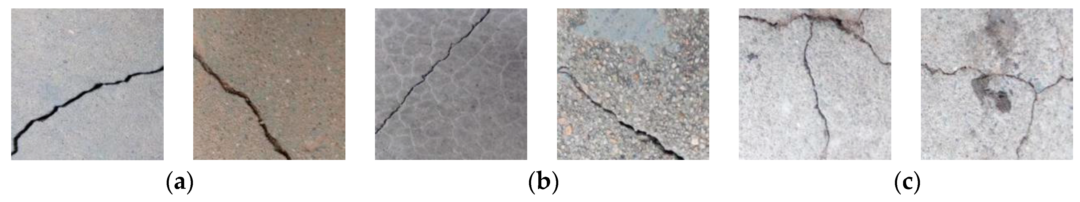
Some examples of images in our dataset are shown in Figure 1. To create a robust crack classifier, in addition to good images(1(a)), our dataset also contains images of bridge shading(1(b)), water stains, and strong light(1(c)).
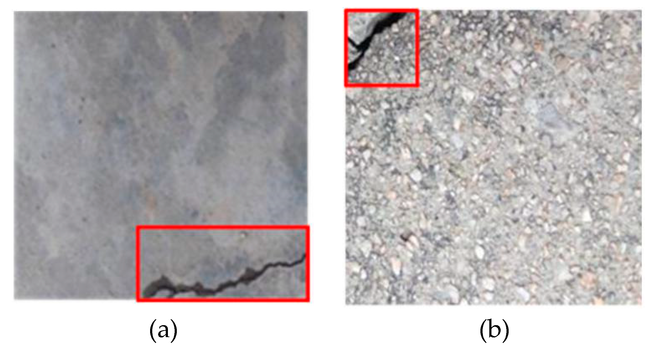
There are some images containing cracks in edges in our cropped dataset, as shown in Figure 2. Having these images in the dataset has the following advantages: (1) In these images, the cracks only occupy a small proportion of the image. After the CNN operation, the feature map will become smaller. If our model can successfully distinguish the cracks in such images, it is proved that our model can effectively extract the deep characteristics of the cracks. (2) In the actual application, the proportion of cracks in the image is small, so the inclusion of these images can increase the practicality of the proposed model.
2.2. Proposed Model
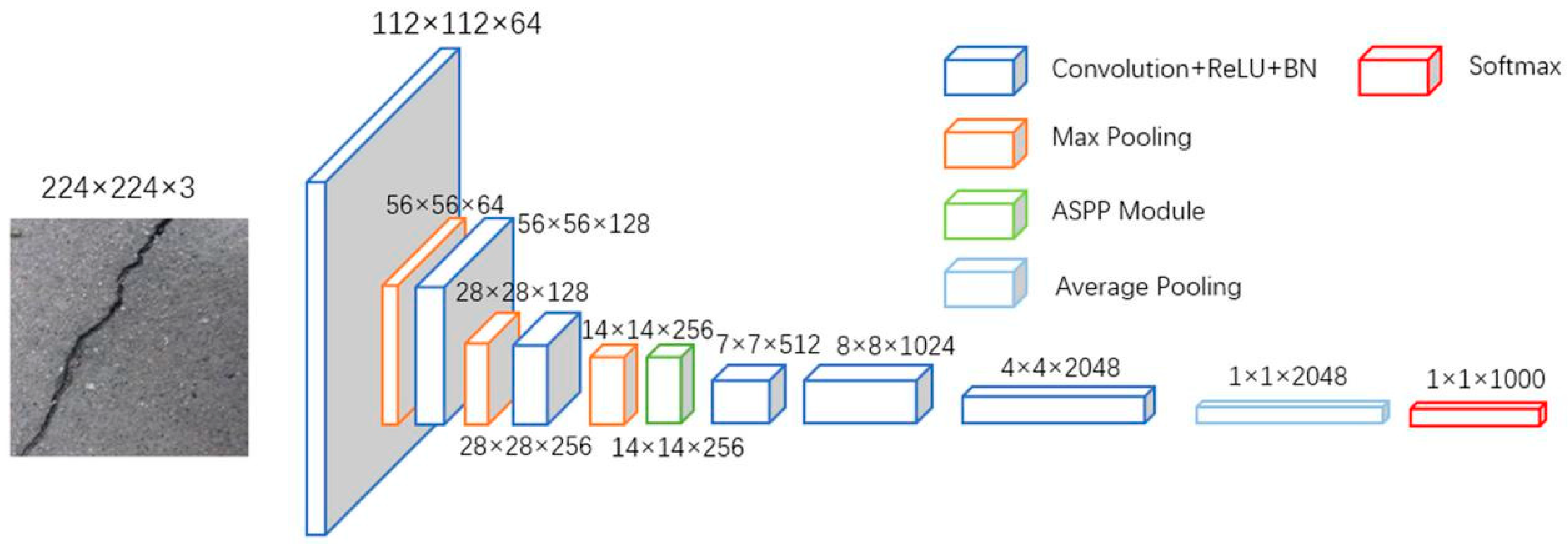
The end-to-end CNN model proposed in this paper is shown in Figure 3. The network contains a total of 28 layers, including 16 convolutional layers and 3 maxpooling layers, while the Atrous Spatial Pyramid Pooling (ASPP) module contains 10 convolutional layers. In the structure shown in Figure 3, the first three convolutional layers are used to extract image features, and the output feature maps are then input into the ASPP module, whose structure will be described in detail in Section 2.2.3, to extract the multi-scale crack feature information. Furthermore, the depthwise separable convolution contained in the ASPP module reduces the computational complexity of the model, thus making the network easier to optimize. In the last three convolutional layers of the network, we apply atrous convolution to replace the maxpooling layers, thus avoiding the degradation of the image resolution while increasing the receptive field. At last, the network uses Softmax to classify the input pictures (cracks or backgrounds).
2.2.1. Atrous Convolution
Modern image classification networks integrate multi-scale context information through continuous pooling and down-sampling layers, resulting in a loss of detail information about the object edges and a degradation of the image resolution [25,26]. To solve this problem, Yu et al. [27] proposed a novel convolution method—atrous convolution (also called dilated convolution). Atrous convolution can exponentially expand the receptive field without a loss of resolution, resulting in a denser feature map [27].
Let denotes a discrete function. Let and be a discrete filter of size . Then, the discrete convolution operator can be defined as:
We now promote this operator. Let be an atrous factor, and let be defined as:
Here, is the atrous convolution or l-atrous convolution. The discrete convolution we are familiar with is an atrous convolution of .
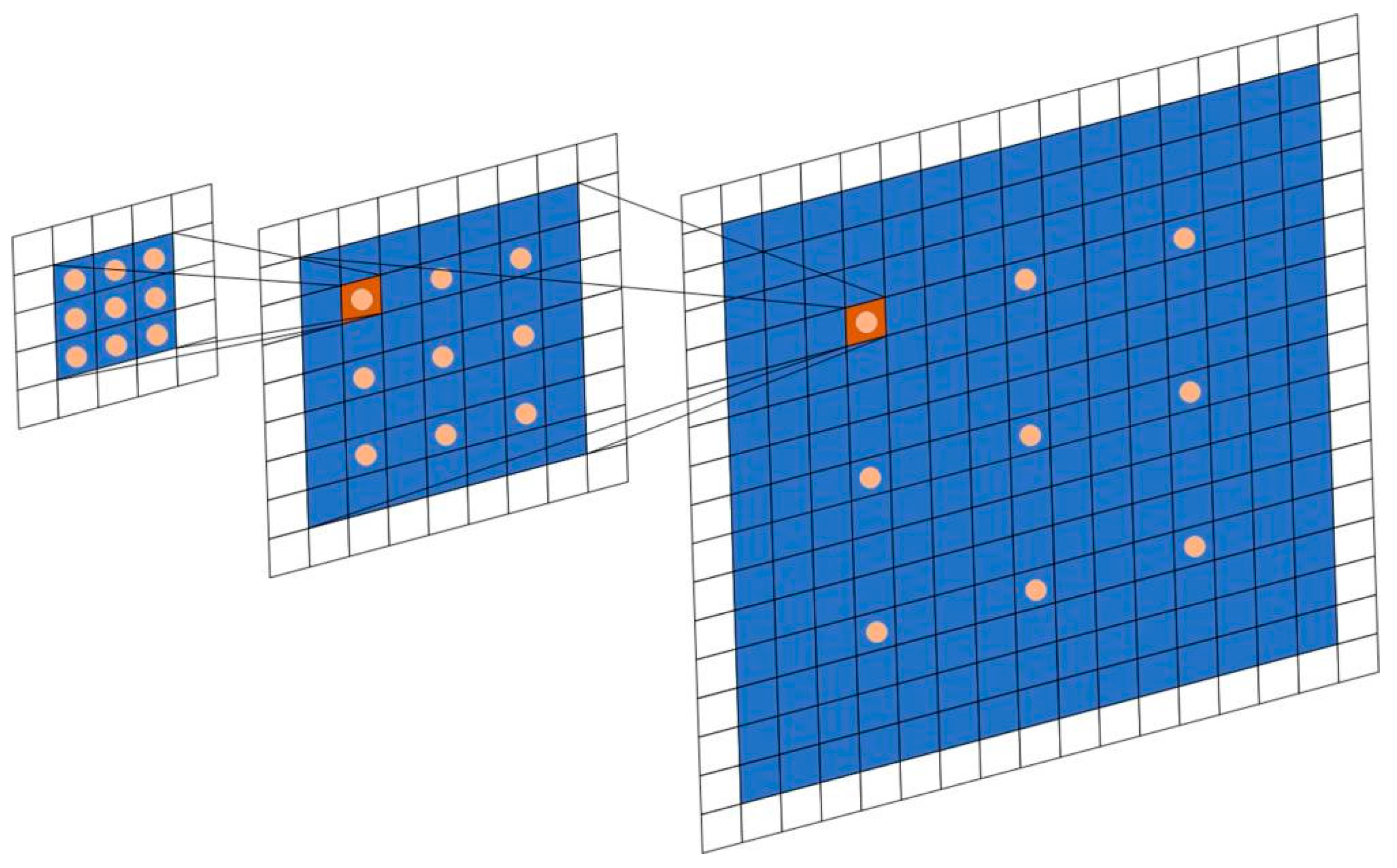
Atrous convolution enables an exponential expansion of the receptive field without a loss of resolution and coverage [27]. Let be discrete functions, and let be discrete 3 × 3 filters. Consider applying an atrous filter with an exponential increase:
The receptive field of the element p in is defined as the set of elements in that modify the value of . Assume that the size of the receptive field of p in is the number of these elements. Then, the receptive field size of each element in is . The receptive field is an exponentially increasing square, as shown in Figure 4.
In our crack detection task, special attention was paid to the edge and texture information of the crack. However, continuous pooling and down-sampling layers will result in the loss of the object edge detail information and a reduced image resolution [25,26]. For example, after four pooling layers, the information of any object smaller than 16 pixels would be lost. In the last few layers of the network, the resolution of the feature map is small, so using the atrous convolution instead of the maxpooling layer can effectively preserve the resolution of the feature map and provide more feature information for the final classification, thereby obtaining a higher accuracy. Therefore, atrous convolution with an atrous rate of 2 was introduced in the last three convolutional layers of the network. As a result, the loss of edge detail information or the reduction of the image resolution is avoided, while a larger receptive field is obtained.
2.2.2. Depthwise Separable Convolution
The depthwise separable convolution was originally proposed by Laurent Sifre [28]. After that, it was widely known and applied in models such as Inception [29], Xception [30], and MobileNets [31].
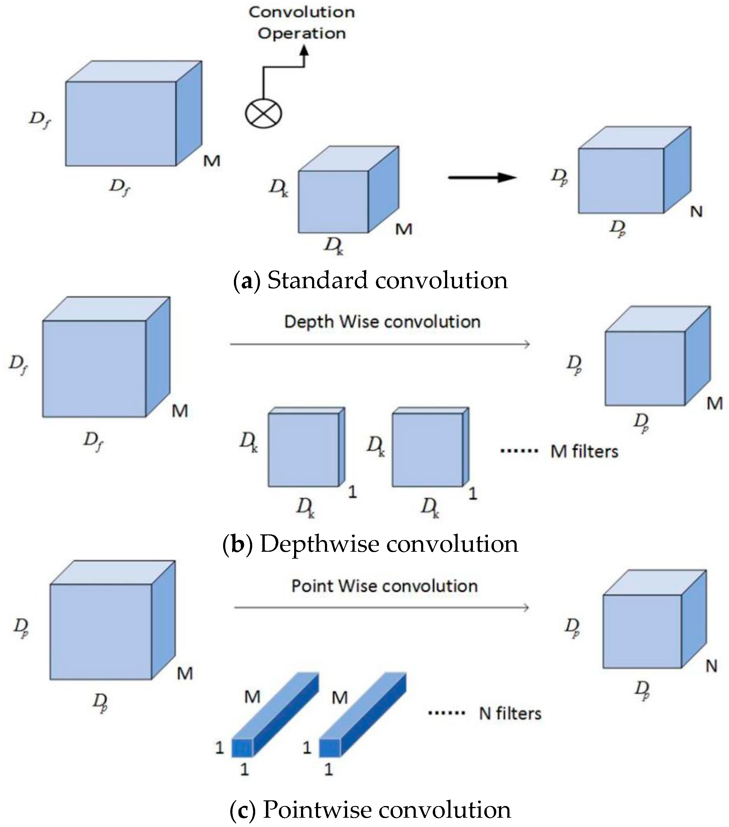
The depthwise separable convolution resolves the standard convolution into a depthwise convolution and a pointwise convolution. The spatial depthwise convolution is used independently on each channel of the input feature map, and then the outputs of the depthwise convolution are combined using a pointwise convolution. The Depthwise separable convolution can greatly reduce the model parameters and computational complexity, while maintaining a similar or better performance [32]. Figure 5 shows how the standard convolution (Figure 5a) is decomposed into a depthwise convolution (Figure 5b) and a 1 × 1 pointwise convolution (Figure 5c).
The standard convolutional layer takes the feature map F of size as an input and produces a feature map G of size , where is the spatial width and height of the input square feature map, M is the number of input channels, is the spatial width and height of the output square feature map, and N is the number of output channels [31].
The standard convolutional layer is convolved by a convolution kernel K of size , where is the spatial width and height of the convolution kernel (which is assumed to be squared), M is the number of input channels, and N is the number of output channels.
The calculation cost of the standard convolution is shown in Equation (4):
In Equation (4), the computational cost of the standard convolution increases exponentially with the output feature map size and the convolution kernel size , the number of input channels M, and the number of output channels N.
The depthwise separable convolution integrates the traditional convolution into two layers; the first layer is the filter layer, and the spatial convolution is performed on each channel of the input feature map by a depthwise convolution; the second layer is the combined layer, using a 1 × 1 pointwise convolution to combine the outputs of the depthwise convolution.
The computational cost of the depthwise convolution is shown in Equation (5):
The computational cost of the 1 × 1 pointwise convolution is shown in Equation (6):
The computational cost of the depthwise separable convolution is shown in Equation (7), which is the sum of the depthwise convolution and the pointwise convolution:
By decomposing the standard convolution into the filter layer and the combined layer, we get a reduction in the amount of computation, as shown in Equation (8):
The standard convolution simultaneously learns spatial information and the correlation between channels, while the depthwise separable convolution first performs a depthwise convolution, broadens the network so that it can extract more network features, and then performs a 1 × 1 pointwise convolution, by which the outputs of the depthwise convolution are linearly combined to generate new features. Compared to the traditional convolution, the computational amount and model complexity of the depthwise separable convolution are greatly reduced, making it a more efficient convolution method that is able to be used to learn representative features better with less data. These advantages of the depthwise separable convolution structure are especially important for our crack detection model: our task is to train the model from scratch on a crack dataset, and the depthwise separable convolution allows us to learn the full feature representation of the data efficiently, thereby improving the model’s cracks detection performance.
2.2.3. ASPP Module
In deep neural networks, the size of the receptive field can roughly indicate the extent to which context information is used [33]. However, Zhou et al. [34] proved that the empirical receptive field of CNN was much smaller than the theoretical receptive field, especially in the higher layers. This greatly limits the ability of CNN to use context information to get accurate predictions. Global average pooling [35] is an effective method to obtain global context information, and has been applied in image classification tasks [29,36] to solve the above problem.
However, directly fusing the information obtained by global averaging pooling to form a single vector may result in loss of sub-region context information [33]. He, K et al. [37] proposed a layered Spatial Pyramid Pooling (SPP), which can obtain the fusion of information and receptive fields from different sub-regions. Experiments show that multi-scale feature information fusion will bring about the improvement of network accuracy. This is not simply because of the increase in parameters, but because multi-level pooling can effectively deal with object deformation and differences in the spatial layout [38].
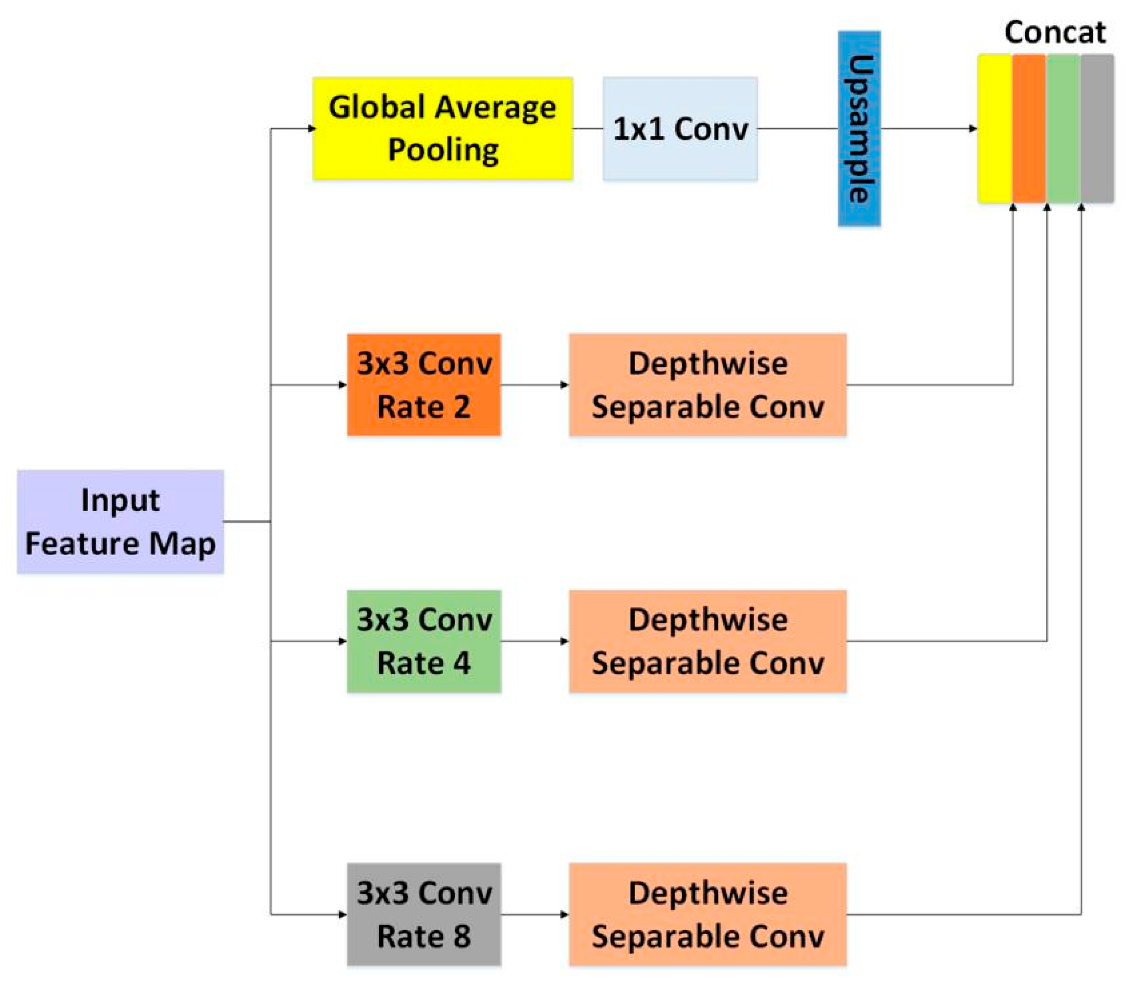
For bridge crack pictures, cracks usually only occupy a small part of the picture. Therefore, in order to accurately identify cracks, it is necessary to effectively utilize context information and accurately extract crack features. Compared with the SPP structure in [37], the atrous convolution used by the ASPP structure avoids the loss of image detail information caused by the down-sampling operation; therefore, it fits better with the need to detect cracks. Consequently, the ASPP module is introduced in the network, and it is part of the DeepLabv2 [39] network proposed by the Google team in 2017. It performs parallel atrous sampling at different sample rates on a given input, which is equivalent to capturing the context of an image in multiple scales, thereby obtaining multi-scale image feature information [32].
The structure of the ASPP module we used is shown in Figure 6. On the feature map extracted by the first few layers of CNN in Figure 3, the atrous convolutions with rates of 2, 4, and 8 were performed in parallel, and the feature maps extracted for each atrous rate were further processed by a depthwise separable convolution in a separate branch. The multi-scale features were then merged with the globally pooled input feature map to produce the final result. Since the ASPP module detects input feature maps with multi-sample rates, it can capture object and image context information [39] on multiple scales, thus improving the accuracy of the network prediction.
2.3. Hyperparameter
The proposed neural network model used momentum optimization algorithms for training. Since, in 2001, Wilson and Martinez et al. [40] proposed that small and attenuated learning rates were more conducive to training, the proposed model applied a mathematically reduced learning rate. There were 32 samples per batch during training, with the momentum being 0.9, initial learning rate being 0.001, and weight decay being 0.2.
3. Experimental Results and Discussion
All experiments were performed on an Intel(R) Core(TM) i9-7980XE CPU@ 2.60GHz CPU (Santa Clara, USA, Intel) and a 32GB RAM and NVIDIA 2080Ti*2 GPU. The convolutional neural network was constructed by Pytorch.
3.1. Experimental Results
3.1.1. Comparison With Other Classification Models Without Pre-Training
To examine the performance of the proposed model, it was tested on the dataset presented in Section 2.1. and compared to several classic classification models. During the test, the hyperparameter settings, such as the learning rate, were guaranteed to be the same (as in Section 2.3.), and none of them were pre-trained. The test results are shown in Table 1.
3.1.2. Model Comparison With or Without Atrous Convolution
An atrous convolution with an atrous rate of 2 was introduced in the last three convolutional layers of the network, replacing the maxpooling layer. The goal was to avoid an image resolution degradation and loss of edge detail information due to continuous pooling and down-sampling. In order to prove the validity of the atrous convolution, the atrous convolution was replaced with the maxpooling layer and the standard convolution with a stride of 2, respectively. They were tested on the crack dataset. And the experimental results are shown in Table 2.
3.1.3. Model Comparison With or Without ASPP Module
In Section 2.2.3., we explained the theory of the ASPP module capturing object and image context information [39] on multiple scales, thereby improving the crack detection accuracy. To further demonstrate this, we conducted experiments to verify the effectiveness of the ASPP module. The experimental results are shown in Table 3.
Compared with the model without the ASPP module, the crack recognition rate of the model with the ASPP module is 5.77% higher. This proves that the application of ASPP in crack detection can better fuse multi-scale image context information, and thus effectively utilize the image feature information to obtain a higher network prediction accuracy.
3.1.4. Comparison of Different Atrous Rates in ASPP Module
In order to verify how to set the atrous rate in the ASPP module for an optimal performance, we conducted several experiments, setting the atrous rates in the ASPP module to [2, 4, 6], [2, 4, 8], and [3, 6, 9] respectively, and the test results are shown in Table 4.
When the atrous rate was set to [2, 4, 8], the detection accuracy was much higher than that of the atrous rate set to [2, 4, 6] and [3, 6, 9]. The reasons are as follows: (1) compared with the module with an atrous rate set to [2, 4, 6], the module set to [2, 4, 8] can obtain a larger receptive field in the last layer, so as to obtain more contextual information, thereby improving the detection accuracy. (2) According to [29], when a 3 × 3 atrous convolution with a large atrous rate is applied, long range information cannot be captured due to image boundary effects, thus degrading into a simple 1 × 1 convolution. Therefore, when the ASPP module sets the atrous rate [3, 6, 9], the consequent degradation phenomenon causes the detection accuracy to decrease due to the large atrous rate.
3.1.5. Comparison of ASPP Modules Placed at Different Locations
In order to find the relationship of the detection performance and the site of the ASPP module, we placed the ASPP module behind the 2nd convolutional layer (conv2), the 3rd convolutional layer (conv3) and the 4th convolutional layer (conv4). The testing results are shown in Table 5.
In Table 5, when the ASPP module is placed behind conv3, the best detection effect is obtained. The reasons are as follows: (1) The main function of ASPP is to incorporate feature information in different receptive fields and multi scales, rather than extracting information. Therefore, when the ASPP module is placed in the first few layers, the effect is not ideal, because there is not a sufficient feature extraction process. This explains why the ASPP module does not work well when placed behind conv2. (2) In the image classification task, the input image is finally down-sampled to a 1 × N size (N is the number of categories of image classification), and the image resolution of the last few layers is also very small (e.g., the input feature map size of conv4 in the proposed model is 7 × 7). When the ASPP module is placed behind conv4, the feature map of the input ASPP module is much smaller than the feature map with the ASPP module placed after conv3, and a large amount of feature information is lost, so the detection accuracy is greatly reduced. For example, if there is a crack feature with size 8 × 8 in the image, the feature may be lost after 16 times down-sampling. This is why ASPP is not placed on the last few layers.
3.2. Evaluation and Discussion
3.2.1. Evaluation Factors
To quantitatively evaluate the performance of our model, several evaluation factors commonly used for classification tasks are used.
Several basic concepts are shown below:
- TP (True Positives): The number of positive classes predicted to be positive classes. In our model, TP refers to the number of cracks that are correctly classified as cracks.
- TN (True Negatives): The number of negative classes predicted to be negative classes. In our model, TN refers to the number of backgrounds that are correctly classified as backgrounds.
- FP (False Positives): The number of negative classes predicted to be positive classes. In our model, FP refers to the number of backgrounds that are incorrectly identified as cracks.
- FN (False Negatives): The number of positive classes predicted to be negative classes. In our model, FN refers to the number of cracks that are incorrectly identified as the background.
Correspondingly, several evaluation factors commonly used in the binary classification task are listed below [41]:
Accuracy: Ratio of the number of instances classified correctly to the total number of instances, representing the overall effectiveness of the classifier. Accuracy in our model refers to the ratio of cracks and backgrounds that are correctly classified. Its calculation formula is shown in Equation (9):
Precision: Out of all the predicted positive instances, what percentage represents true positive instances. In our model, the precision refers to the proportion of true cracks in all instances classified as cracks. Its calculation formula is shown in Equation (10):
Sensitivity (also called Recall): Out of all the positive instances, what percentage is identified correctly, representing the effectiveness of a classifier to identify positive instances. Sensitivity in our model refers to the proportion of true cracks that are classified as cracks. Its calculation formula is shown in Equation (11):
Specificity: Out of all the negative instances, what percentage is identified correctly, representing the effectiveness of a classifier to identify negative instances. Specificity in our model refers to the proportion of true backgrounds that are classified as backgrounds. Its calculation formula is shown in Equation (12):
Measure (also known as F-Score): F-Measure is the comprehensive consideration of Precision and Sensitivity, measuring the relationship between the positive label of the data and the label given by the classifier. Its calculation formula is shown in Equation (13):
In the formula, P and R refer to Precision and Sensitivity, respectively.
When the parameter is 1, the F-Measure is the most common score, and its expression is shown in Equation (14):
The score comprehensively considers the Precision and Sensitivity, and the experimental model is proven to be more effective when the score is higher.
3.2.2. Model Performance Comparison
We used the evaluation factors mentioned in the previous section to evaluate the proposed model and several of the classic classification models mentioned in Section 3.1.1, as shown in Table 6. The parameters of these models were the same as in 3.1.1.
In Table 6, the proposed model is superior to other models in terms of accuracy, precision, specificity and score.
3.2.3. Model Computational Efficiency and Computational Complexity Comparison
We use the floating-point operations (FLOPs) with an input size of 224 × 224 to measure the computational cost of the proposed model and the other classification models listed in Section 3.1.1, as shown in Table 7. While the actual time cost may be affected by other factors, such as the GPU bandwidth and coding quality, the computational cost shows the speed upper bound [42]. From the results, it can be seen that the proposed model consumes the lowest FLOP of all models, 25% less than ResNet18, which proves that the proposed model effectively reduces the computational complexity. In addition, with the same 300 Epoch runs, the proposed model has the shortest running time. This fully proves the computational efficiency of the proposed model.
3.2.4. Discussion
Compared with the traditional classification models, the advantages of the proposed model are mainly as follows:
- An atrous convolution with an atrous rate of 2 was introduced in the last three convolutional layers of the network, replacing the maxpooling layer, thus avoiding the loss of crack edge information caused by pooling and down-sampling. At the same time, the atrous convolution can also obtain a larger receptive field, so as to obtain more context information.
- An ASPP module was introduced to detect the input feature map with multiple sampling rates, so as to obtain the receptive field and image context information of different scales, and to improve the network recognition accuracy. Generally, ASPP is used more in the fields of Semantic Segmentation and Object Detection, and we introduced the ASPP module to the field of crack detection first. It is experimentally demonstrated that the ASPP module works best when placed in the middle of the network (after conv3 in the proposed model). By adding ASPP in the middle of the network, multi-scale information can be better integrated, so that the image feature information can be effectively utilized.
- The depthwise separable convolution was used to reduce computational complexity and improve computational efficiency, so that the network could efficiently learn the representative features of datasets. As shown in Table 7, the proposed model has a lower computational complexity and shorter runtime than other models in the table.
4. Conclusions
In this paper, we proposed an image classification model for detecting cracks, taking the advantage of the atrous convolution, ASPP module and depthwise separable convolution, and achieving 96.37% accuracy of crack detection without pre-training. At the same time, the proposed model can capture the multi-scale context information of images at multiple sampling rates, it is computationally efficient, and it can quickly complete crack detection on datasets. Furthermore, the proposed model can be embedded in any convolutional network as an efficient feature extraction structure.
Author Contributions
Conceptualization, H.X. and X.S.; methodology, H.X., X.S., Y.W.; software, H.X. and X.S.; validation, H.X., X.S., Y.W.; formal analysis, H.C.; writing—original draft preparation, H.X. and X.S.; writing—review and editing, Y.W.; supervision, H.C., X.C.; project administration, X.C. and K.C.; funding acquisition, K.C.
Funding
The research was funded by the Tianjin Municipal Transportation Commission Science and Technology Development Plan Project (2019C-05).
Acknowledgments
The authors would like to thank Li Liang-Fu et al. for the open-access dataset they provided.
Conflicts of Interest
The authors declare no conflict of interest.
References
- Jahangiri, A.; Rakha, H.A.; Dingus, T.A. Adopting Machine Learning Methods to Predict Red-light Running Violations. In Proceedings of the 2015 IEEE 18th International Conference on Intelligent Transportation Systems, Las Palmas, Spain, 15–18 September 2015; pp. 650–655. [Google Scholar] [CrossRef]
- Jahangiri, A.; Rakha, H.A. Applying Machine Learning Techniques to Transportation Mode Recognition Using Mobile Phone Sensor Data. IEEE Trans. Intell. Transp. Syst. 2015, 16, 2406–2417. [Google Scholar] [CrossRef]
- Salman, M.; Mathavan, S.; Kamal, K.; Rahman, M. Pavement Crack Detection Using the Gabor Filter. In Proceedings of the 2013 16th International IEEE Conference on Intelligent Transportation Systems, Hague, The Netherlands, 6–9 October 2013; pp. 2039–2044. [Google Scholar]
- Zou, Q.; Cao, Y.; Li, Q.; Mao, Q.; Wang, S. Crack Tree: Automatic crack detection from pavement images. Pattern Recognit. Lett. 2012, 33, 227–238. [Google Scholar] [CrossRef]
- Oliveira, H.; Correia, P.L. CrackIT—An image processing toolbox for crack detection and characterization. In Proceedings of the 2014 IEEE International Conference on Image Processing, Paris, France, 27–30 October 2014; pp. 798–802. [Google Scholar]
- Lecun, Y.; Bottou, L.; Bengio, Y.; Haffner, P. Gradient-based learning applied to document recognition. Proc. IEEE 1998, 86, 2278–2324. [Google Scholar] [CrossRef] [Green Version]
- Sermanet, P.; Chintala, S.; LeCun, Y. Convolutional Neural Networks Applied to House Numbers Digit Classification. In Proceedings of the 2012 21st International Conference on Pattern Recognition, Univ Tsukuba, Tsukuba, Japan, 11–15 November 2012; pp. 3288–3291. [Google Scholar]
- He, K.; Zhang, X.; Ren, S.; Sun, J. Deep residual learning for image recognition. In Proceedings of the IEEE Conference on Computer Vision and Pattern Recognition, Boston, MA, USA, 10 December 2015; pp. 770–778. [Google Scholar]
- Zoph, B.; Vasudevan, V.; Shlens, J.; Le, Q.V.; IEEE. Learning Transferable Architectures for Scalable Image Recognition. In Proceedings of the 2018 Ieee/Cvf Conference on Computer Vision and Pattern Recognition, Salt Lake City, UT, USA, 18–22 June 2018; pp. 8697–8710. [Google Scholar] [CrossRef]
- Zagoruyko, S.; Komodakis, N. Wide residual networks. arXiv 2016, arXiv:1605.07146. [Google Scholar]
- Liu, W.; Anguelov, D.; Erhan, D.; Szegedy, C.; Reed, S.; Fu, C.Y.; Berg, A.C. Ssd: Single shot multibox detector. In European Conference on Computer Vision; Springer: Cham, Switzerland, 2016; pp. 21–37. [Google Scholar]
- Dai, J.; Li, Y.; He, K.; Sun, J. R-FCN: Object Detection via Region-based Fully Convolutional Networks. In Proceedings of the Advances in Neural Information Processing Systems (NIPS), Barcelona, Spain, 5–10 December 2016; Lee, D.D., Sugiyama, M., Luxburg, U.V., Guyon, I., Garnett, R., Eds.; MIT Press: Cambridge, MA, USA; Volume 29. [Google Scholar]
- Redmon, J.; Farhadi, A. YOLO9000: Better, Faster, Stronger. In Proceedings of the 30th IEEE Conference on Computer Vision and Pattern Recognition, Las Vegas, NV, USA, 26 June 2017; pp. 6517–6525. [Google Scholar] [CrossRef]
- Simonyan, K.; Zisserman, A. Two-stream convolutional networks for action recognition in videos. In Proceedings of the Advances in Neural Information Processing Systems (NIPS), Montreal, QC, Canada, 8–13 December 2014; MIT Press: Cambridge, MA, USA; pp. 568–576. [Google Scholar]
- Wang, L.; Xiong, Y.; Wang, Z.; Qiao, Y.; Lin, D.; Tang, X.; Van Gool, L. Temporal Segment Networks: Towards Good Practices for Deep Action Recognition. In Proceedings of the European conference on computer vision (ECCV), Amsterdam, The Netherlands, 8–16 October 2016; Leibe, B., Matas, J., Sebe, N., Welling, M., Eds.; Springer: Cham, Switzerland; Volume 9912, pp. 20–36. [Google Scholar]
- Lin, J.; Gan, C.; Han, S. Temporal Shift Module for Efficient Video Understanding. arXiv 2018, arXiv:1811.08383. [Google Scholar]
- Ouellette, R.; Browne, M.; Hirasawa, K. Genetic Algorithm Optimization of a Convolutional Neural Network for Autonomous Crack Detection. In Proceedings of the 2004 Congress on Evolutionary Computation, Portland, OR, USA, 19–23 June 2004; pp. 516–521. [Google Scholar]
- Zhang, L.; Yang, F.; Zhang, Y.D.; Zhu, Y.J. Road crack detection using deep convolutional neural network. In Proceedings of the 2016 IEEE International Conference on Image Processing (ICIP), Phoenix, AZ, USA, 25–28 September 2016; pp. 3708–3712. [Google Scholar]
- Gopalakrishnan, K.; Khaitan, S.K.; Choudhary, A.; Agrawal, A. Deep Convolutional Neural Networks with transfer learning for computer vision-based data-driven pavement distress detection. Constr. Build. Mater. 2017, 157, 322–330. [Google Scholar] [CrossRef]
- Chen, F.C.; Jahanshahi, M.R. NB-CNN: Deep Learning-Based Crack Detection Using Convolutional Neural Network and Naive Bayes Data Fusion. IEEE Trans. Ind. Electron. 2018, 65, 4392–4400. [Google Scholar] [CrossRef]
- Cha, Y.J.; Choi, W.; Büyüköztürk, O. Deep learning-based crack damage detection using convolutional neural networks. Comput. Aided Civ. Infrastruct. Eng. 2017, 32, 361–378. [Google Scholar] [CrossRef]
- Wang, X.; Hu, Z. Grid-based Pavement Crack Analysis Using Deep Learning. In Proceedings of the 2017 4th International Conference on Transportation Information and Safety, Banff, AB, Canada, 8–10 August 2017; pp. 917–924. [Google Scholar]
- Pauly, L.; Hogg, D.; Fuentes, R.; Peel, H. Deeper networks for pavement crack detection. In Proceedings of the 34th ISARC, Taipei, Taiwan, 1 July 2017; pp. 479–485. [Google Scholar]
- Li, L.F.; Ma, W.F.; Li, L.; Lu, C. Research on detection algorithm for bridge cracks based on deep learning. Acta Autom. Sin. 2018, 1–16. [Google Scholar] [CrossRef]
- Krizhevsky, A.; Sutskever, I.; Hinton, G.E. Imagenet classification with deep convolutional neural networks. In Proceedings of the Advances in Neural Information Processing Systems (NIPS), Lake Tahoe, NV, USA, 3–6 December 2012; MIT Press: Cambridge, MA, USA; pp. 1097–1105. [Google Scholar]
- Simonyan, K.; Zisserman, A. Very deep convolutional networks for large-scale image recognition. arXiv 2014, arXiv:1409.1556. [Google Scholar]
- Yu, F.; Koltun, V. Multi-scale context aggregation by dilated convolutions. arXiv 2015, arXiv:1511.07122. [Google Scholar]
- Sifre, L.; Mallat, S. Rigid-Motion Scattering for Image Classification. Ph.D. Thesis, Ecole Polytechnique, Paleso, France, 2014. [Google Scholar]
- Ioffe, S.; Szegedy, C. Batch normalization: Accelerating deep network training by reducing internal covariate shift. arXiv 2015, arXiv:1502.03167. [Google Scholar]
- Chollet, F. Xception: Deep learning with depthwise separable convolutions. In Proceedings of the IEEE Conference on Computer Vision and Pattern Recognition, Honolulu, HI, USA, 26 July 2017; pp. 1251–1258. [Google Scholar]
- Howard, A.G.; Zhu, M.; Chen, B.; Kalenichenko, D.; Wang, W.; Weyand, T.; Andreetto, M.; Adam, H. Mobilenets: Efficient convolutional neural networks for mobile vision applications. arXiv 2017, arXiv:1704.04861. [Google Scholar]
- Chen, L.-C.; Zhu, Y.; Papandreou, G.; Schroff, F.; Adam, H. Encoder-decoder with atrous separable convolution for semantic image segmentation. In Proceedings of the European Conference on Computer Vision (ECCV), Paris, France, 12 June 2018; pp. 801–818. [Google Scholar]
- Zhao, H.; Shi, J.; Qi, X.; Wang, X.; Jia, J. Pyramid Scene Parsing Network. In Proceedings of the 30th IEEE Conference on Computer Vision and Pattern Recognition, Honolulu, HI, USA, 26 July 2017; pp. 6230–6239. [Google Scholar] [CrossRef]
- Zhou, B.; Khosla, A.; Lapedriza, A.; Oliva, A.; Torralba, A. Object detectors emerge in deep scene cnns. arXiv 2014, arXiv:1412.6856. [Google Scholar]
- Lin, M.; Chen, Q.; Yan, S. Network in network. arXiv 2013, arXiv:1312.4400. [Google Scholar]
- Szegedy, C.; Liu, W.; Jia, Y.; Sermanet, P.; Reed, S.; Anguelov, D.; Erhan, D.; Vanhoucke, V.; Rabinovich, A. Going deeper with convolutions. In Proceedings of the IEEE Conference on Computer Vision and Pattern Recognition, Honolulu, HI, USA, 26 July 2017; pp. 1–9. [Google Scholar]
- He, K.; Zhang, X.; Ren, S.; Sun, J. Spatial Pyramid Pooling in Deep Convolutional Networks for Visual Recognition. In Proceedings of the IEEE Transactions on Pattern Analysis and Machine Intelligence, 9 January 2015; pp. 1904–1916. [Google Scholar] [CrossRef]
- Lazebnik, S.; Schmid, C.; Ponce, J. Beyond bags of features: Spatial pyramid matching for recognizing natural scene categories. In Proceedings of the 2006 IEEE Computer Society Conference on Computer Vision and Pattern Recognition (CVPR’06), New York, NY, USA, 17–22 June 2006; pp. 2169–2178. [Google Scholar]
- Chen, L.C.; Papandreou, G.; Kokkinos, I.; Murphy, K.; Yuille, A.L. DeepLab: Semantic Image Segmentation with Deep Convolutional Nets, Atrous Convolution, and Fully Connected CRFs. In Proceedings of the IEEE Transactions on Pattern Analysis and Machine Intelligence, 27 April 2017; pp. 834–848. [Google Scholar] [CrossRef]
- Wilson, D.R.; Martinez, T.R. The need for small learning rates on large problems. In Proceedings of the International Joint Conference on Neural Networks, Proceedings (Cat. No. 01CH37222), IJCNN’01, Washington, DC, USA, 15–19 July 2001; pp. 115–119. [Google Scholar]
- Sokolova, M.; Lapalme, G. A systematic analysis of performance measures for classification tasks. Inf. Process. Manag. 2009, 45, 427–437. [Google Scholar] [CrossRef]
- Chen, Y.; Li, J.; Xiao, H.; Jin, X.; Yan, S.; Feng, J. Dual path networks. In Proceedings of the Advances in Neural Information Processing Systems (NIPS), Long Beach, CA, USA, 4–9 December 2017; MIT Press: Cambridge, MA, USA; pp. 4467–4475. [Google Scholar]
Figure 1.
Examples of images contained in our dataset. (a) Good images, (b) Images with complex shading (noise), and (c) Images illuminated by strong light. (All displayed images have a resolution of 224 × 224).
Figure 1.
Examples of images contained in our dataset. (a) Good images, (b) Images with complex shading (noise), and (c) Images illuminated by strong light. (All displayed images have a resolution of 224 × 224).

Figure 2.
Examples of images with edges containing cracks. (a) a picture of the crack in the lower right corner, (b) a picture of the crack in the upper left corner.
Figure 2.
Examples of images with edges containing cracks. (a) a picture of the crack in the lower right corner, (b) a picture of the crack in the upper left corner.

Figure 3.
Description of the proposed convolutional neural network (CNN) structure.

Figure 4.
Schematic diagram of the atrous convolution.

Figure 5.
(a) The standard convolution is decomposed into (b) a depthwise convolution and (c) a 1 × 1 pointwise convolution.
Figure 5.
(a) The standard convolution is decomposed into (b) a depthwise convolution and (c) a 1 × 1 pointwise convolution.

Figure 6.
The Atrous Spatial Pyramid Pooling (ASPP) module we used.


Table 1.
Model comparison.
| Model | Epochs | Test Accuracy |
|---|---|---|
| Proposed Model | 300 | 96.37% |
| Resnet18 | 300 | 91.59% |
| Resnet34 | 300 | 92.00% |
| Resnet50 | 300 | 89.45% |
| Vgg16 | 300 | 84.67% |
| Vgg19 | 300 | 85.41% |
Compared with other models, the proposed model achieved a higher crack detection accuracy of 96.37% without pre-training, which proved that the proposed model could make more effective use of the dataset.
Table 2.
Model comparison with or without the atrous convolution.
| Model | Epochs | Test Accuracy |
|---|---|---|
| Proposed Model (with atrous convolution) | 300 | 96.37% |
| With maxpooling | 300 | 92.33% |
| With standard convolution | 300 | 90.35% |
Since the atrous convolution effectively maintains the image resolution while expanding the receptive field, the model performance of using the atrous convolution is better than using the maxpooling layer and standard convolution with a stride of 2.
Table 3.
Model comparison with or without the ASPP module.
| Model | Epochs | Test Accuracy |
|---|---|---|
| with ASPP | 300 | 96.37% |
| without ASPP | 300 | 90.60% |
Table 4.
Comparison of different atrous rates in the ASPP module.
| Model | Epochs | Test Accuracy |
|---|---|---|
| [2, 4, 6] | 300 | 89.45% |
| [2, 4, 8] | 300 | 96.37% |
| [3, 6, 9] | 300 | 90.02% |
Table 5.
Comparison of the ASPP module at different locations.
| Model | Epochs | Size of the Input Feature Map | Test Accuracy |
|---|---|---|---|
| after conv2 | 300 | [28, 28, 128] | 90.19% |
| after conv3 | 300 | [14, 14, 256] | 96.37% |
| after conv4 | 300 | [7, 7, 512] | 88.46% |
Table 6.
Evaluation of several models.
| Model | Accuracy | Precision | Sensitive | Specificity | |
|---|---|---|---|---|---|
| Proposed Model | 96.37% | 78.11% | 100% | 95.83% | 0.8771 |
| Resnet18 | 91.59% | 60.62% | 100% | 90.34% | 0.7548 |
| Resnet34 | 92.00% | 61.81% | 100% | 90.81% | 0.7640 |
| Resnet50 | 89.45% | 55.09% | 100% | 87.88% | 0.7104 |
| Vgg16 | 84.67% | 45.77% | 100% | 82.39% | 0.6395 |
| Vgg19 | 85.41% | 47.00% | 100% | 83.24% | 0.6280 |
Table 7.
Model computational efficiency and computational complexity comparison.
| Model | Epochs | Flops | Running Time |
|---|---|---|---|
| Proposed Model | 300 | 1.36 G | 286 m 33 s |
| Resnet18 | 300 | 1.82 G | 317 m 24 s |
| Resnet34 | 300 | 3.67 G | 466 m 30 s |
| Resnet50 | 300 | 4.12 G | 534 m 7 s |
| Vgg16 | 300 | 15.5 G | 567 m 33 s |
| Vgg19 | 300 | 19.67 G | 661 m 19 s |
© 2019 by the authors. Licensee MDPI, Basel, Switzerland. This article is an open access article distributed under the terms and conditions of the Creative Commons Attribution (CC BY) license (http://creativecommons.org/licenses/by/4.0/).
Share and Cite
MDPI and ACS Style
Xu, H.; Su, X.; Wang, Y.; Cai, H.; Cui, K.; Chen, X. Automatic Bridge Crack Detection Using a Convolutional Neural Network. Appl. Sci. 2019, 9, 2867. https://0-doi-org.brum.beds.ac.uk/10.3390/app9142867
AMA Style
Xu H, Su X, Wang Y, Cai H, Cui K, Chen X. Automatic Bridge Crack Detection Using a Convolutional Neural Network. Applied Sciences. 2019; 9(14):2867. https://0-doi-org.brum.beds.ac.uk/10.3390/app9142867
Chicago/Turabian StyleXu, Hongyan, Xiu Su, Yi Wang, Huaiyu Cai, Kerang Cui, and Xiaodong Chen. 2019. "Automatic Bridge Crack Detection Using a Convolutional Neural Network" Applied Sciences 9, no. 14: 2867. https://0-doi-org.brum.beds.ac.uk/10.3390/app9142867
Note that from the first issue of 2016, this journal uses article numbers instead of page numbers. See further details here.