A Layer-Wise Strategy for Indoor As-Built Modeling Using Point Clouds


1
Department of Geomatics Engineering, University of Calgary, Calgary, AB T2N 1N4, Canada
2
School of Geographical Sciences, Guangzhou University, Guangzhou 510006, China
3
School of Geography and Information Engineering, China University of Geosciences, Wuhan 430074, China
4
College of Civil Engineering, Nanjing Forestry University, Nanjing 210037, China
*
Author to whom correspondence should be addressed.
Appl. Sci. 2019, 9(14), 2904; https://0-doi-org.brum.beds.ac.uk/10.3390/app9142904
Submission received: 21 June 2019
/
Revised: 11 July 2019
/
Accepted: 12 July 2019
/
Published: 19 July 2019
(This article belongs to the Special Issue LiDAR and Time-of-flight Imaging)
Abstract
:The automatic modeling of as-built building interiors, known as indoor building reconstruction, is gaining increasing attention because of its widespread applications. With the development of sensors to acquire high-quality point clouds, a new modeling scheme called scan-to-BIM (building information modeling) emerged as well. However, the traditional scan-to-BIM process is time-tedious and labor-intensive. Most existing automatic indoor building reconstruction solutions can only fit the specific data or lack of detailed model representation. In this paper, we propose a layer-wise method, on the basis of 3D planar primitives, to create 2D floor plans and 3D building models. It can deal with different types of point clouds and retain many structural details with respect to protruding structures, complicated ceilings, and fine corners. The experimental results indicate the effectiveness of the proposed method and the robustness against noises and sparse data.
1. Introduction
Building information modelings (BIMs) of as-built constructions which contain both geometric and semantic information are capable of assisting the facility management, reducing the operation cost, inspecting the construction quality etc. Therefore, it is highly required in communities such as Architecture, Engineering, Construction, and Facility Management (AEC/FM) [1]. Compared with BIMs generated from outdoors, the indoor perspective provides structural elements (e.g., floors, ceilings, windows, doors) as well as indoor belongings (e.g., furniture, appliances). This richer semantic information from the inner building perspective extends to indoor BIMs applied in fields such as indoor navigation, virtual reality, and interior design [1,2].
In recent years, the development of 3D spatial data acquisition technology experienced a large progress, which makes affordable scanning systems available on the market. Various kinds of integrating solutions emerged; these solutions can be categorized from the aspects of data acquisition methods: Terrestrial mapping and mobile mapping [3,4]. In particular, indoor mobile mapping systems (IMMSs) can be classified into three categories on the basis of sensor carriers: (1) The trolley-based system, (2) backpack-based system, and (3) handheld-based system [5,6]. The point clouds acquired from the state-of-the-art indoor mapping systems possess high precision, while providing a complete coverage of indoor scenes with low costs. In light of this, scanning point clouds are gaining increasing attention as the major metadata of indoor building modeling.
In this paper, we propose a new method for automatic indoor as-built modeling for both mobile and terrestrial point clouds. The contributions of this method are three-fold: (1) An effective layer-wise strategy based on 3D planar primitives, (2) a novel contour refinement method achieved by a shrink-wrapping method, and (3) a generic method fitting to different kinds of point clouds.
The remainder of this paper is organized as follows: We first review the current solutions with a conclusion of the existing limitations in Section 2. The proposed layer-wise-based method, with four different parts, is described in detail in Section 3. We evaluate the effectiveness of the proposed method on different types of point clouds, and the assessment is conducted with comparisons to other state-of-the-art methods in Section 4. Finally, Section 5 gives the conclusion of this work.
2. Related Work
In this section, we organize a review of the state-of-the-art approaches with a conclusion of existing limitations.
2.1. Limitations in Detailed Model Reconstruction
Let us assume the Manhattan-World is a common practice in the indoor modeling. Because the Manhattan-World assumption assumes that the planes of buildings are perpendicular to each other, it simplifies the processing of building reconstruction. Thus, some researches are based on this assumption to reduce the complexity of modeling [7,8,9,10]. However, this is often too restrictive for indoor scenes. Non-Manhattan structures are not uncommon in the indoor environment. Due to space simplification, some existing methods lack the capability for accurate model representation. Some work can merely process single rooms [11] or cannot deal with rooms that have different heights [9]. Some approaches consider the contours of buildings rather than the completed buildings’ layouts, which cast away the advantage of interior perspective and make it similar to the outdoor building modeling. Therefore, they only provide the outer walls [12] or use closed boxes to represent interior spaces [10]. Some approaches cannot provide water-tight models because they use overlapping or segmented planar primitives to represent indoor models [13,14].
2.2. Specific Input Data
Most of the existing methods are data-driven methods, which are designed for one kind of specific input data. Although most of them obtain the goal of automation, they are highly dependent on the source data [15]. They can seldom be fitted to different types of point clouds (i.e., terrestrial and mobile scanning point clouds). In general, they leverage timestamps or the trajectory of scanners to create a relationship between the scanners and points. From the recovery of the line-of-sight information, the ray-tracing method can be applied to labeling of the different spaces. For instance, Previtali et al. use line-of-sight information to test the visibility and label the interior spaces as occupied and opening regions [11]. Some work use this line-of-sight information to distinguish the interior and outer spaces [12,16,17]. Despite line-of-sight information, some methods use the number of rooms as prior information for setting the seed points in reconstruction [18,19]. To our knowledge, there has been very few approaches that can generate the indoor building models from both mobile and terrestrial point clouds [10].
3. Methodology
3.1. Overview of the Approach
In this section, we illustrate the overview of proposed method to retrieve the vertical structural variations through the layer-wise strategy while keeping the detailed information from 3D planar primitives. Since the man-made environment is ubiquitous with planar structures, it is reasonable to consider planar primitives as the starting point of building reconstruction.
Our major motivation of this layer-wise method using 3D planar primitives is behind Figure 1. Figure 1a shows the filtered point clouds using the 2D projection approach and Figure 1c indicates the 2D projection from vertical structures. If we only observe the top-down view of point clouds, it seems like a correct 2D projection from 3D points. However, some problems emerge when we check the point clouds in a side-view. Specifically, some structures that are not connected to the floor are considered as walls or are even discarded. As Figure 1b shows, the red and blue rectangles denote the bay windows which are not connected to the floor. The orange rectangle is an irregular structure containing a vertical gap instead of a flat ceiling. Therefore, we develop a reconstruction method to keep such types of vertical information through 3D planar primitives. Despite maintaining the vertical structures such as bay windows and irregular ceilings, this method can be applied to both mobile and terrestrial point clouds.
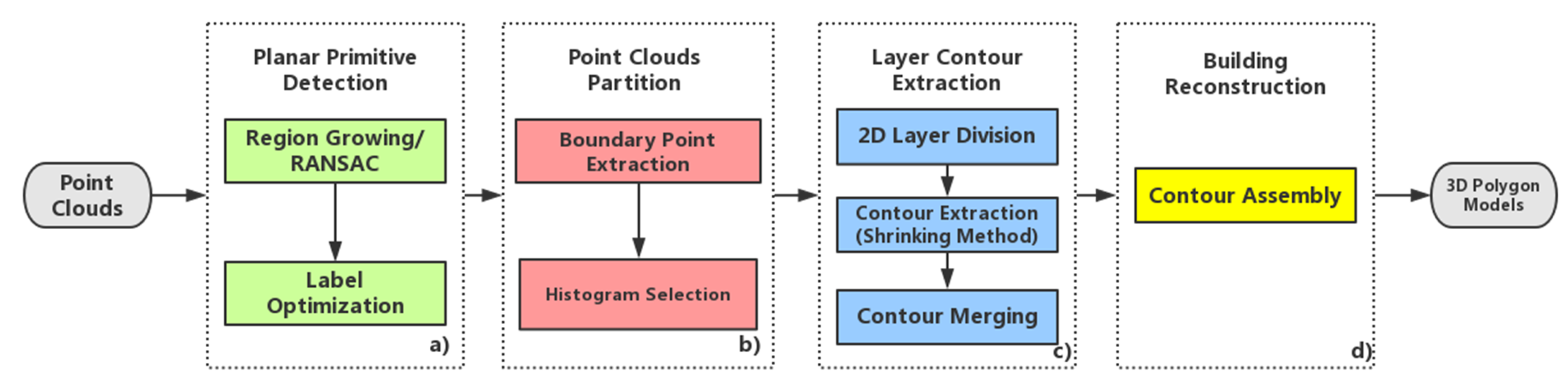
As shown in Figure 2, this approach contains four primary steps. To reconstruct the indoor space, we employ a multi-label method to detect the planar primitives through a global optimization based on the region-growing and random sample consensus (RANSAC) algorithms. Subsequently, the point clouds are sliced into several pieces along the vertical direction. Given the representative slices of the points, the contours of these slices can be extracted by a shrink-wrapping method. Finally, we assemble these 2D contours to constitute 3D building models.
3.2. Planar Primitive Detection
In this section, we detect the planar primitive to extract the planar features for further processing. The detection of planar primitives can be summarized as fitting the mathematical model to the data. The solutions to this problem can be classified into three types: A RANSAC-based algorithm, a region-growing-based algorithm, and a parameter space-based algorithm.
We first use the region-growing algorithm to gain the initial planar primitives. To refine these initial labels of planar primitives, a multi-label graph cuts optimization method is utilized. Through this label optimization step, most of the erroneously labeled primitives can be revised. Compared with other detection methods, this approach can segment the point clouds in a suitable scale.
3.2.1. Initial Planar Primitive Extraction
First, we perform the region-growing method to obtain the initial planar primitives from the filtered point clouds. The region-growing technique aims at finding a maximum set of points in the neighborhood. There are two key conditions of region-growing: (1) Propagation criterion denoting that the growing process is supposed to satisfy a criterion according to the features such as the normal, curvature, and point distributions, and (2) termination criterion, which is the ending condition of the propagation. This technique is widely used in point clouds segmentation by testing every neighboring point for the angle difference between the normals of the seed points and neighboring points.
In our case, we set up the growing criterion as the following equation:
where represents the normal of the current seed point, and denotes the points’ normals in the neighborhood. is the threshold to determine whether two points belong to the same plane (e.g., ). In practice, we use the Fast Library for Approximate Nearest Neighbors (FLANN) [20] to speed up the neighboring points search (e.g., 20 nearest points). Since the selection of seed points affects the quality and the speed of detection, we choose the points with minimal curvature in the unassigned point set.
Figure 3 shows the result of the region-growing. Although the region-growing method can obtain most of the correct planar primitives, some points belonging to the same wall are assigned to different labels. As shown in Figure 3, there are two situations of wrong segmentation: Overlapping and separating. The left section in Figure 3 illustrates points belonging to the same wall separated into several overlapping pieces. This is mainly caused from by scanning and registration errors. Another situation of the erroneous detection is that the single wall is divided into several non-overlapping parts. As shown in the right of Figure 3, the interested plane has been divided into three parts (i.e., blue, red, and green). This is because the indoor walls are not absolutely smooth, which gives rise to the normal inconsistency. Therefore, we merely utilize the result of region-growing as the initial assignment of point clouds and apply a refinement process to solve aforementioned problems.
3.2.2. Planar Primitive Optimization
Given the initial planar primitives, we apply an optimization method to solve the above-mentioned overlapping and separating problems. This process can be concluded as a label merging procedure which combines the erroneously segmented primitives to correct labels.
Starting from the initial segmentation, we can utilize the RANSAC plane fitting method to gain the initial parameters of planes. The merging process can be implemented in consideration of the planes’ normals and the mass centers of the planes. For instance, if a pair of planes satisfies the following conditions, we prefer to merge them to the identical plane: (1) The inconsistency of plane normals is smaller than a threshold (e.g., ), and (2) the distance between the mass centers of these two planes are smaller than a certain Euclidean distance (e.g., 0.5 m). If we consider these two conditions, we can improve the initial detection to some extent. Figure 4c indicates that these four planes (D, E, F, and G) are merged to the same plane. While the planes D, E, and F belong to the identical wall, plane G is not on the plane consisted by the other three primitives. Since these two planes are parallel and close to each other, it is difficult to find appropriate thresholds to guarantee that the wall segments on the identical wall can be merged while the nearby parallel walls can be separated. Figure 4b is another instance indicating that the parallel wall structures cannot be recognized.
Because the approach considering plane directions and mass centers cannot take nearby parallel walls into account, we apply a global optimization method to refine these two conditions. Through this optimization, the parallel planes tend to be separated while the co-planar planes are expected to be merged. Thus, we convert the merging problem to a labeling problem and solve it by minimizing the multi-label energy via graph cuts [21]. The combined energy function is as follows:
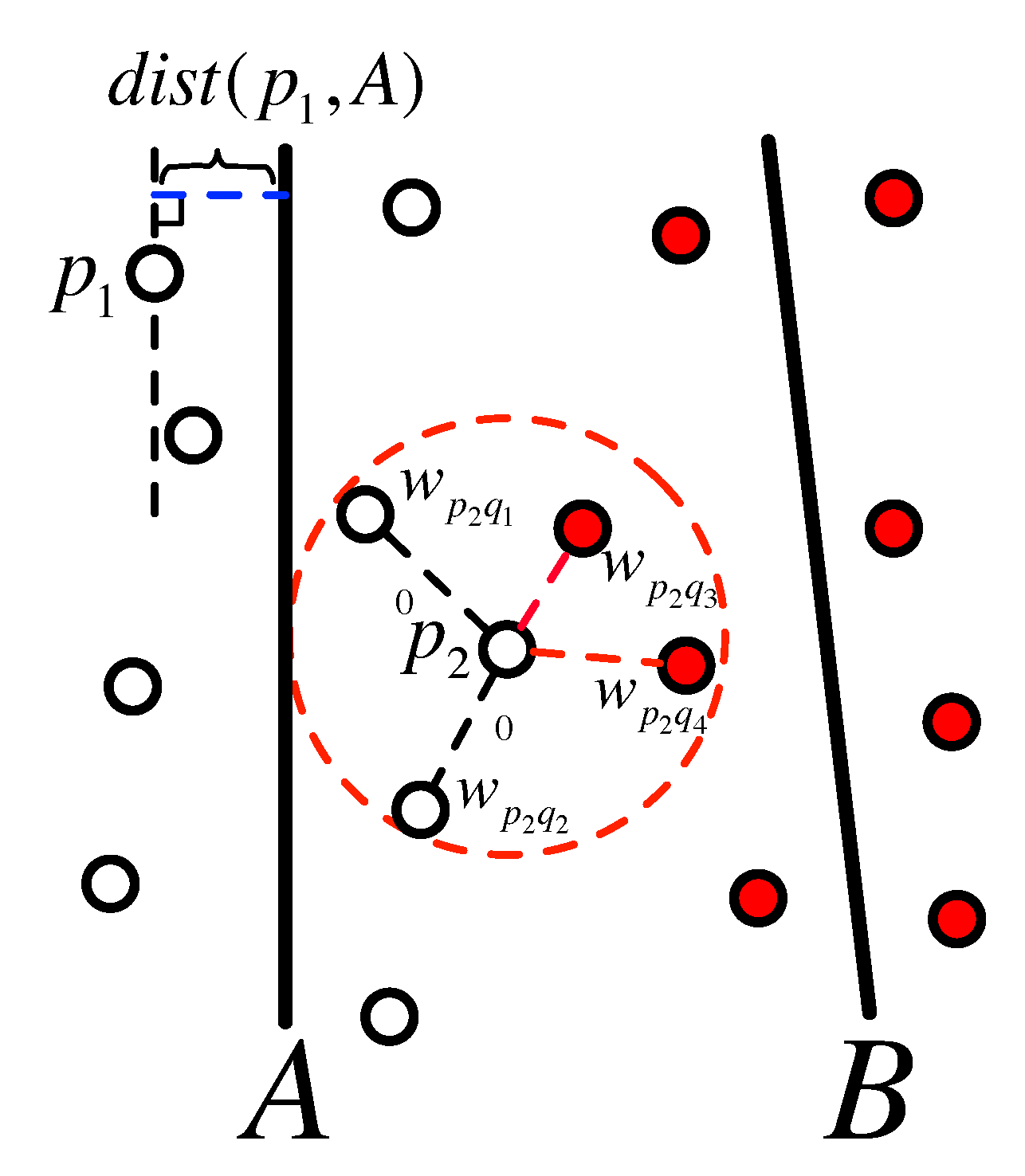
where the three terms are data term, smoothness term and label term, respectively. The first term is the data term representing the penalty of assigning a point to a particular label. The data term is calculated using Equation (3). As illustrated in Figure 5, is the perpendicular distance from a point to its fitting plane.
The second term is the smoothness term which is used to guarantee the smoothness in the neighborhood. We define the neighborhood of points as the k-nearest neighbors (e.g., ). The point in Figure 5 shows an instance where the points in the circle are its neighboring points. The points and are assigned to the same label as . In this case, the smoothness costs are equal to 0. The points and are assigned to the different labels, hence the smoothness cost can be calculated by the following equation:
where is the pairwise distance. We set m according to the common spacing of points. The is an indicator function for all the same label points in the k-nearest neighbor. Because our objective is to minimize the energy function, it tends to change the labels in the neighborhood if the cost of smoothness term can be decreased by adjusting the current label of point p to its neighboring label.
Since our goal is to merge the co-planar planes and retain the parallel planes, we utilized the third label term to penalize a large number of labels. We favored the fewer number of labels and encouraged the reduction of the redundant planes. Therefore, when the plane’s label cost was large, we prefered to merge this plane to the neighboring plane or discard this plane rather than retain it. The label term is defined as
where n is the number of labels and , , are the point number of current label, the maximum and minimum point number in all labels, respectively. Combining with , an indicator function in Equation (2), we can determine whether the label l will be retained or discarded.
To minimize the aforementioned energy function, we utilized the extended -expansion method developed by Delong et al. [21]. The algorithm converts the multi-label problem to a set of binary labeling problems and utilizes graph-cuts to minimize it. The minimization process is an iterative way to find the optimal labels for the data points until the energy function cannot be decreased [22]. After each iteration, if the value of energy function was decreased, we updated the current labels. The result of primitive detection method can be seen in Figure 6, where the co-planar primitives and parallel primitives are recognized correctly.
3.3. Point Cloud Partition
Given the planar primitives, a point cloud partition algorithm was employed to slice the vertical primitives into several layers. Since these layers always share repetitive structures on the upward direction, we utilized the histogram of boundary points to eliminate the redundant layers. Finally, we selected the representative layers to facilitate the contour extraction.
Figure 7a illustrates the vertical planar primitives extracted by normals. We sliced the point clouds to several consecutive blocks along the upward direction. Several 2D layers could be obtained through 2D projections as shown in Figure 7b. Subsequently, a least square linear fitting could be applied to extract linear primitives based on labels and orientations on each 2D layer. However, these 2D layers possessed considerable redundancy which decreasedd the efficiency of post-processing. For instance, the layers with elevations from 40 cm to 55 cm in Figure 8 shared almost the same structures which were supposed to be merged to one representative layer.
3.3.1. Boundary Point Extraction
In this section, we extract the feature points to facilitate the representative layers selection. We utilize the 3D boundary as feature points because of the following reasons: (1) The boundary of planar primitives retains most wall information (i.e., position, orientation, and height), (2) the boundary points can avoid the repetitive structures which share the same geometry on the vertical direction (e.g., as shown in Figure 8, the bottom three layers share the same geometry on the vertical direction). A convex hull-based method [23] has been employed to extract boundaries from detected planar primitives. To be specific, the points on planar primitives can be projected onto the RANSAC fitted planes and the convex hull (see Figure 9a) can be determined by these projected points. Subsequently, we determined the boundary points as when the distances from the projected points to the key points on convex polygons (see Figure 9b) are less than a given threshold (e.g., 0.05 m).
3.3.2. Representative Layer Selection
Although the vast majority of buildings share the same geometry, the number of boundary points varies in different layers. The changing number of boundary points reflects the changes of structures (see Figure 9c). Therefore, we constructed a histogram from the boundary points along the upward direction to select representative layers. In practice, starting from the floor to the ceiling level, we set a given bin size (e.g., 0.05 m) for the voting process and identified the local maximum from the histogram. Figure 10 shows the histogram of boundary points. The point clouds are partitioned into 67 blocks with the bin size of 0.05 m. Through identifying the peaks of histogram, we can extract nine layers to represent the whole building.
Given the peaking elevations of the histogram, a set of representative layers can be determined as depicted in Figure 11. The enlarged view of Figure 11a indicates that these selected layers could retain the structural changes along the vertical direction. As a consequence, the shapes of the bay windows could be kept. By means of representative layers selection, the large number of layers could be consolidated without dropping out structural information. Moreover, we converted the 3D reconstruction problem to several 2D layer reconstruction problem which was more feasible for further processing.
3.4. Layer Contour Extraction
After the representative layers were determined, we employed a “divide-and-merge” strategy to extract the contour of each layer. We first segmented the 2D layers into several parts for simplifying the shapes of contours. Subsequently, a shrink-wrapping-based approach was utilized to extract each piece of the contour. Finally, we integrated these parts into a complete contour. To this end, the wall elements could be retrieved from the contours of the representative layers.
3.4.1. 2D Layer Division
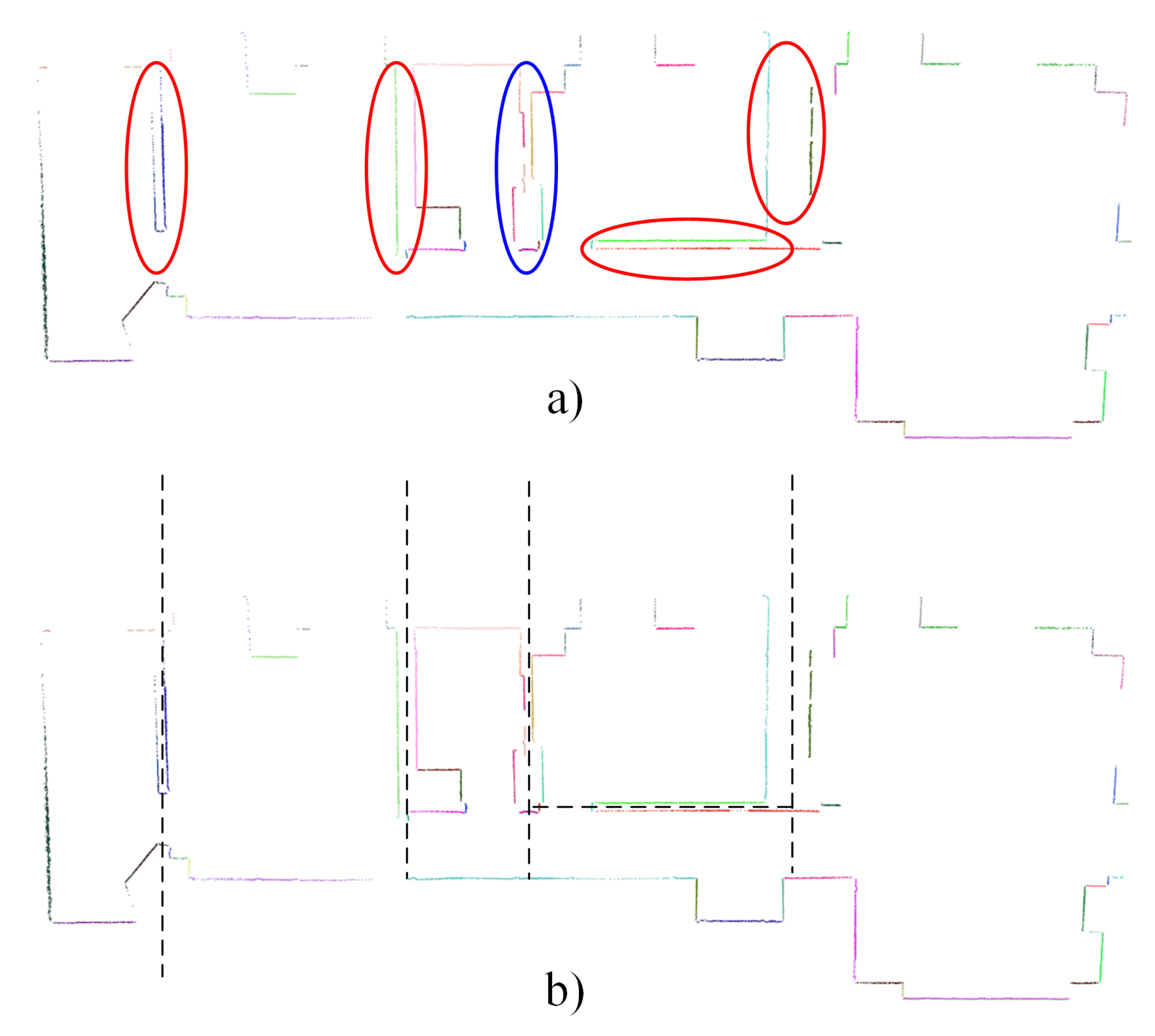
With the observation of indoor point clouds, there are two types of point distributions among wall elements: inner walls and outer walls [17]. Accordingly, we segmented the point clouds in these layers on the basis of inner wall point distribution. In practice, the first step is to determine the positions of inner walls, and then the segmentation can be completed by extending centre lines of inner wall structures. Actually, the localization of inner walls could be implemented by searching for parallel structures in a given distance. In our experiment, we set up the searching range as 0.5–0.9 m along the perpendicular direction of each linear primitive. Thus, the division line could be extracted from the bisector of two parallel linear primitives. However, sometimes the inner wall was labeled with different classes as indicated by the blue circle in Figure 12a. A mergence of adjacent division lines was required. By introducing division lines, we partitioned point clouds into several parts which could effectively convert a complicated floor plan to several simple sub-floorplans. As shown in Figure 12b, the representative layer extracted previously was divided into six parts. Note that some parts only contain one individual room while others involve parts of rooms or more than one room. As our reconstruction method was not based on the room, it did not affect the result of reconstruction. Our goal was only to obtain simple sub-floorplans here, not the room segmentation.
3.4.2. Contour Extraction
Inspired by the shrink-wrapping method from mesh reconstruction [24], we utilized a shrinkage process to obtain the regularized sub-contours. After that, we merged them along with the localizations of inner walls to complete the extraction of the contours. By this means, the boundary of each contour could represent the outer wall elements, and the inner wall elements could be recovered simultaneously.
The shrink-wrapping method is a classical geometry-processing algorithm which has been widely utilized in mesh reconstruction, simplification, and remeshing [25,26]. The basic principle behind shrink-wrapping is in its simulating process that a membrane is shrinking and finally wrapping onto an object. Therefore, the iso-surface of the reconstructed mesh is the wrapping membrane. Using point clouds as input, a convex hull is constructed as the initial approximation (“the membrane”). Consequently, the shrinkage is completed by incrementally deleting triangles until all points lie on the reconstructed surface (“wrapping on the object”). The advantages of shrinking-wrapping are the robustness and toleration of most point clouds. Despite these two advantages, our implementation could produce water-tight and regularized contours. The main differences between our case and the traditional shrink-wrapping approach are three-fold: (1) The 2D application scenario, (2) the object of shrinkage, and (3) the strategy of the shrinking process. The detailed descriptions of (2) and (3) are in the following.
- (1)
- Sub-Contour Extraction
The object of shrinkage: Compared with the conventional shrinking method, the object of our approach is linear primitive. Most of the wall elements are perpendicular to each other in the indoor environment, which means that there are two principle directions of each contour. As shown in Figure 13, the red lines denote the vertical primitives (type I), and the green lines indicate the horizontal primitives (type II). These two types of primitives are the dominant directions of the building. We can build a boundary box from the dominant directions as an initial approximation for the shrinkage. Although most of buildings are conforming to two dominant directions or the Manhattan-World assumption, there are not uncommon for the non-perpendicular wall elements in the real world. Accordingly, we introduce the arbitrary primitive as the type (type III) of linear primitive. Part 1 of Figure 13 shows an instance for the arbitrary primitive (depicted in blue color).
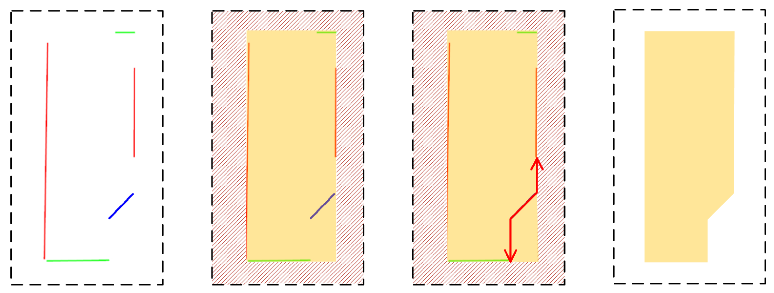
The strategy of Shrinkage: Taking the linear primitives of sub-contours as input, we classified these primitives into two sets as and . contained the type I and II primitives which were the dominant directions of the sub-contours. was the set of arbitrary primitives (type III) which would be considered in the later step of sub-contour extraction. We built a rectangular bounding box based on the two dominant directions as the initial approximation (see Figure 14). To initialize the elements in set B, we assigned the linear primitives in according to the directions and distances. The rectangles with dash lines in Figure 14 are the illustrations of the bounding box. Accordingly, we assigned the primitives to nearest edges of bounding box as shown in the right of Figure 14.
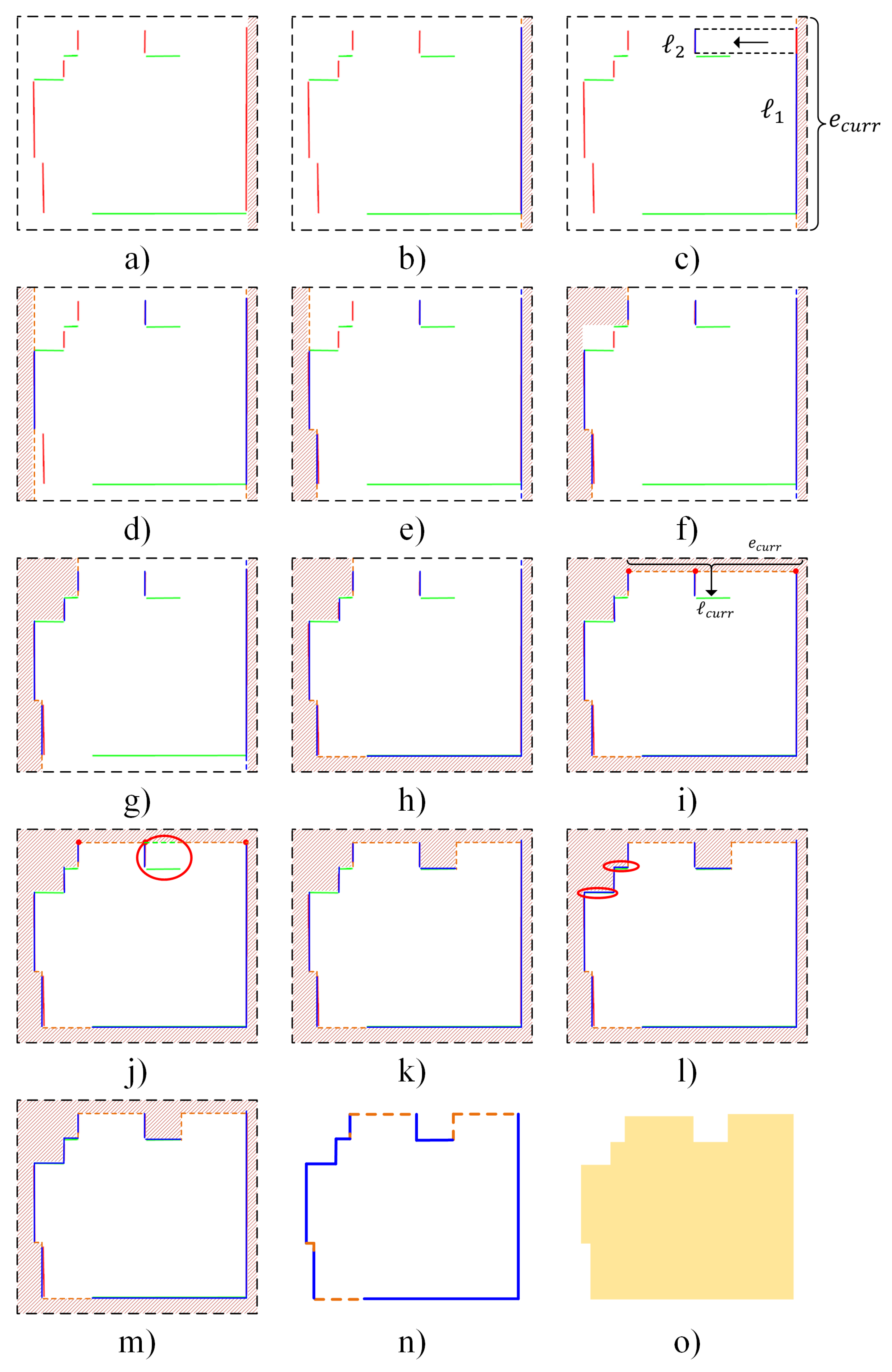
After initialization, the shrinkage was completed primitive-by-primitive. Selecting a primitive in the set , we extended the current boundary at first. Subsequently, shrinking was stopped when the extended boundary encountered other primitives (see Figure 15d–f). It is noted that the parts fitting to the real primitive would be considered as the determined contour (blue lines). Other parts will be the pending contour (orange dash lines) which might be changed subsequently. Despite the aforementioned situation, there are two extra situations to be checked:
(1) As depicted in Figure 15c, the projection of on current boundary was fully included, and possessed a longer distance to than . Therefore, considering the projecting inclusion, we shrunk the current edge (depicted in blue) to . To sum up, if the projection of farther primitive was fully included into the current extending edge, we shrunk the corresponding part to this farther primitive as a new determined edge.
(2) We needed to consider the situation where the shrinking edge would intersect with perpendicular primitives. As shown in Figure 15i, the operating edge would encounter perpendicular primitives at the red points before arriving the target primitive . To this end, we only adjusted the overlapping parts as shown in the red circle of Figure 15j. The remaining parts would only be shrunk to the intersected points (denoted as red points in Figure 15i). The adjusting result is depicted in Figure 15k.
When all primitives in assigned to set B were processed, we were supposed to obtain a contour consisting of determined edges and pending edges (see Figure 15n,o). According to the previous discussion, most of the sub-contours did not contain the arbitrary linear primitive meaning that the . However, in part 1 of Figure 13, the type III primitive did exist. Consequently, a post-processing step was required to deal with such a situation. In practice, in order to create new non-perpendicular edges in the current contour, we linked the endpoints of linear primitives in to their nearest endpoints in . After that, the redundant parts would be cut off from the current polygon to determine the final sub-contour. An instance of processing arbitrary primitive is depicted in Figure 16. It is noteworthy that the line with arrows represents the new boundary edge added to the current boundary. Figure 17 shows the results of sub-contours extraction according to the previously discussed shrinking strategy.
- (2)
- Sub-Contour Mergence
Once we obtain the sub-contours, it is easy to merge them to generate a large contour as the initial contour (see Figure 18a). In general, the sub-contour mergence can be completed through the following steps: (1) Initial mergence, (2) virtual walls’ elimination, and (3) connection recovery.
The sub-contour extraction generates a closed boundary even there are no underlying linear primitives. Thus, in the joint connections between sub-contours may exist virtual inner walls. Therefore, we eliminate the boundaries on the joint connections between sub-contours (see the red lines depicted in Figure 18b).
Despite the redundant boundary between the adjacency of sub-contours, there may exist some isolated sub-contours (e.g., part 1 in Figure 17). However, the acquisition of point clouds is completed in the indoor scenes which means all the rooms are connecting to each other. Thus, we need to recover the connection information which has been ignored in the previous steps. To this end, we search the overlapping linear primitive along the boundary of isolated primitives. As shown in Figure 18b, the linear primitives underlying the boundary between the sub-contours 1 and 2 are overlapping to each other. Moreover, these two edges of boundaries share the same vacancy which denotes the location of the missing connection. The blue edges indicate the area of vacancies, and the green rectangles are the recovered connections. An illustration of the extracted contour is shown in Figure 18c, and the overall process of contour extraction is summarized in Algorithm 1.
| Algorithm 1: Contour Extraction. |
 |
3.5. Building Reconstruction
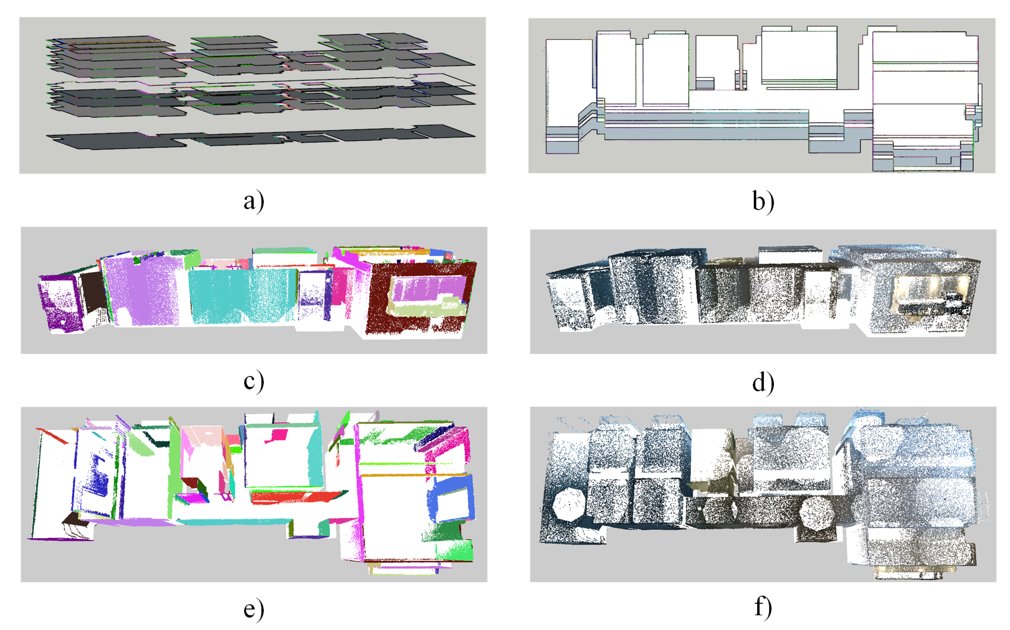
With the extracted contours of representative layers (see Figure 19a), we assembled these contours to generate 3D building models. However, directly extruding contours to create the building model causes a jagged, unaligned mesh as shown in Figure 19. Instead, we registered each contour layer-by-layer from bottom to top through averaging the location of edges with the predefined distance (e.g., 0.05 m) and angle (e.g., ). Figure 19 contains the final reconstructed models overlapping with the original point clouds (Figure 19d,f) and labeled vertical point clouds (Figure 19c,e). For the sake of clarity, we truncated the ceiling to show the performance of the interior reconstruction in Figure 19c,e.
4. Experiments
In this section, we present the experimental results of the proposed methods. The performance and effectiveness of the proposed method are evaluated through various datasets. In addition, a quantitative experiment compared with other’s algorithms is conducted to evaluate the accuracy and performance of our method. Finally, we analyze the influence of parameters to the output models.
4.1. Datasets
The datasets utilized in the experiments are from both mobile and terrestrial datasets in indoor environments (e.g., offices and departments). The terrestrial scanning point clouds is provided by Ikehata et al. involving channels such as 3D coordinates, color information, reflecting intensity, and normals [8]. The mobile scanning point clouds were acquired by a trolley-based IMMS with 3D coordinates and intensity information [17] for validating the the extensibility of our methods. The datasets used in the experiments are listed in Table 1.
4.2. Modeling Outputs
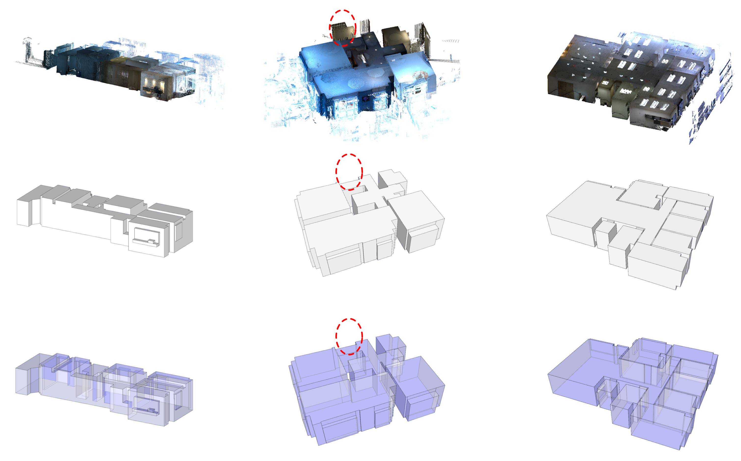
Firstly, we utilized three terrestrial point clouds to test the proposed reconstruction method from 3D primitives. Table 2 lists the statistics of the reconstructed outputs and the parameters need to be adjusted in the reconstruction. Figure 20 contains the original point clouds and the reconstructed results. We also provided the reconstructed models rendered with a transparent view to display the inner spaces. In general, the proposed method can offer detailed 3D models including non-Manhattan structures, different heights of ceilings, and prominent structures.
In the first and third datasets, all rooms have been reconstructed successfully. Nevertheless, one room in Apartment 2 was discarded in the reconstruction. The red circles in the middle column of Figure 20 denote the corresponding locations in the original point clouds and reconstructed models. The main reason behind this phenomenon is that this room was scanned incompletely. Furthermore, the noise filter aggravated the reduction of points, especially in the lower density area. Therefore, when the algorithm detected planar primitives, the number of supporting points in this room was insufficient.
4.3. Parameters
In this section, we clarify the reason for parameter settings by tuning different parameters. Some explanations and analyses will be given to explore the suggested values of our methods. We classify the parameters according to the different modules into planar primitive detection, contour extraction, and building reconstruction (please refer to Table 3).
Parameters of planar primitive detection: There are three parameters to be predefined in this category. is the threshold for the normal inconsistency between the current seed and neighboring points during the region-growing. k is the radius of neighborhood, which is used in region-growing and smoothness term calculation. is a parameter to adjust the weight of smoothness term denoting the average space of the point clouds. We can calculate it through stuying the density of point clouds.
Parameters of contour extraction: The parameters utilized in the contour extraction are primarily based on the distance. The values of these parameters are insensitive since the indoor structures of civil architecture are similar. Therefore, the parameters do not need to be tuned for different point clouds.
and are two parameters leveraged in point cloud partition. is the parameter to restrict the distance from point clouds to key points of convex hulls. A large value of considers more points as boundary points which decrease the discrepancy of the histogram. We suggest that the value of is less than or equal to the bin size (1/2–1 times of ). denotes the bin size of the histogram in the representative layer selection as well as the interval of slice along the vertical direction. Although approaching layers keep more indoor structures as shown in Figure 21a, the supporting points of each layer suffer from a corresponding decrease. This decrease causes the problem in linear primitive extraction due to insufficient supporting points. On the other hand, in spite of the greater interval that can consolidate the 2D projection layer (see m in Figure 21d) and accelerate the processing speed, lots of structure information is thrown away simultaneously. Considering the trade-off between the processing speed, layer consolidation, and indoor structures, we set the interval threshold as 0.05–0.1 m.
denotes the searching radius of parallel inner walls to divide the 2D point clouds into several subsets for simplifying the contour regularization. Although increasing the searching radius can improve the ability of locating parallel structures, a large value of gives rise to the over-partition. As illustrated in Figure 22, the smaller value dismisses some large interval parallel walls. However, a large searching distance introduces errors as indicated in blue circle of Figure 22b. Typically, the thickness of inner walls is about 20 cm. Therefore, in order to improve the tolerant rate and deal with the exceptional case as in Figure 22, we set a reasonable range of as 0.5–1.0 m.
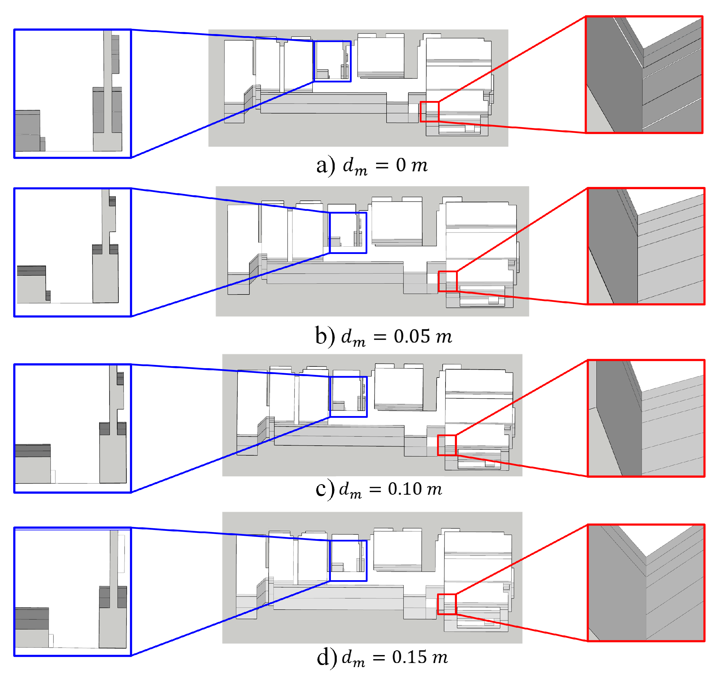
Parameters of building reconstruction: Our strategy of building reconstruction was to generate 3D building models by assembling the contours of different representative layers. and control the level-of-detail in the final models. In practice, we mainly adjusted the model’s level-of-detail by due to the observation that the inconsistency of distances regarding linear primitives was more significant than the inconsistency of angles. A large value of discards the details of models as indicated by the blue rectangles in Figure 23c,d. However, if we assembled the contour without mergence, the output model would be jagging and zig-zagging between layers. Figure 23a is the initial model without mergence, and the boundaries of the model are jagging. In general, the inconsistency of boundaries was less than 0.2 m.
4.4. Quantitative Evaluation
To quantitatively evaluate the quality of modeling results, we used both realistic data and synthetic data. We took the distance from the point to its nearest reconstructing surface as the measurement metric. The reconstruction error could be seen in Figure 24. According to our test, the proposed method was to obtain averaging fitting errors at 3.35 cm.
We also manually created the building models and sampled them to generate synthetic data to evaluate the performance of the proposed method against different levels of noises (See Figure 25). As shown in Table 4, we appended Gaussian noises at = 5 mm, 10 mm, and 20 mm. The average fitting errors from the results to the ground truth were 0.407–3.213 cm.
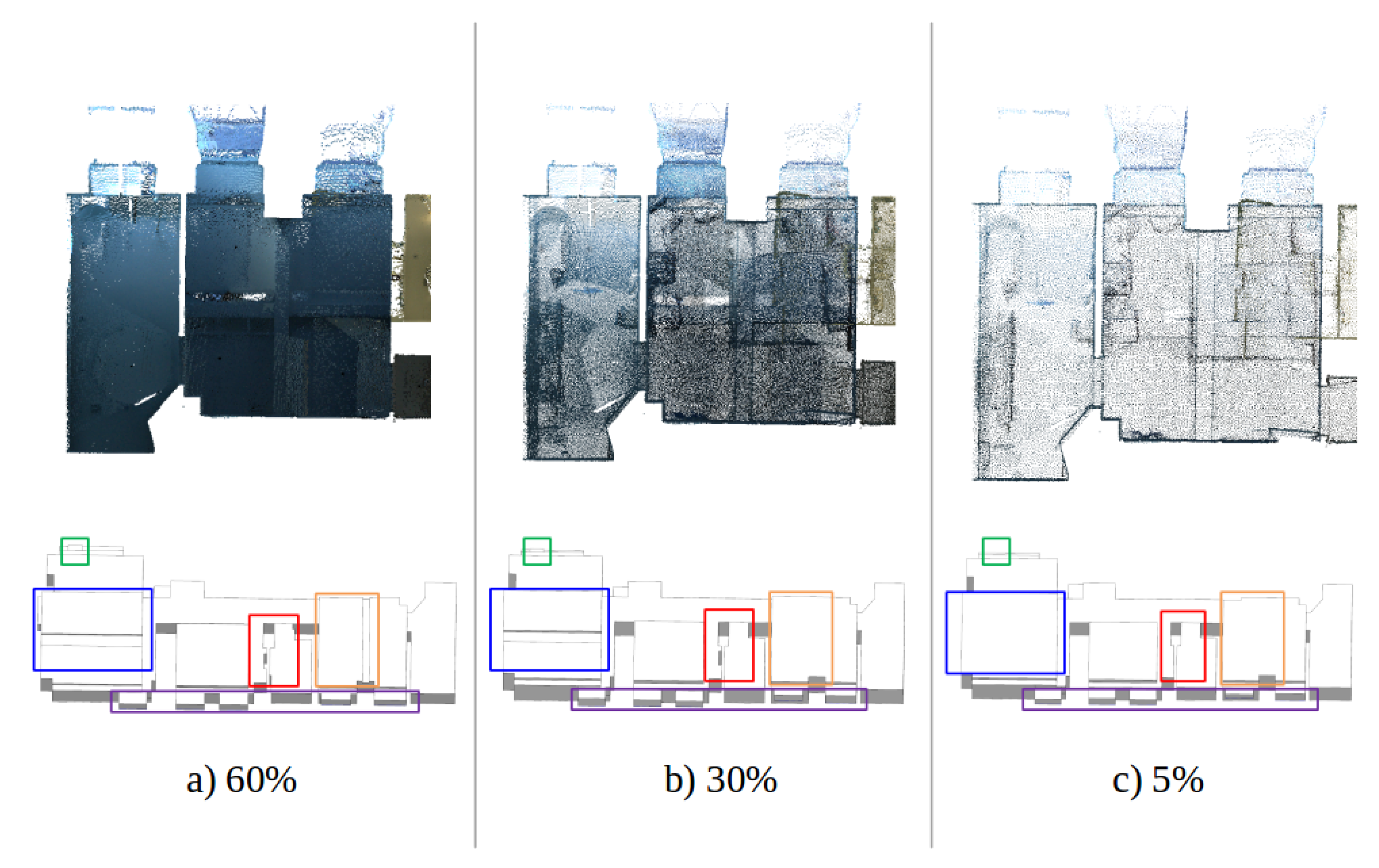
To evaluate the robustness towards sparse data, we sampled the original data to , , and (corresponding to Figure 26a–c). The results showed that our method could retain the major part of building even in point clouds. However, with the decreasing of point density, some details were discarded (e.g., uneven ceiling depicted in blue rectangle in Figure 26). The errors and detail deficiency were attributed to the sparse supporting points because of the insufficient extraction of representative layers.
4.5. Comparisons
In order to evaluate the performance, we conducted comparisons with two state-of-the-art methods, namely structured indoor modeling [8] and Manhattan-World urban reconstruction [10] (see Figure 27). Compared with the structured indoor modeling method, the proposed method generated more elaborate models, especially when recovering the complicated structures on the ceilings, and overhang building components (e.g., bay windows, windowsills). The method of structured indoor modeling required line-of-sight information to compute a score of free space to distinguish the indoor-outdoor spaces, which limited the capability of extension. Nevertheless, the proposed method from 3D primitives required nothing except the point clouds, which meant it could be applied to various types of point clouds.
With respect to another method named Manhattan-World urban reconstruction, our method had two advantages. As shown in Figure 27c,d, the reconstruction results of these two methods are comparable. However, our method could produce more compact models with fewer polygons. This is mainly because Li et al.’s method relied on the process of axis-aligned box selection, thus, the final model consisted of a stack of closed cuboids, which introduced redundant polygons. The second advantage of the proposed method was the capability of expressing the interior spaces of the building. Li et al.’s solution could recover the exterior of the building delicately, but the inner space was blocked by enclosed boxes (see the transparent view of Figure 27c). In contrast to their implementation, our method could represent the interior spaces with connections between different rooms. It is worth noting that the other two methods were based on the Manhattan-World assumption, which cannot reconstruct the non-perpendicular structures such as the slant walls indicated in the red rectangles of Figure 27.
Because the aforementioned two methods are designed merely for the terrestrial point clouds or cannot represent the inner space, we conducted another comparison with method proposed by Wang et al. [17]. We used the mobile laser scanning (MLS) point clouds to evaluate the extension capability of the 3D primitive reconstruction method. In practice, the large number of point clouds lead to a crash in 3D primitive methods because of the deficiency of memory. The bottle-neck of processing large-scale point clouds for planar primitive detection was the insufficient memory due to huge computational costs. According to our experiment, it took 30 min for 10 million points on a desktop computer (Intel i7-4770, 10 GB Ram). Therefore, we downsampled this dataset to approximate 10 million points for the experiment.
In contrast to the previous method, the proposed method possesses the advantages that it can generates more detailed models in the following aspects: (1) It can represent the actual thickness of walls, and (2) the planar primitives improved the capability of recovering small corners of buildings. Although our method provides more detail models, it gets stuck when encountering incomplete or low density point clouds (also shown in Figure 20). As illustrated in Figure 28, the proposed method fails in recovering some ceilings because the density of points decreases with the increasing level of architectures.
5. Conclusions
This paper proposes a layer-wise method for indoor as-built spaces modeling using 3D planar primitives. The layer-wise strategy slices the point clouds into several pieces on the vertical directions which retains the structural changing in the walls and ceilings. By using 3D planar primitives, detailed structures such as the thickness of inner walls and protruding structures can be retrieved. Compared with the existing methods, our methods can automatically generate models with a higher level of details, and enhance the geometric representation of models. To our knowledge, few existing methods for indoor building modeling can deal with both mobile and terrestrial point clouds. The proposed reconstruction method provides a possible solution, which does not have the particular requirement for input point clouds, and does not rely on any extra information such as the line-of-sight record or the scanner trajectory. The assessment demonstrates the effectiveness and accuracy of our method, and the capability against sparse and noisy data.
In order to enhance the details of models, in future work, we will focus on exploring more geometric primitives (e.g., sphere and cylinder) to deal with non-planar structures. We also intend to integrate the multi-story building detection (i.e., stairs) for modeling a multi-story building in one pipeline.
Author Contributions
Conceptualization, L.X.; methodology, L.X.; software, L.X.; writing—original draft preparation, L.X.; writing—review and editing, L.X., Z.M., D.C., R.W.; visualization, L.X., Z.M.; supervision, R.W.
Funding
This work was supported by the Natural Sciences and Engineering Research Council of Canada (NSERC).
Conflicts of Interest
The authors declare no conflict of interest.
References
- Tang, P.; Huber, D.; Akinci, B.; Lipman, R.; Lytle, A. Automatic reconstruction of as-built building information models from laser-scanned point clouds: A review of related techniques. Autom. Constr. 2010, 19, 829–843. [Google Scholar] [CrossRef]
- Jung, J.; Hong, S.; Jeong, S.; Kim, S.; Cho, H.; Hong, S.; Heo, J. Productive modeling for development of as-built BIM of existing indoor structures. Autom. Constr. 2014, 42, 68–77. [Google Scholar] [CrossRef]
- Previtali, M.; Díaz-Vilariño, L.; Scaioni, M. Indoor building reconstruction from occluded point clouds using graph-cut and ray-tracing. Appl. Sci. 2018, 8, 1529. [Google Scholar] [CrossRef]
- Khoshelham, K.; Elberink, S.O. Accuracy and resolution of kinect depth data for indoor mapping applications. Sensors 2012, 12, 1437–1454. [Google Scholar] [CrossRef] [PubMed]
- Lehtola, V.V.; Kaartinen, H.; Nüchter, A.; Kaijaluoto, R.; Kukko, A.; Litkey, P.; Honkavaara, E.; Rosnell, T.; Vaaja, M.T.; Virtanen, J.P.; et al. Comparison of the selected state-of-the-art 3D indoor scanning and point cloud generation methods. Remote Sens. 2017, 9, 796. [Google Scholar] [CrossRef]
- Bosse, M.; Zlot, R.; Flick, P. Zebedee: Design of a spring-mounted 3-d range sensor with application to mobile mapping. IEEE Trans. Robot. 2012, 28, 1104–1119. [Google Scholar] [CrossRef]
- Budroni, A.; Böhm, J. Automatic 3D modelling of indoor Manhattan-World scenes from laser data. Proc. Int. Arch. Photogramm. Remote Sens. Spat. Inf. Sci. 2010, 115–120. [Google Scholar]
- Ikehata, S.; Yang, H.; Furukawa, Y. Structured indoor modeling. In Proceedings of the IEEE International Conference on Computer Vision, Santiago, Chile, 7–13 December 2015; pp. 1323–1331. [Google Scholar]
- Mura, C.; Mattausch, O.; Villanueva, A.J.; Gobbetti, E.; Pajarola, R. Automatic room detection and reconstruction in cluttered indoor environments with complex room layouts. Comput. Gr. 2014, 44, 20–32. [Google Scholar] [CrossRef] [Green Version]
- Li, M.; Wonka, P.; Nan, L. Manhattan-World urban reconstruction from point clouds. In European Conference on Computer Vision; Springer: Cham, Switzerland, 2016; pp. 54–69. [Google Scholar]
- Previtali, M.; Barazzetti, L.; Brumana, R.; Scaioni, M. Towards automatic indoor reconstruction of cluttered building rooms from point clouds. ISPRS Ann. Photogramm. Remote Sens. Spat. Inf. Sci. 2014, 2, 281–288. [Google Scholar] [CrossRef]
- Oesau, S.; Lafarge, F.; Alliez, P. Indoor scene reconstruction using feature sensitive primitive extraction and graph-cut. ISPRS J. Photogramm. Remote Sens. 2014, 90, 68–82. [Google Scholar] [CrossRef] [Green Version]
- Sanchez, V.; Zakhor, A. Planar 3D modeling of building interiors from point cloud data. In Proceedings of the 2012 19th IEEE International Conference on. IEEE Image Processing (ICIP), Orlando, FL, USA, 30 September–3 October 2012; pp. 1777–1780. [Google Scholar]
- Nakagawa, M.; Yamamoto, T.; Tanaka, S.; Shiozaki, M.; Ohhashi, T. Topological 3d Modeling Using Indoor Mobile LIDAR Data. Int. Arch. Photogramm. Remote Sens. Spat. Inf. Sci. 2015, 40, 13–18. [Google Scholar] [CrossRef]
- Wang, Q.; Yan, L.; Zhang, L.; Ai, H.; Lin, X. A Semantic Modelling Framework-Based Method for Building Reconstruction from Point Clouds. Remote Sens. 2016, 8, 737. [Google Scholar] [CrossRef]
- Xiao, J.; Furukawa, Y. Reconstructing the world’s museums. Int. J. Comput. Vis. 2014, 110, 243–258. [Google Scholar] [CrossRef]
- Wang, R.; Xie, L.; Chen, D. Modeling indoor spaces using decomposition and reconstruction of structural elements. Photogramm. Eng. Remote Sens. 2017, 83, 827–841. [Google Scholar] [CrossRef]
- Turner, E.; Zakhor, A. Floor plan generation and room labeling of indoor environments from laser range data. In Proceedings of the 2014 International Conference on IEEE Computer Graphics Theory and Applications (GRAPP), Lisbon, Portugal, 5–8 January 2014; pp. 1–12. [Google Scholar]
- Turner, E.; Cheng, P.; Zakhor, A. Fast, automated, scalable generation of textured 3d models of indoor environments. IEEE J. Sel. Top. Signal Process. 2015, 9, 409–421. [Google Scholar] [CrossRef]
- Muja, M.; Lowe, D.G. Fast approximate nearest neighbors with automatic algorithm configuration. VISAPP (1) 2009, 2, 2. [Google Scholar]
- Delong, A.; Osokin, A.; Isack, H.N.; Boykov, Y. Fast approximate energy minimization with label costs. Int. J. Comput. Vis. 2012, 96, 1–27. [Google Scholar] [CrossRef]
- Isack, H.; Boykov, Y. Energy-based geometric multi-model fitting. Int. J. Comput. Vis. 2012, 97, 123–147. [Google Scholar] [CrossRef]
- Yi, C.; Zhang, Y.; Wu, Q.; Xu, Y.; Remil, O.; Wei, M.; Wang, J. Urban building reconstruction from raw LiDAR point data. Comput.-Aided Des. 2017, 93, 1–14. [Google Scholar] [CrossRef]
- Jeong, W.K.; Kim, C.H. Direct reconstruction of displaced subdivision surface from unorganized points. In Proceedings of the 2001 Ninth Pacific Conference on IEEE Computer Graphics and Applications, Tokyo, Japan, 16–18 October 2001; pp. 160–168. [Google Scholar]
- Kobbelt, L.P.; Vorsatz, J.; Labsik, U. A shrink wrapping approach to remeshing polygonal surfaces. Comput. Graph. Forum 1999, 18, 119–130. [Google Scholar] [CrossRef]
- Van Overveld, K.; Wyvill, B. Shrinkwrap: An efficient adaptive algorithm for triangulating an iso-surface. Vis. Comput. 2004, 20, 362–379. [Google Scholar] [CrossRef]
Figure 1.
Multiple views of point clouds: (a) Top-down view of filtered point clouds. (b) Side-view of filtered point clouds. (c) The 2D projection of point clouds (the rectangles with different colors denote the corresponding structures in multi-view figures).
Figure 1.
Multiple views of point clouds: (a) Top-down view of filtered point clouds. (b) Side-view of filtered point clouds. (c) The 2D projection of point clouds (the rectangles with different colors denote the corresponding structures in multi-view figures).

Figure 2.
The flowchart of the proposed approach involving four major steps. (a) Planar primitive detection; (b) point clouds partition using boundary points; (c) layer contour extraction in the 2D space; (d) building assembly.
Figure 2.
The flowchart of the proposed approach involving four major steps. (a) Planar primitive detection; (b) point clouds partition using boundary points; (c) layer contour extraction in the 2D space; (d) building assembly.

Figure 3.
The result of region-growing: enlarged drawings show that the co-planar walls have been separated into several parts.
Figure 3.
The result of region-growing: enlarged drawings show that the co-planar walls have been separated into several parts.

Figure 4.
The results of plane refinement: (a) The point clouds before refinement, (b) plane A and plane B have been merged to plane C, and (c) planes D, E, F, and G have been combined into plane H. They are actually parallel planes (not belonging to the same plane).
Figure 4.
The results of plane refinement: (a) The point clouds before refinement, (b) plane A and plane B have been merged to plane C, and (c) planes D, E, F, and G have been combined into plane H. They are actually parallel planes (not belonging to the same plane).

Figure 5.
An illustration of labeling points and their fitting planes. The white dots and red dots represent the points with different labels assigned to plane A and plane B, respectively. The distances between points and planes are perpendicular distances. The points in the red circle illustrate the neighboring points of and the smoothness cost to the different points.

Figure 6.
The top-down view and side view results of planar primitive detection (rendered in different colors).
Figure 6.
The top-down view and side view results of planar primitive detection (rendered in different colors).

Figure 7.
Point cloud partition and linear fitting: (a) The planar primitives from vertical structures, (b) the 2D projections of consecutive blocks (each color represents ten layers), (c) the result of the linear fitting (Red lines: Vertical primitives; Green lines: Horizontal primitives).
Figure 7.
Point cloud partition and linear fitting: (a) The planar primitives from vertical structures, (b) the 2D projections of consecutive blocks (each color represents ten layers), (c) the result of the linear fitting (Red lines: Vertical primitives; Green lines: Horizontal primitives).

Figure 8.
The instance of repetitive layers sharing the same geometry on the vertical direction (truncated elevation from 40 cm to 55 cm).
Figure 8.
The instance of repetitive layers sharing the same geometry on the vertical direction (truncated elevation from 40 cm to 55 cm).

Figure 9.
The process of boundary points extraction: (a) Convex hull, (b) key points on the convex polygon, (c) boundary points.
Figure 9.
The process of boundary points extraction: (a) Convex hull, (b) key points on the convex polygon, (c) boundary points.

Figure 10.
The histogram of boundary points along the upward direction: The selected local maximum layers are bounded by the red rectangles (Figure 7b shows the total 67 layers).
Figure 10.
The histogram of boundary points along the upward direction: The selected local maximum layers are bounded by the red rectangles (Figure 7b shows the total 67 layers).

Figure 11.
The multi-view of representative layers (top-down view and side-view): (a) Enlarged bay window structure, and (b) selected layers retain different building structures.
Figure 11.
The multi-view of representative layers (top-down view and side-view): (a) Enlarged bay window structure, and (b) selected layers retain different building structures.

Figure 12.
The division process of 2D layer: (a) The localization of inner walls (blue circle: wall in multiple labels; red circle: Wall in the individual label), and (b) the layer division according to the inner wall positions.
Figure 12.
The division process of 2D layer: (a) The localization of inner walls (blue circle: wall in multiple labels; red circle: Wall in the individual label), and (b) the layer division according to the inner wall positions.

Figure 13.
The types of linear primitives in sub-contours: vertical primitives (red), horizontal primitives (green), and arbitrary primitives (blue). 1–6 indicate the sub-floorplans in the 2D layer.
Figure 13.
The types of linear primitives in sub-contours: vertical primitives (red), horizontal primitives (green), and arbitrary primitives (blue). 1–6 indicate the sub-floorplans in the 2D layer.

Figure 14.
Initialization of the bounding box: Assigning linear primitives to the edges of bounding box (the arrows indicate the assigning directions): (a) illustrations of the bounding box, (b) the primitives assigned to the nearest edges of bounding box.
Figure 14.
Initialization of the bounding box: Assigning linear primitives to the edges of bounding box (the arrows indicate the assigning directions): (a) illustrations of the bounding box, (b) the primitives assigned to the nearest edges of bounding box.

Figure 15.
The process of sub-contour shrinkage: (1) (a,b) and (d–h): ordinary shrinkage situations; (2) (c): extra situation one; (3) (i–l): extra situation two (see the shrinkage strategy); (4) (m,n): the extracted boundary of sub-contour: orange dashed lines: the pending edges; blue lines: the determined edges; (5) (o): the extracted sub-contour polygon model.

Figure 16.
Arbitrary primitive processing: Linkage and cutting (the blue line indicates the set of type III primitive—).
Figure 16.
Arbitrary primitive processing: Linkage and cutting (the blue line indicates the set of type III primitive—).

Figure 17.
The results of sub-contours extraction: The extracted contours are rendered in the yellow background (from layer 48). 1–6 indicate the sub-floorplans in the 2D layer.
Figure 17.
The results of sub-contours extraction: The extracted contours are rendered in the yellow background (from layer 48). 1–6 indicate the sub-floorplans in the 2D layer.

Figure 18.
The process of sub-contour mergence: (a) Initial mergence of sub-contours (1–6 indicate the extracted sub-contours), (b) merging refinement (enlarged to show the connections between sub-contours), (c) the result of contour extraction (red lines: Virtual connection walls; blue lines: Wall vacancies; green rectangles: The extracted connections).

Figure 19.
The process and results of building reconstruction: (a) The result of contour extraction (in layers), (b) the result of initial contour assembly, (c,d) the front view of building reconstruction overlapping with point clouds, and (e,f) the top view of reconstruction results. The colored point clouds in (c,e) represent the labels of segmentation, and the original point clouds are depicted in (d,f).

Figure 20.
Modeling outputs of the proposed method. From top to bottom: The original point clouds, the reconstructed models with ceilings, and the transparent view of models. The red circles denote the missing room in the reconstruction.
Figure 20.
Modeling outputs of the proposed method. From top to bottom: The original point clouds, the reconstructed models with ceilings, and the transparent view of models. The red circles denote the missing room in the reconstruction.

Figure 21.
The experimental results for different values of search radius : (a) Over-segmentation; (b,c) well-segmented; (d) under-segmentation.
Figure 21.
The experimental results for different values of search radius : (a) Over-segmentation; (b,c) well-segmented; (d) under-segmentation.

Figure 22.
The experimental results for different values of search radius : (a) Under-partition, and (b) over-partition. Red circle: Detected parallel structures; Blue circle: Over-partition situation; Dashed line: Partition boundaries.
Figure 22.
The experimental results for different values of search radius : (a) Under-partition, and (b) over-partition. Red circle: Detected parallel structures; Blue circle: Over-partition situation; Dashed line: Partition boundaries.

Figure 23.
The effects of the merging parameter to the final model: From 0 cm to 15 cm. (a) zig-zagging model without mergence; (b) proper merging parameter keeps the details of building; (c,d) details discard because of the over-mergence.
Figure 23.
The effects of the merging parameter to the final model: From 0 cm to 15 cm. (a) zig-zagging model without mergence; (b) proper merging parameter keeps the details of building; (c,d) details discard because of the over-mergence.

Figure 24.
Point clouds colored with distance between points and the reconstructed model.

Figure 25.
Accuracy evaluation on the synthetic data. First row: Point clouds with 5 mm, 10 mm, 20 mm Gaussian noise. Second row: Errors from the proposed method.
Figure 25.
Accuracy evaluation on the synthetic data. First row: Point clouds with 5 mm, 10 mm, 20 mm Gaussian noise. Second row: Errors from the proposed method.

Figure 26.
Sparse point clouds (with different downsampling rates) and corresponding output models: (a) sampling rate 60%; (b) sampling rate 30%; (c) sampling rate 5%.
Figure 26.
Sparse point clouds (with different downsampling rates) and corresponding output models: (a) sampling rate 60%; (b) sampling rate 30%; (c) sampling rate 5%.

Figure 27.
Comparisons with different methods: (a) the original point clouds; (b) the results from structured indoor modeling method (Ikehata et al. [8]); (c) the results from Manhattan-World urban reconstruction method (Li et al. [10]); (d) the results from the proposed method. From left to right: Side view, front view, and transparent view.

Figure 28.
The comparison of different methods on mobile scanning data. (a) Reconstruction from our method, (b) reconstruction from decomposition and reconstruction of structural elements [17], and (c) enlarged detail of outputs.
Figure 28.
The comparison of different methods on mobile scanning data. (a) Reconstruction from our method, (b) reconstruction from decomposition and reconstruction of structural elements [17], and (c) enlarged detail of outputs.


Table 1.
The description and statistics of the input datasets.
| Point Clouds | Apartment 1 | Apartment 2 | Office 1 | Office 2 |
|---|---|---|---|---|
| # of points [million] | 5.0 | 4.5 | 10.1 | 52.2 |
| # of stations | 15 | 14 | 32 | n/a |
| # of rooms | 6 | 5 | 10 | 18 |
Table 2.
Statistics of the output models.
| Output (from 3D Primitive) | Apartment 1 | Apartment 2 | Office 1 |
| # of rooms | 6 | 4 | 10 |
| # of vertices | 358 | 194 | 260 |
| # of faces | 689 | 390 | 522 |
| Parameters | Apartment 1 | Apartment 2 | Office 1 |
| 0.9 | 0.5 | 0.5 |
Table 3.
Parameters of proposed layer-wise method.
| Parameters | Values | Descriptions |
|---|---|---|
| Planar primitive detection parameters | ||
| The threshold for the region-growing. | ||
| k | 20 | The searching radius of neighborhood. |
| 0.01 | The threshold to adjust the weight . | |
| Contour extraction parameters | ||
| 1/2*–1* | The maximum distance to extract the boundary point in convex hull. | |
| 0.05 m | The bin size of histogram (equals to the distance between the vertical slice). | |
| * | The searching radius of the parallel inner walls. | |
| Building reconstruction parameters | ||
| 0.05 m | The merging distance for different contours. | |
| The merging angle for different contours. | ||
The symbol ‘*’ represents the parameters determined by the datasets.
Table 4.
Evaluation of synthetic data with different Gaussian noise.
| Synthetic Data | Maximum Error (cm) | Minimum Error (cm) | Average Error (cm) |
|---|---|---|---|
| Data 1 (5 mm) | 0.620 | 0.105 | 0.407 |
| Data 2 (10 mm) | 2.412 | 0.219 | 1.576 |
| Data 3 (20 mm) | 4.171 | 0.629 | 3.213 |
© 2019 by the authors. Licensee MDPI, Basel, Switzerland. This article is an open access article distributed under the terms and conditions of the Creative Commons Attribution (CC BY) license (http://creativecommons.org/licenses/by/4.0/).
Share and Cite
MDPI and ACS Style
Xie, L.; Wang, R.; Ming, Z.; Chen, D. A Layer-Wise Strategy for Indoor As-Built Modeling Using Point Clouds. Appl. Sci. 2019, 9, 2904. https://0-doi-org.brum.beds.ac.uk/10.3390/app9142904
AMA Style
Xie L, Wang R, Ming Z, Chen D. A Layer-Wise Strategy for Indoor As-Built Modeling Using Point Clouds. Applied Sciences. 2019; 9(14):2904. https://0-doi-org.brum.beds.ac.uk/10.3390/app9142904
Chicago/Turabian StyleXie, Lei, Ruisheng Wang, Zutao Ming, and Dong Chen. 2019. "A Layer-Wise Strategy for Indoor As-Built Modeling Using Point Clouds" Applied Sciences 9, no. 14: 2904. https://0-doi-org.brum.beds.ac.uk/10.3390/app9142904
Note that from the first issue of 2016, this journal uses article numbers instead of page numbers. See further details here.