Detection and Tracking of Moving Pedestrians with a Small Unmanned Aerial Vehicle


School of Computer and Communication Eng., Daegu University, Gyeongsan 38453, Korea
*
Author to whom correspondence should be addressed.
Appl. Sci. 2019, 9(16), 3359; https://0-doi-org.brum.beds.ac.uk/10.3390/app9163359
Submission received: 30 April 2019
/
Revised: 29 July 2019
/
Accepted: 5 August 2019
/
Published: 15 August 2019
(This article belongs to the Special Issue Unmanned Aerial Vehicles (UAVs))
Abstract
:Small unmanned aircraft vehicles (SUAVs) or drones are very useful for visual detection and tracking due to their efficiency in capturing scenes. This paper addresses the detection and tracking of moving pedestrians with an SUAV. The detection step consists of frame subtraction, followed by thresholding, morphological filter, and false alarm reduction, taking into consideration the true size of targets. The center of the detected area is input to the next tracking stage. Interacting multiple model (IMM) filtering estimates the state of vectors and covariance matrices, using multiple modes of Kalman filtering. In the experiments, a dozen people and one car are captured by a stationary drone above the road. The Kalman filter and the IMM filter with two or three modes are compared in the accuracy of the state estimation. The root-mean squared errors (RMSE) of position and velocity are obtained for each target and show the good accuracy in detecting and tracking the target position—the average detection rate is 96.5%. When the two-mode IMM filter is used, the minimum average position and velocity RMSE obtained are around 0.8 m and 0.59 m/s, respectively.
1. Introduction
Recently, the use of small/miniature unmanned aerial vehicles (SUAV) or drones has increased for a variety of applications. SUAVs range from micro air vehicles to man-portable UAVs, classified by their weight or size [1]. The SUAV is cost-effective for capturing aerial scenes. The camera can be easily built and manipulated in order to capture the scene of interest in a long distance, however, the computational resources of the drone are often limited to processing high-resolution video sequences in real time.
Visual object detection has been studied with various methods [2]. Methods based on background subtraction or frame difference were studied in [3,4,5,6]. Gaussian mixture modeling (GMM) was used to analyze the background and target regions [3,4]. In [5], the background was subtracted under a Gaussian mixture assumption, followed by a morphological filter. Long-range moving objects were detected by a drone in [6]. Visual tracking is of intense interest, with the development of digital camera technology and image processing technology [7,8,9,10,11]. Various experimental studies were surveyed in [7]. A particle filter was utilized with background subtraction in [8]. Deep learning-based visual tracking was researched in [9]. In [10,11], supervised learning and reinforcement learning were adopted for visual tracking, respectively. Vison-based target tracking with UAV was researched in [12,13,14,15]. Closely located-object tracking was performed with feature matching and multi-inertial sensing data in [12]. Pedestrians were tracked by template-matching in [13]. Small animals were tracked with a freely moving camera in [14]. A moving ground target was tracked in dense obstacles areas with UAV in [15].
Tracking can be performed by means of a consecutive estimation of the target state, such as the position, velocity, and acceleration [16]. The Kalman filter is known to be optimal under independent Gaussian noise assumption in estimating the target’s dynamic state in real time [17]. The interacting multi model (IMM) can handle multiple targets with different maneuverings, because it can switch the target’s dynamics between multiple modes [18]. IMM was researched with an unscented Kalman filter (UKF) in [19]. The effect of the multi-modal approach on high maneuvering was emphasized in [20].
Another consideration for multiple target tracking is data association, a method to assign each measurement to either established targets, a new target, or a false alarm. The Bayesian data association approach, probabilistic data association (PDA), calculates the probabilities of association between the target and the measurement. It has been extended to joint probabilistic data association (JPDA) to handle multiple targets [21]. Another Bayesian approach, multiple hypotheses tracking (MHT) [22], requires hypothesis reduction techniques to reduce computational complexity, which increases exponentially. A non-Bayesian data association approach, N-dimension (frame) assignment, was developed in [23].
In this paper, we address the detection and tracking of multiple moving pedestrians by an SUAV or drone. Visual detection is performed through frame subtraction, with thresholding and dilation operation, and false alarm removal [24,25]. Each frame is subtracted from a past frame, separated by a constant interval. Then, thresholding generates a binary image and dilation is applied to the binary image to produce candidate target regions. Finally, false target regions are removed, with the known size of the real object. The centroids of final region of interest (ROI) windows are considered x and y positions, which are fed to the next tracking stage as measurements. This detection approach does not require intense training process and heavy computational burdens. Therefore, this method is suitable for autonomous stand-alone aerial video surveillance systems with a drone, which have limited computational resources.
For state estimation, the IMM filter estimates the state of the target and the covariance matrix. Nearly constant velocity (NCV) models with two different covariance matrices of the process noise are assumed for the dynamic states of the target [16]. For data association, a gating process excludes measurements outside the validation region of each target. The nearest measurement-to-track association scheme assigns one measurement to the closest track based on the statistical distance of the residual. This nearest neighbor (NN) approach is efficient for the visual tracker because the false measurements cannot appear in the area of a target of interest. It is assumed that the measurement from the target in the next frame is closest to the predicted state of the target.
In the experiments, a total of 13 moving pedestrians and one car are captured at a height of 15 m by a drone. Some people are clustered as one target during detection, thus a total of 10 tracks are established by the Kalman (IMM filter with one mode) and the IMM filter with two or three modes. The RMSEs of position and velocity are obtained and compared between the filters, showing their dynamic states are well tracked with good accuracy—the average detection rate is 96.5% and the minimum position and velocity RMSE are obtained at around 0.8 m and 0.59 m/s, respectively, when the two mode-IMM filter is used.
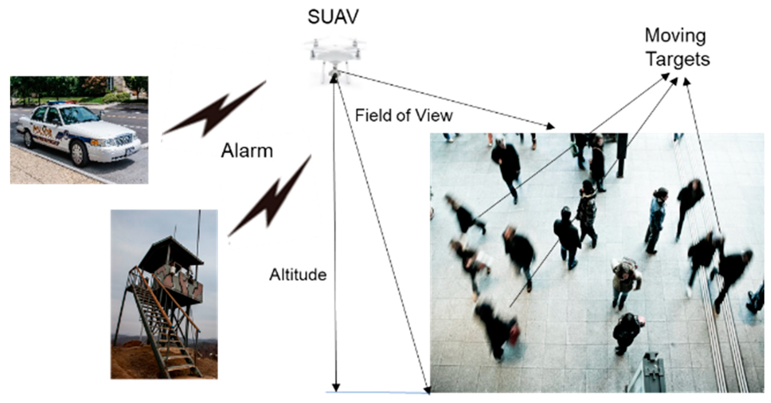
The major contributions of this paper lie in the following: (1) we integrate visual detection based on image processing and a target tracking derived from statistical estimation. In the literature, image-based detection and state estimation-based target tracking are often researched individually, but few studies are found that integrate the two parts. It is noted that we instantly get dynamic state estimates, such as position, velocity, and acceleration, in the proposed method; (2) No massive training data is required for target detection and tracking. Thus, this method can speed up the process, with less computational resources. Drones have limited computing power, memory, bandwidth, and battery; thus, a small computational load is required for a drone system; (3) A practical solution is proposed for autonomous stand-alone aerial surveillance. The SUAV can move to any location where CCTV cameras cannot be installed and hover or maintain its position. It is very low cost and can be operated by non-experts. Thus, it is useful for combat missions, counter terrorist operations, or search and rescue in military or commercial use. Figure 1 illustrates fully autonomous stand-alone aerial video surveillance with an SUAV. The SUAV continuously monitors human movement within the field of view of the attached camera at a certain altitude. If any threat is detected, an alert is sent to the authorities.
2. Object Detection with Frame Subtraction
A current frame is subtracted from a past frame at a constant interval. A thresholding step follows to generate a binary image as:
where I(m,n;k) and I(m,n;k–kd) are the kth frame and the (k–kd)th frame, respectively, kd is a constant interval for frame subtraction, θT is a thresholding value, and M and N are pixel sizes in x and y directions, respectively. After this, a morphological filter, dilation is applied to the binary image to enlarge the segmented regions. The dilation operation is defined as [26]:
where D is the structuring element for dilation, and l denotes an integer value less than the image size. All alternative regions are considered candidate target regions. At last stage of detection, false target regions are removed as:
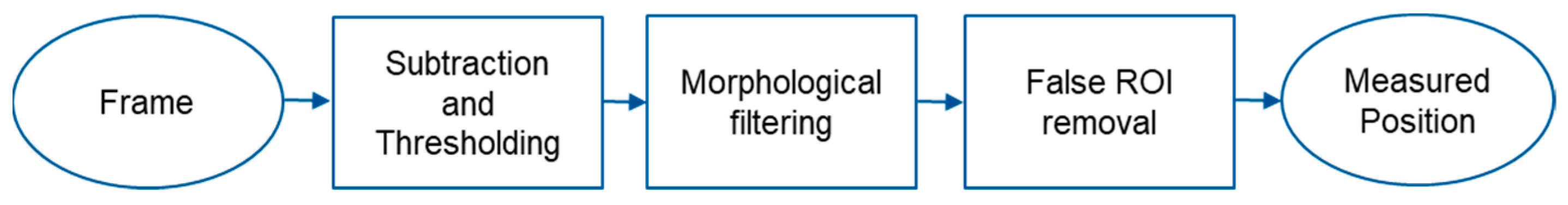
where Oi is the i-th region, θs and θf are the minimum and the maximum size of region, respectively; they are determined based on the true size of the target. The center of each target region is considered a measured position for target tracking in the next section. Figure 2 is the block diagram of moving object detection.
3. Target Tracking with IMM Filtering
3.1. System Modeling
The dynamic state of the target is modeled as a nearly constant velocity (NCV) model; the targets’ maneuvering is modeled by the uncertainty of the process noise, which is assumed to follow the Gaussian distribution. The following is the discrete state equation of target t:
where xt(k) is the state vector of target t at frame k, which is composed of positions and velocities in x and y directions as , T denotes matrix transpose, Δ is the sampling time, v(k) is a process noise vector composed of Gaussian white noise in x and y directions as , is the number of targets at frame k, and F(Δ) and q(Δ) are the transition and the noise gain matrix, respectively. They are defined as:
The filter modes of the IMM filter is set up with different covariance matrices of v as where M is the number of filter modes. The following is the measurement equation of target t:
where is the measurement vector of target t which is composed of positions in x and y directions as , w(k) is a measurement noise vector composed of Gaussian white noise in x and y directions as . It is assumed that the covariance matrix of w(k) is , and H is the measurement matrix, defined as:
3.2. Multi-Mode Interaction
The state vectors and the covariance matrices of the IMM mode filters at the previous frame k−1 are mixed to generate the initial state vectors and the covariance matrices for each of the IMM mode filter at the current frame k:
where and are, respectively, the state vector estimation and the covariance matrix at the previous frame, is the i-th mode probability of target t, and pij is the mode transition probability from mode i to mode j.
3.3. Mode Matched Kalman Filtering
The Kalman filter was performed for each IMM mode. The first step is to predict the state of each target of which the dynamic state is modeled as:
Next, the residual covariance and the filter gain are, respectively, obtained as:
3.4. Measurement Gating and Data Association
Measurement gating is a pre-process of data association that reduces the number of candidate measurements. Let Z(k) be a set of measurement vectors detected at frame k:
where m(k) is the number of measurements at frame k. The measurement gating is chi-squared hypothesis testing, assuming the Gaussian measurement residuals. Thus, a set of valid measurements for target t and mode j is obtained as:
where is the gating size. The NN rule is adopted to associate a measurement with a track by minimizing the norm of the residual as:
and is the number of candidate measurements which falls in the validation region for target t and mode j.
3.5. State Estimate and Covariance Update
The state estimate and the covariance matrix of targets are updated as:
If is equal to zero, i.e., no measurement exists in the validation region, the state estimate and the covariance become the predictions of the state and the covariance as:
The mode probability is updated as:
where N denotes Gaussian probability density function. If no measurement exists in the validation region, the mode probability becomes:
Finally, the state vector and covariance matrix of each target are updated as:
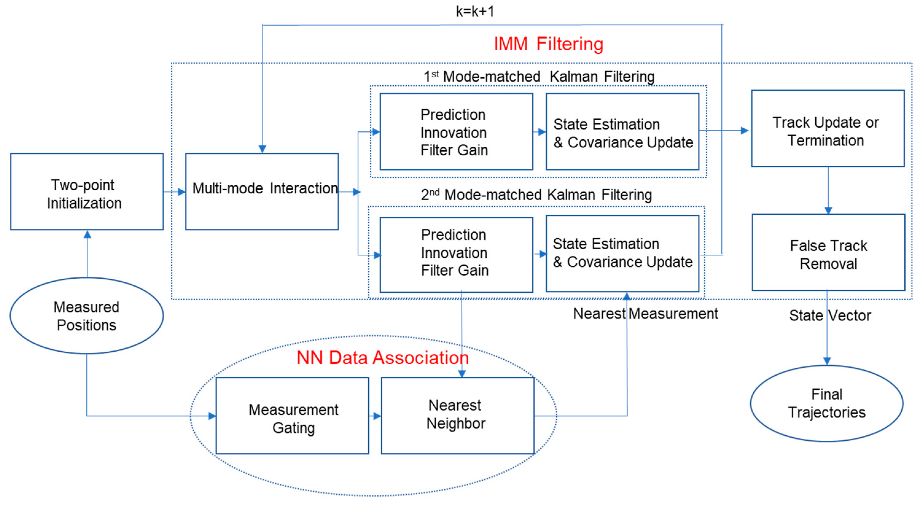
The procedures from Equation (10) to Equation (29) repeat until the track is terminated. Figure 3 is the block diagram of moving object tracking. The track is terminated when the track continuously fails to update its state with validated measurements for a certain number of frames. It is noted that when there is no measurement in the validation region, the track can update its state as Equations (23) and (24), not Equations (21) and (22). The terminated track is also considered false if the number of updates with validated measurements is too small, that is, it is assumed that the true target generates at least a certain number of validated measurements.
3.6. Performance Evaluation
Several metrics are used for performance evaluation, position error, velocity error, and RMSE of position and velocity. The position error of target t at frame k is obtained in x and y directions, respectively:
where and are the ground truth of position of target t in x and y directions, respectively, Nt and Nk are, respectively, the total number of targets and the total number of frames. The ground truth of positions of targets is obtained manually at each scene. The RMSE of position is obtained as:
where Kt(s) and Kt(f) are the first and last frame where target t is estimated. The velocity error of target is obtained in x and y directions, respectively:
where the ground truth of the velocity is approximated as:
where is heuristically set up when the minimum velocity error is produced in the experiments.
The RMSE of velocity is obtained as:
4. Results
4.1. Experimental Set-Up
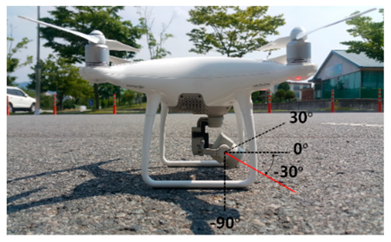
A drone (DJI Phantom 4 Advanced) was used to capture moving objects. The drone, with an attached gimbal and camera, is shown in Figure 4. The gimbal can tilt the camera within a 120° range (−90° to 30°). The camera pitch was set to −30° during the experiments.
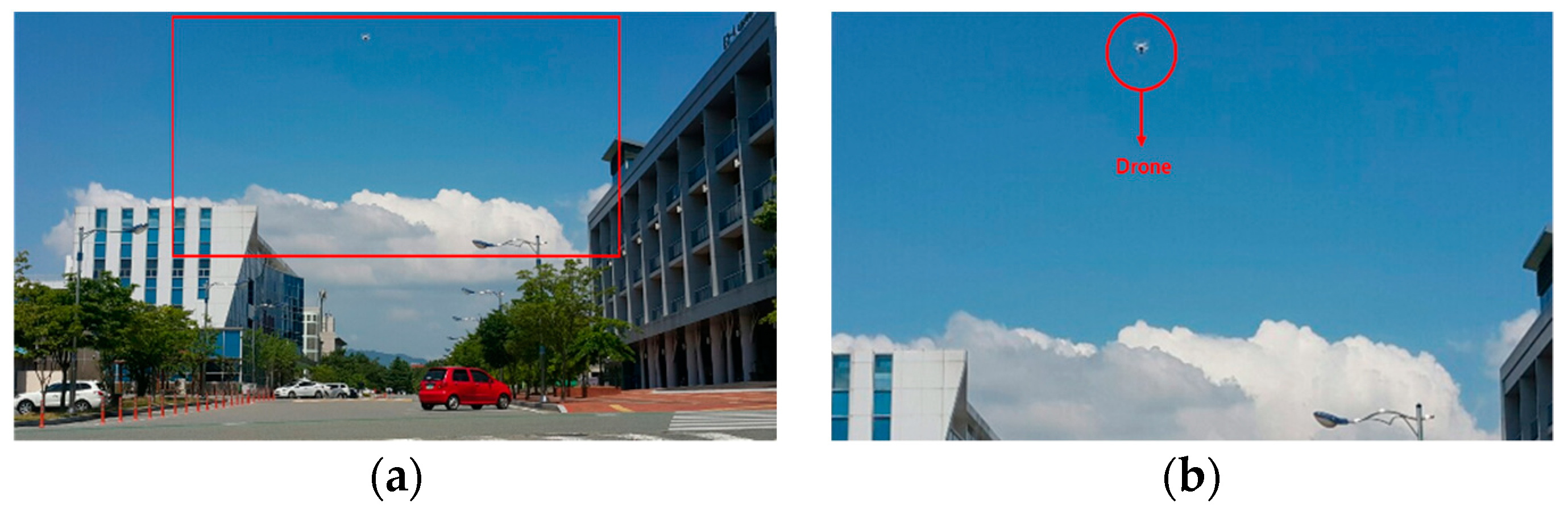
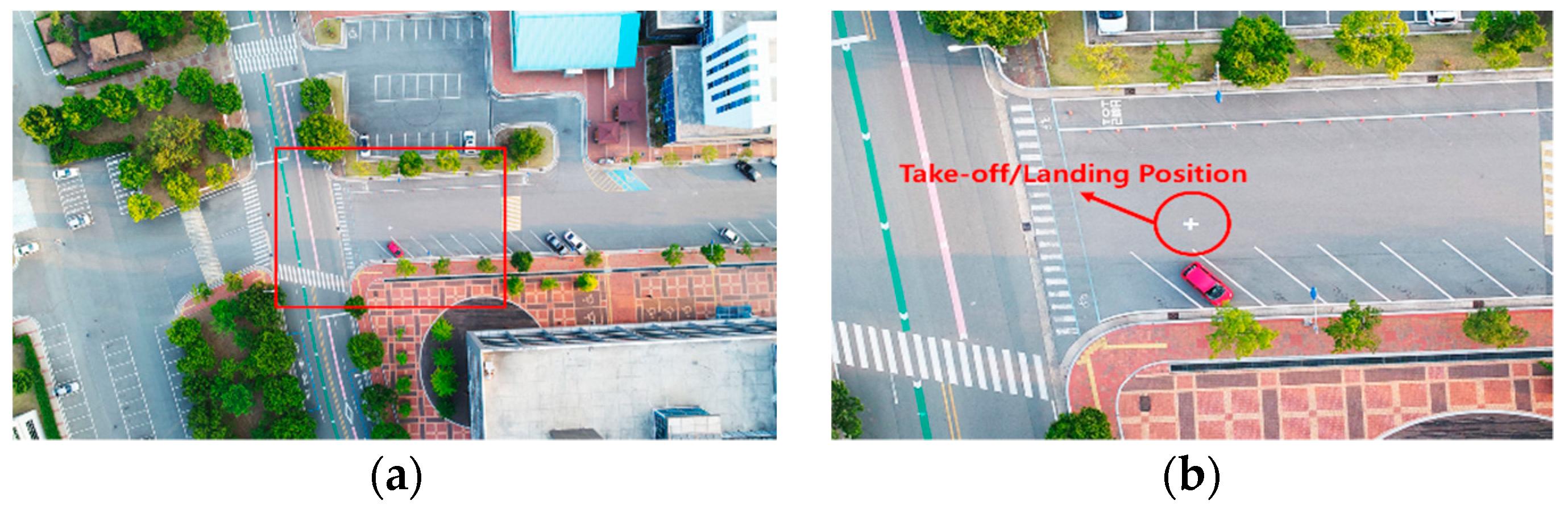
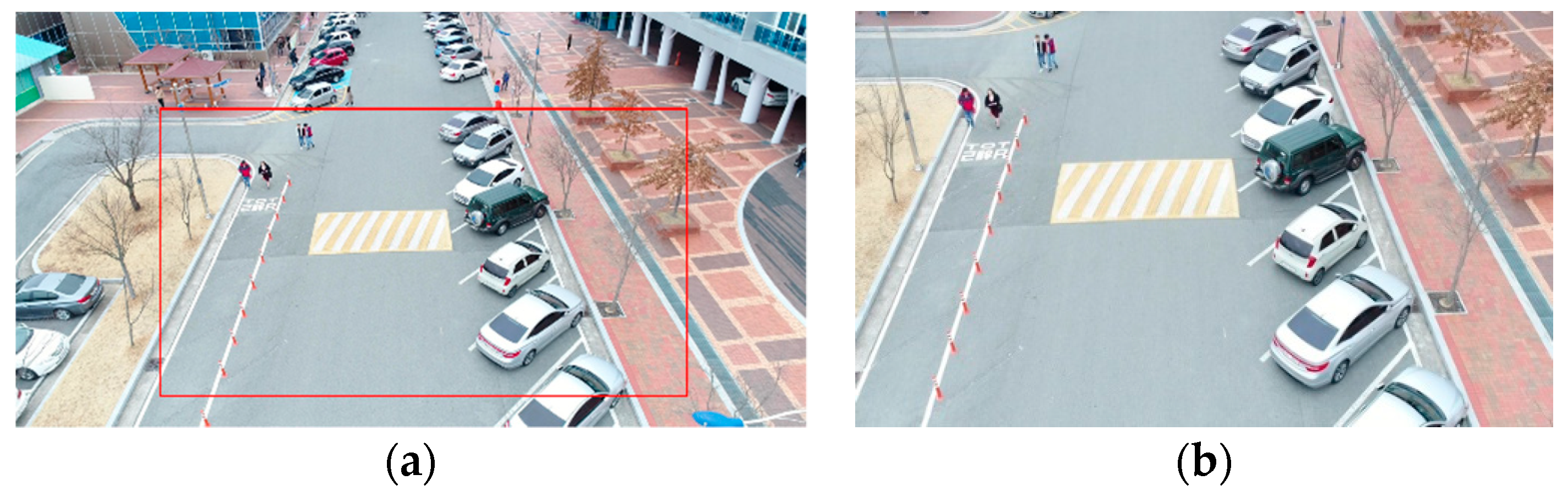
The drone ascended to a height of 15 m and stayed still as a stationary sensor (platform), as shown in Figure 5. It maintained its position while capturing video sequences of moving objects in the campus area. Figure 6 shows the take-off/landing position. Figure 6 was taken by a camera pointing directly downwards (−90° pitch) at a height of 100 m, to better visualize nearby buildings and structures. Figure 7a shows a sample frame extracted from the video. The size of one frame was 4096 × 2160 pixels; the frame was reduced to 20% size for efficient image processing, and the front and central part was cropped to 550 × 300 pixels, as shown in Figure 7b.
4.2. Scenario Description
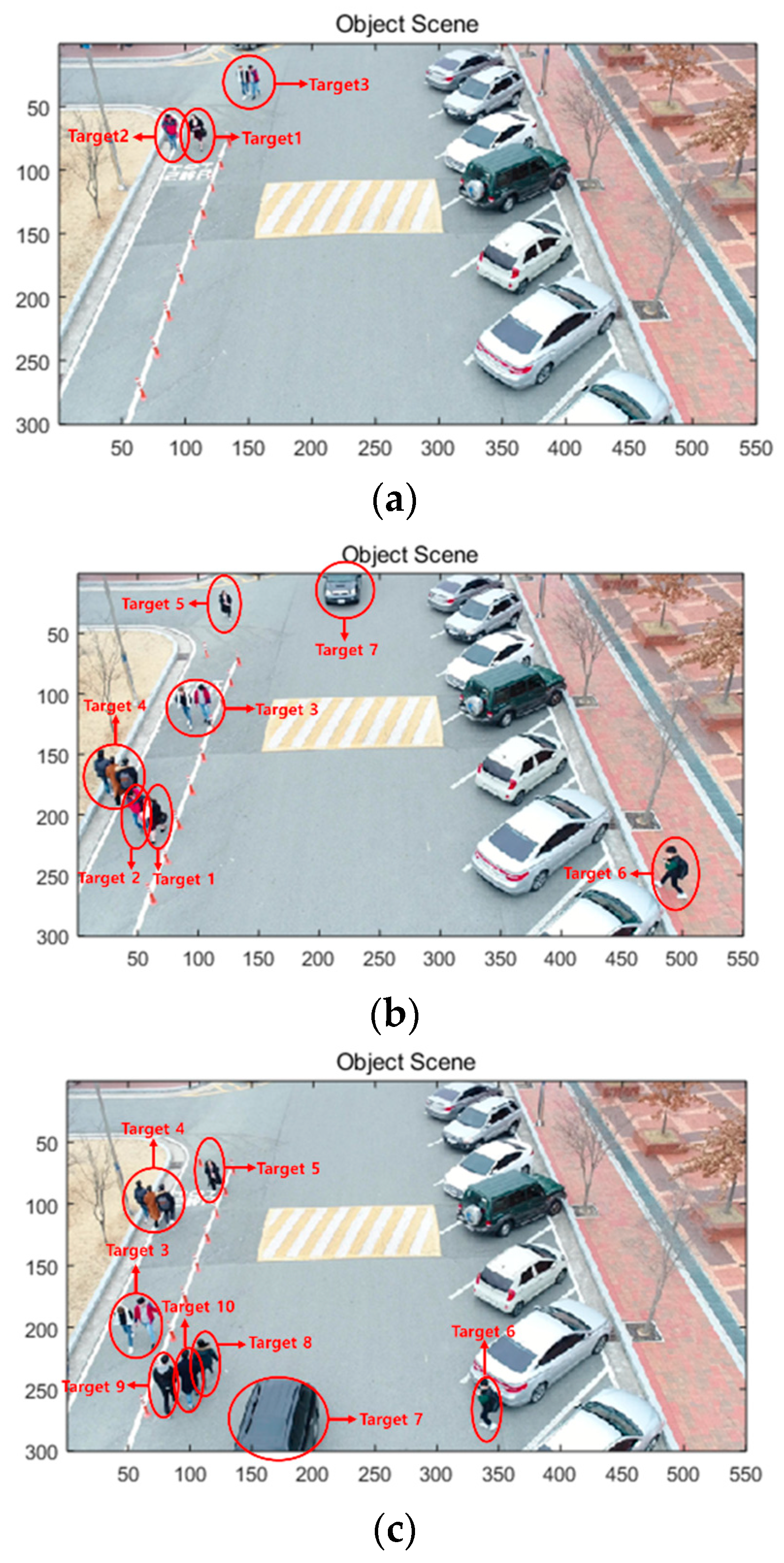
The drone captured a video sequence at 30 frames per second (fps) at a height of 15 m. A total of 13 people and 1 car were captured for 550 frames (16.5 s). Figure 8a shows Targets 1–3 at the sixth frame, Figure 8b shows Targets 1–7 at the 350th frame, and Figure 8c shows Targets 3–10 at the 550th frame. Table 1 shows the duration, moving direction, and components of each target. All targets were composed of one person or one car except for Target 3 and 4, which were composed of two and three people, respectively. Target 1 was partly composed of two people, because the person in Target 2 merged to Target 1 after 237th frame.
4.3. Detection of Moving Objects
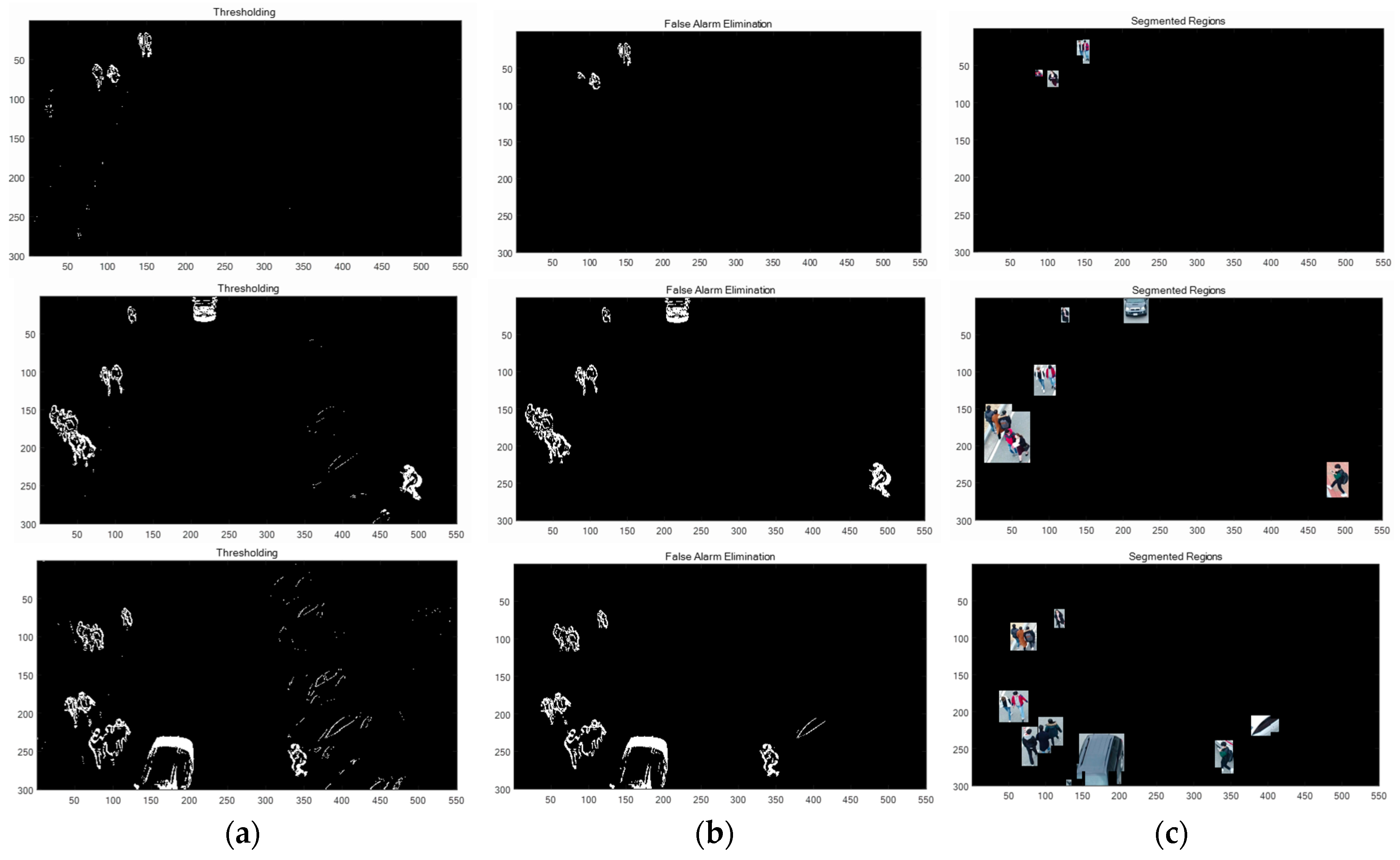
The detection and tracking methods were implemented in MATLAB (version 8.5) on a PC (Intel i5-7500). The interval kd in Equation (1) was set at 5, thus the detection process was applied from the sixth frame; θT in Equation (1) was set at 30; D in Equation (3) was set at , θs and θf in Equation (4) were set at 30 and 1200 pixels, respectively. Figure 9 shows the detection process of the 6th, 350th, and 550th frame. The first row is the detection results of Figure 8a. The second and the third rows are the results of Figure 8b,c, respectively. Figure 9a shows the binary images after the frame subtraction with thresholding. Assuming that the size of the targets is known, Equations (2) and (4) were applied to Figure 9a to result in Figure 9b. Figure 9c shows the target regions with rectangular windows. All targets in three frames were detected, with one false alarm in the 550th frame, as shown in the third row in Figure 9c. Table 2 shows the detection rate of ten targets; the average detection rate was 96.5%. The total number of false alarms detected was 638, thus the false alarm rate was 1.17 per frame. The supplementary material, Video S1: Object Detection (AVI format) for object detection is available online.
4.4. Multiple Target Tracking
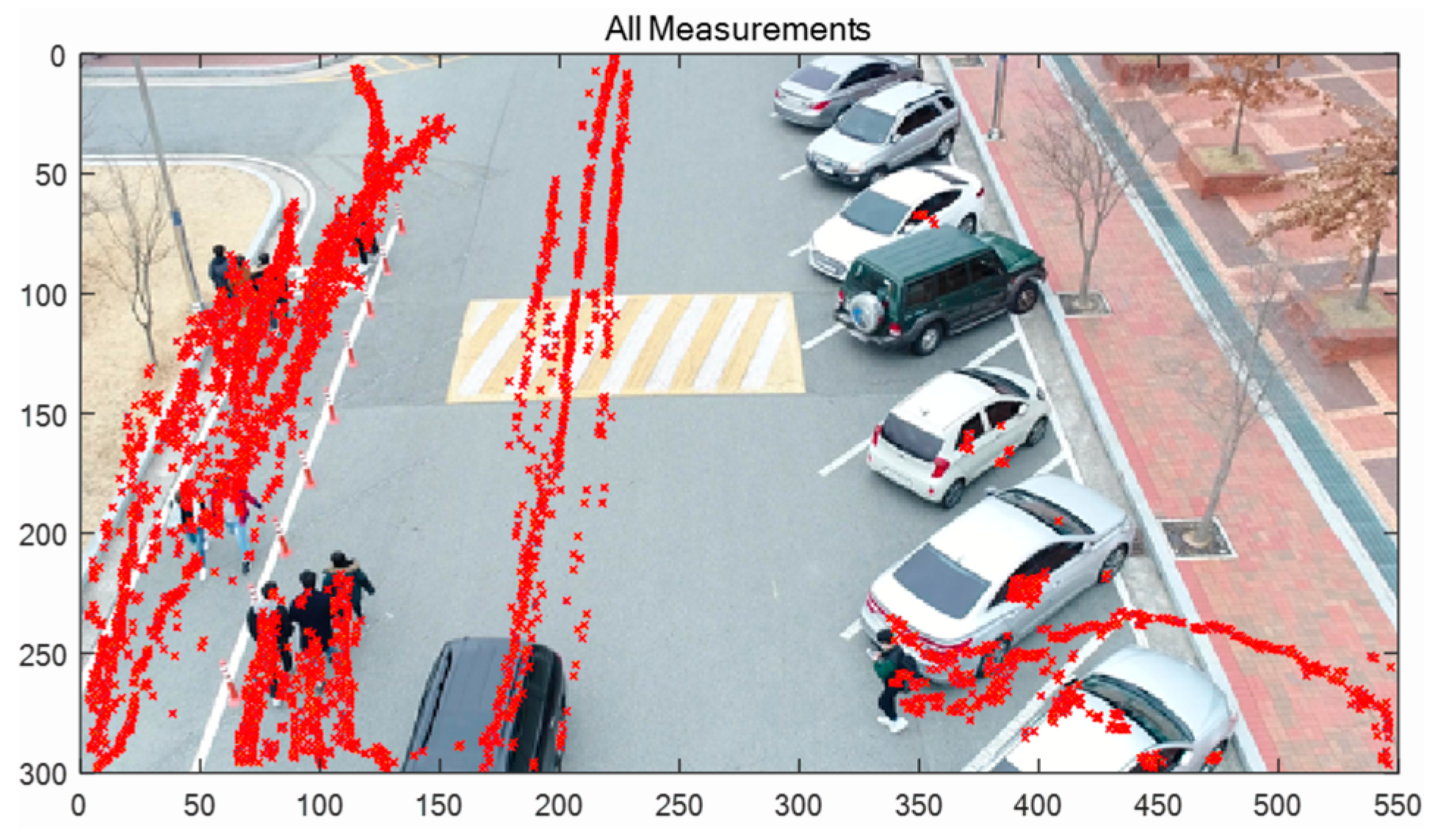
Figure 10 shows all the measured (detected) positions of 10 targets, including false alarms. The sampling time Δ in Equation (5) was 0.033 s, since the frame rate was 30 fps. It was assumed that one pixel corresponds to 0.1 m. The standard deviations of the process and the measurement noise of the two-mode IMM filter were set at , , and , respectively.
For the Kalman filter, , and three-mode IMM filter, , , and ; in Equation (18) for the gating process was set at 8.
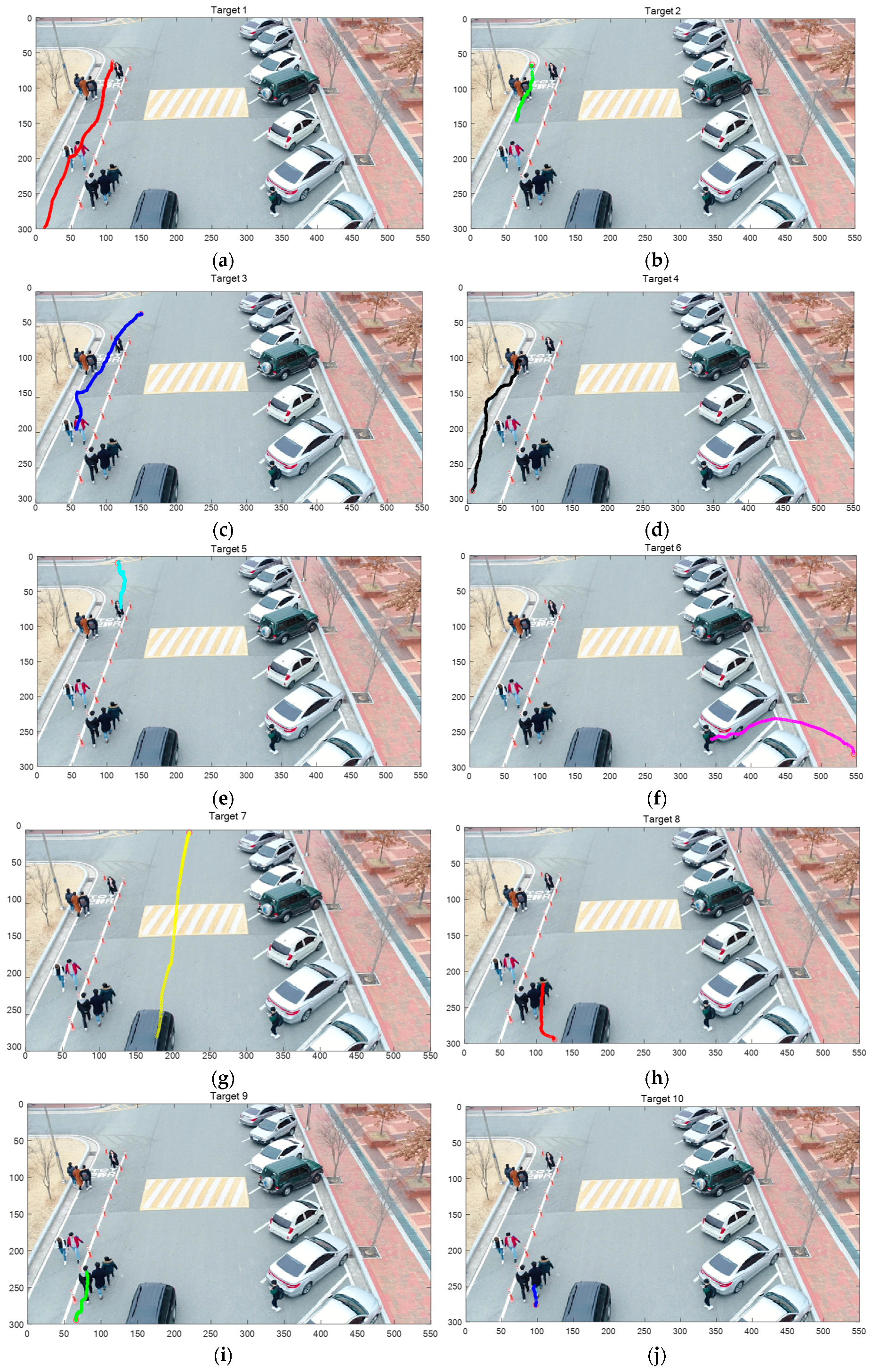
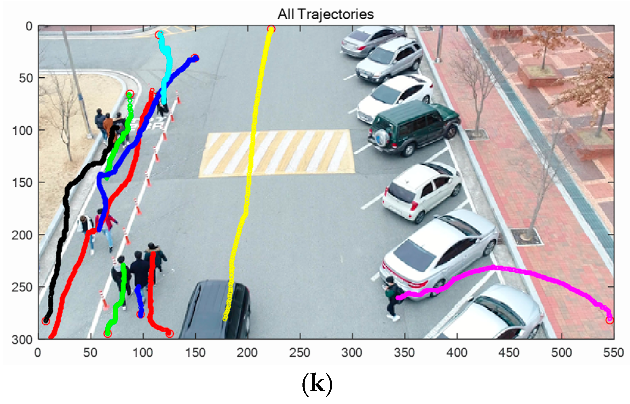
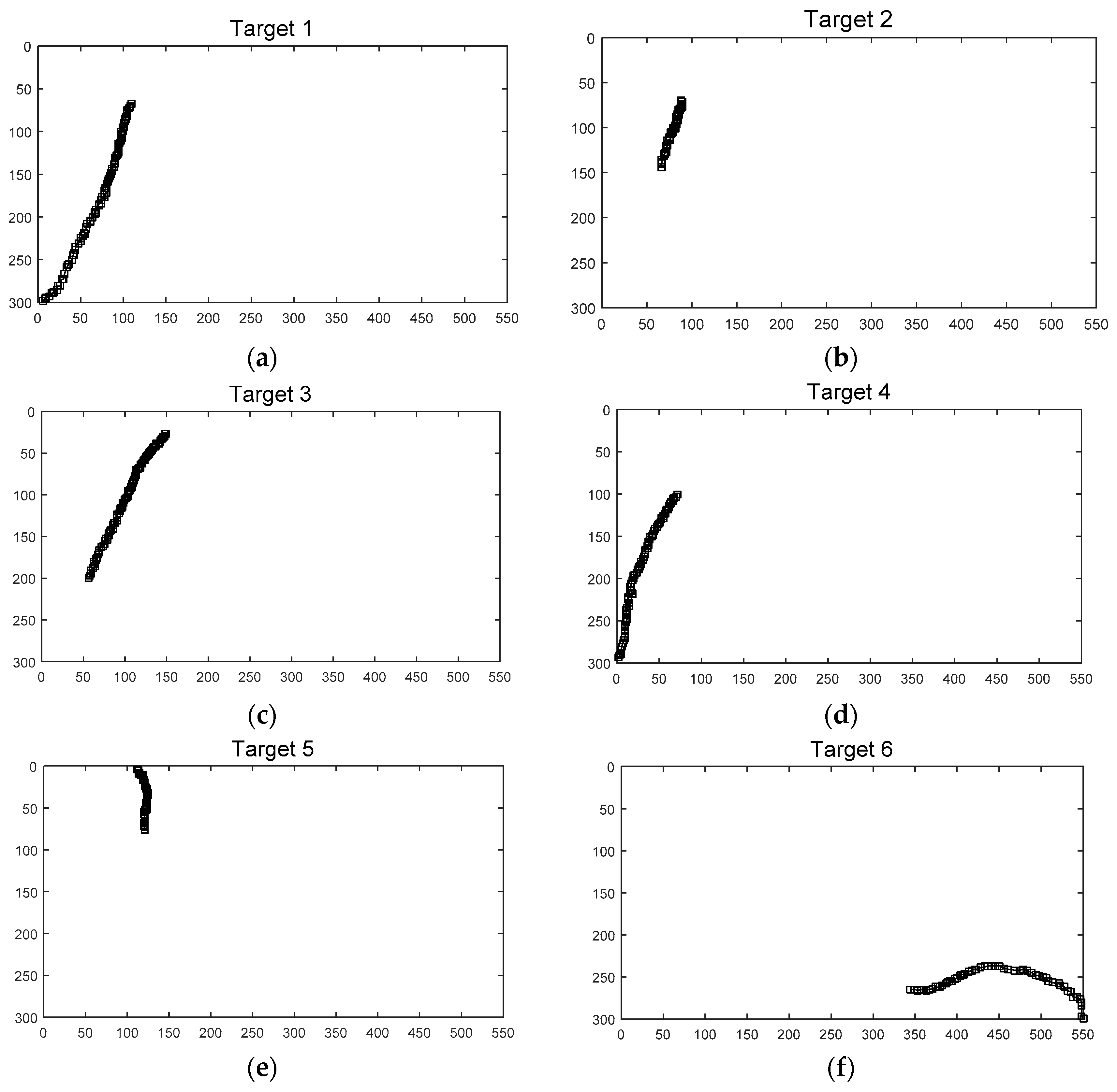
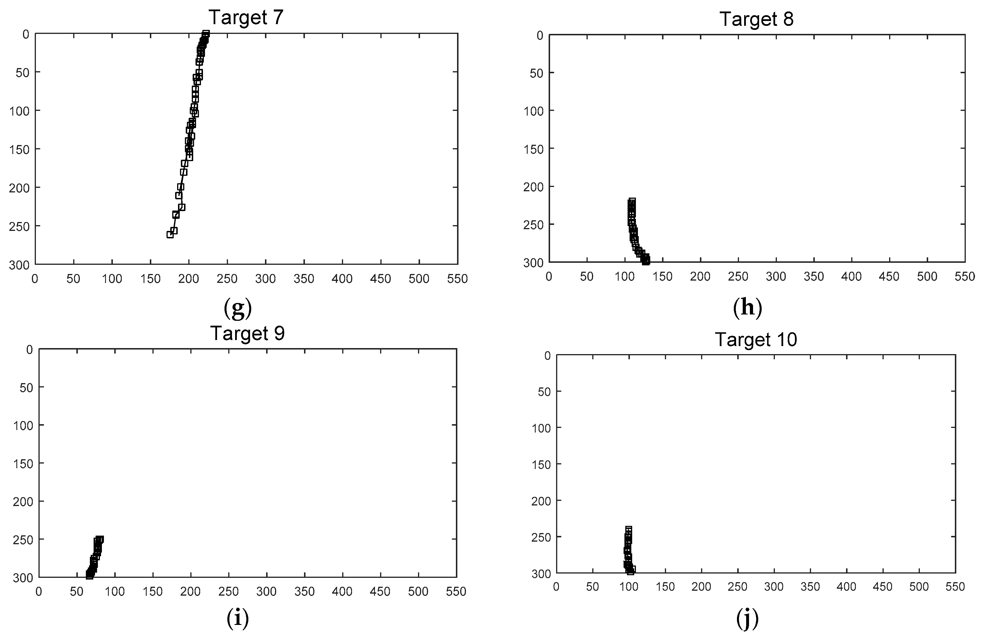
A track was initialized by a two-point initialization method with the speed gating, which limited the maximum speed to 1 m/s. Figure 11a–j are the tracking results of Targets 1–10, respectively. Figure 11k shows all trajectories in one frame. Also, the supplementary material, Video S2: Human Tracking (AVI format) for target tracking is available online. The track was terminated if there were no updates for more than 40 consecutive frames. After termination, the track was considered false if the number of updates with validated measurements was less than 60 times, thus, the true target should be detected in at least 60 frames (2 s).
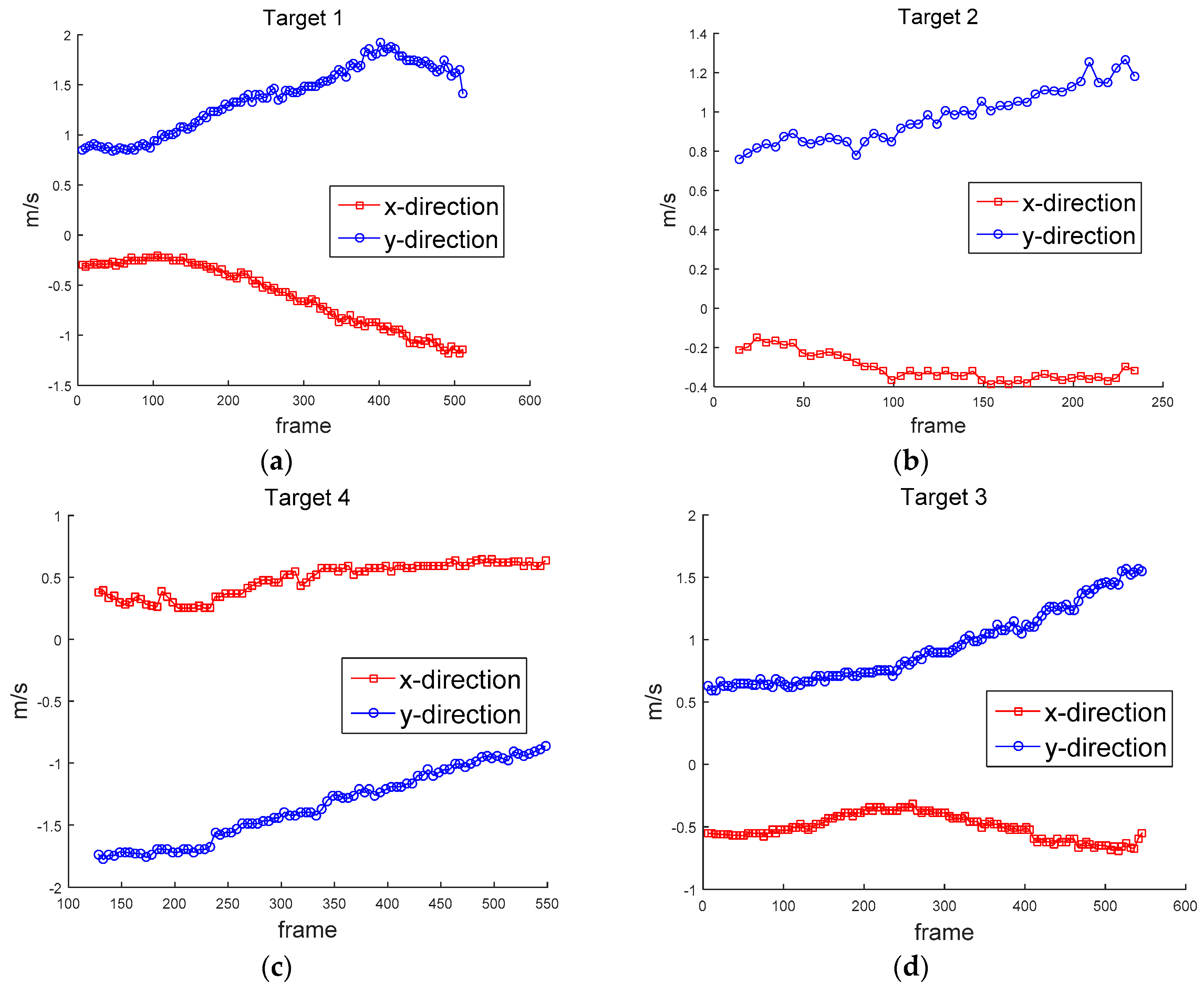
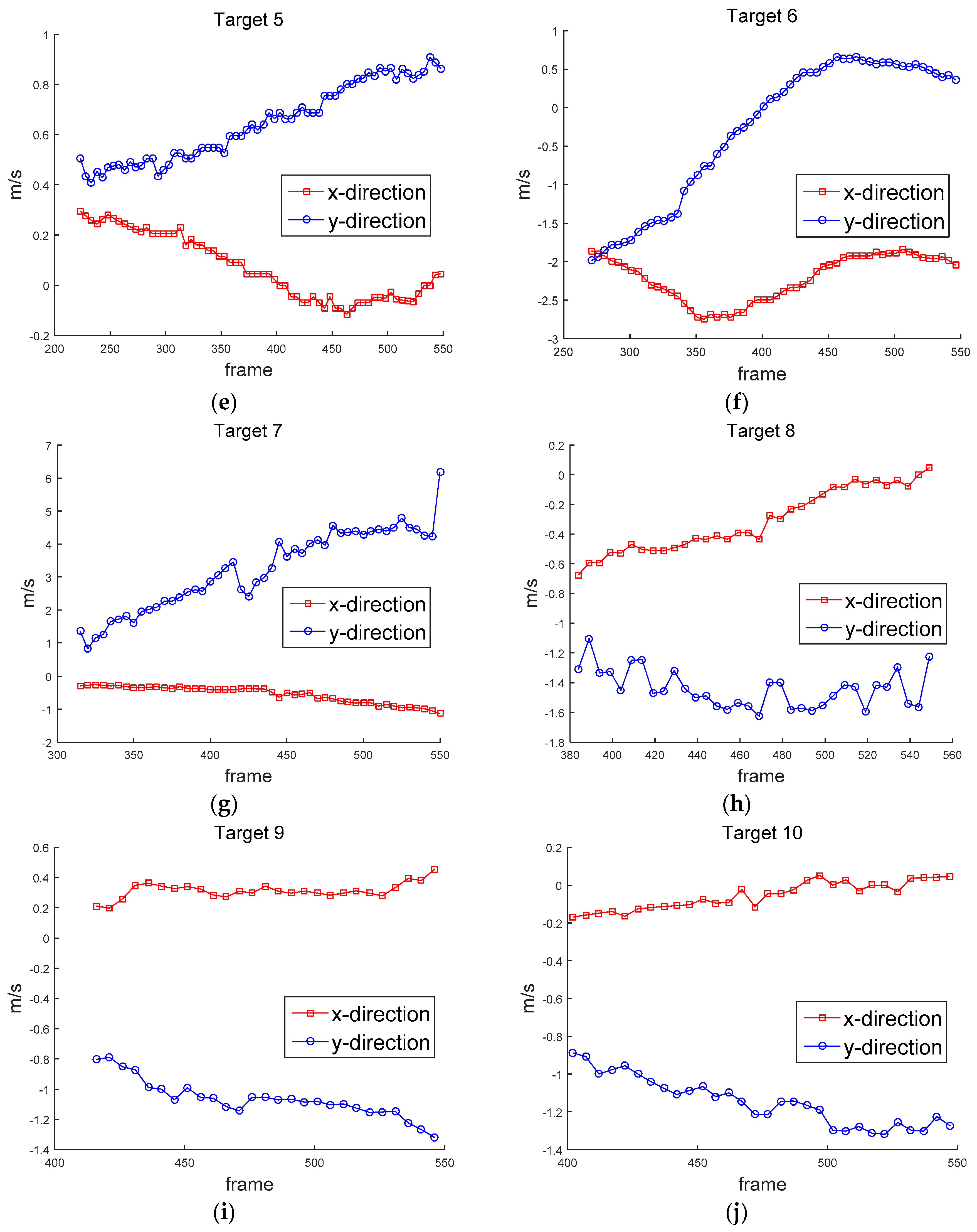
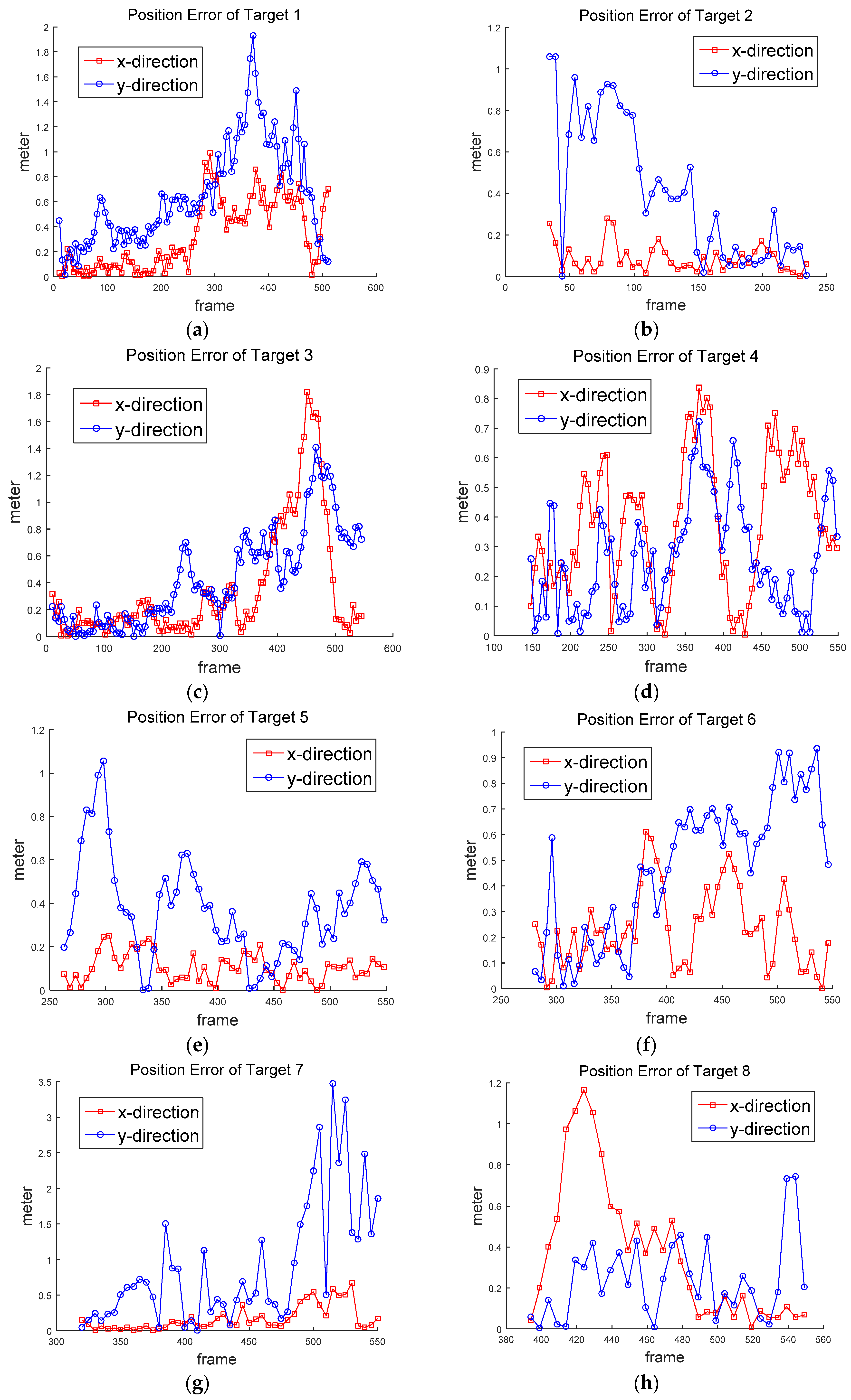
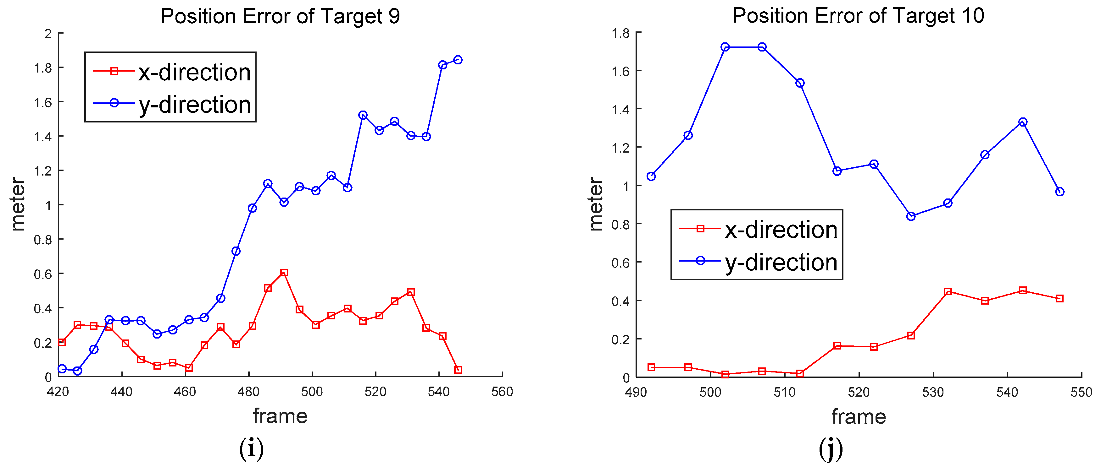
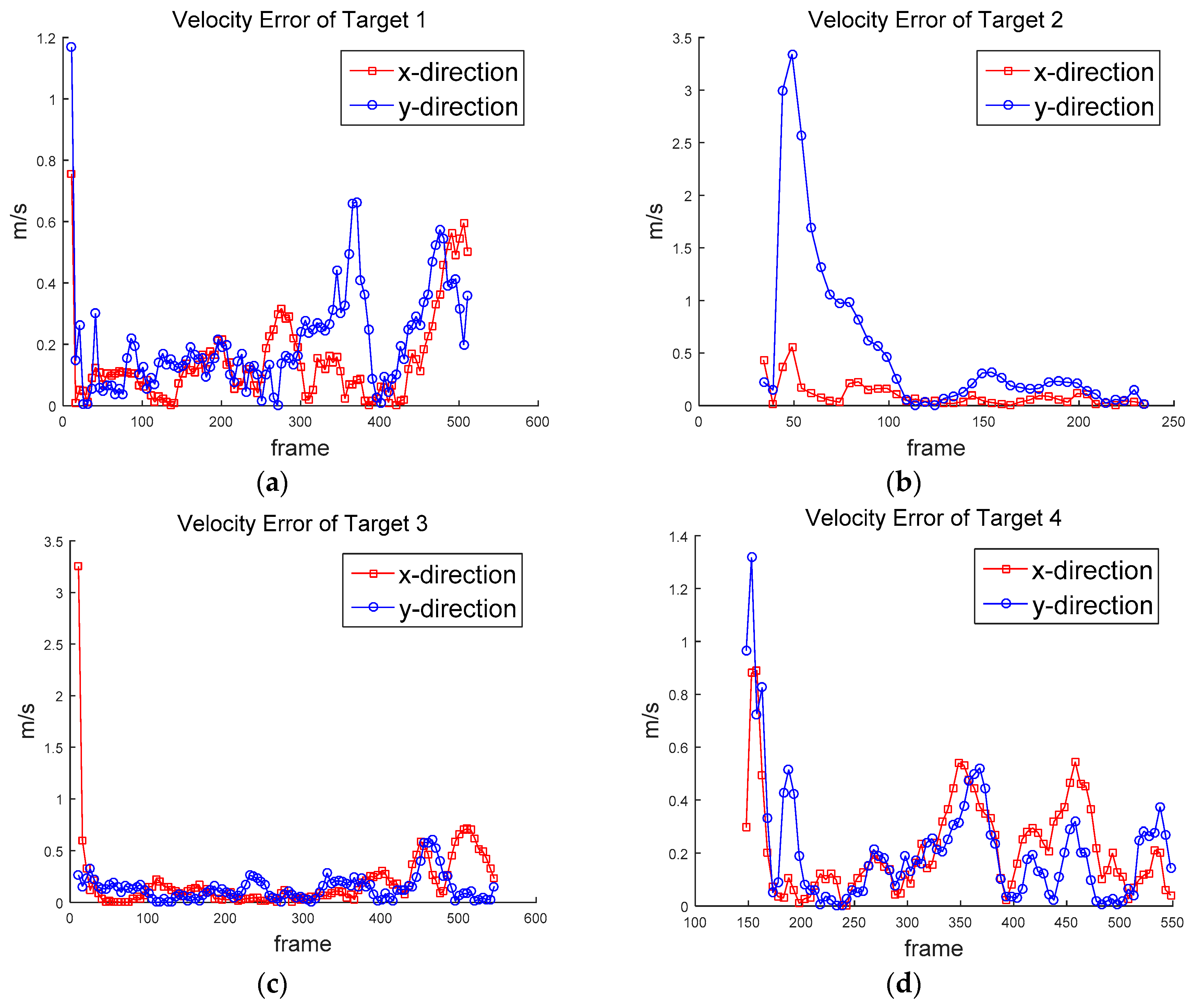
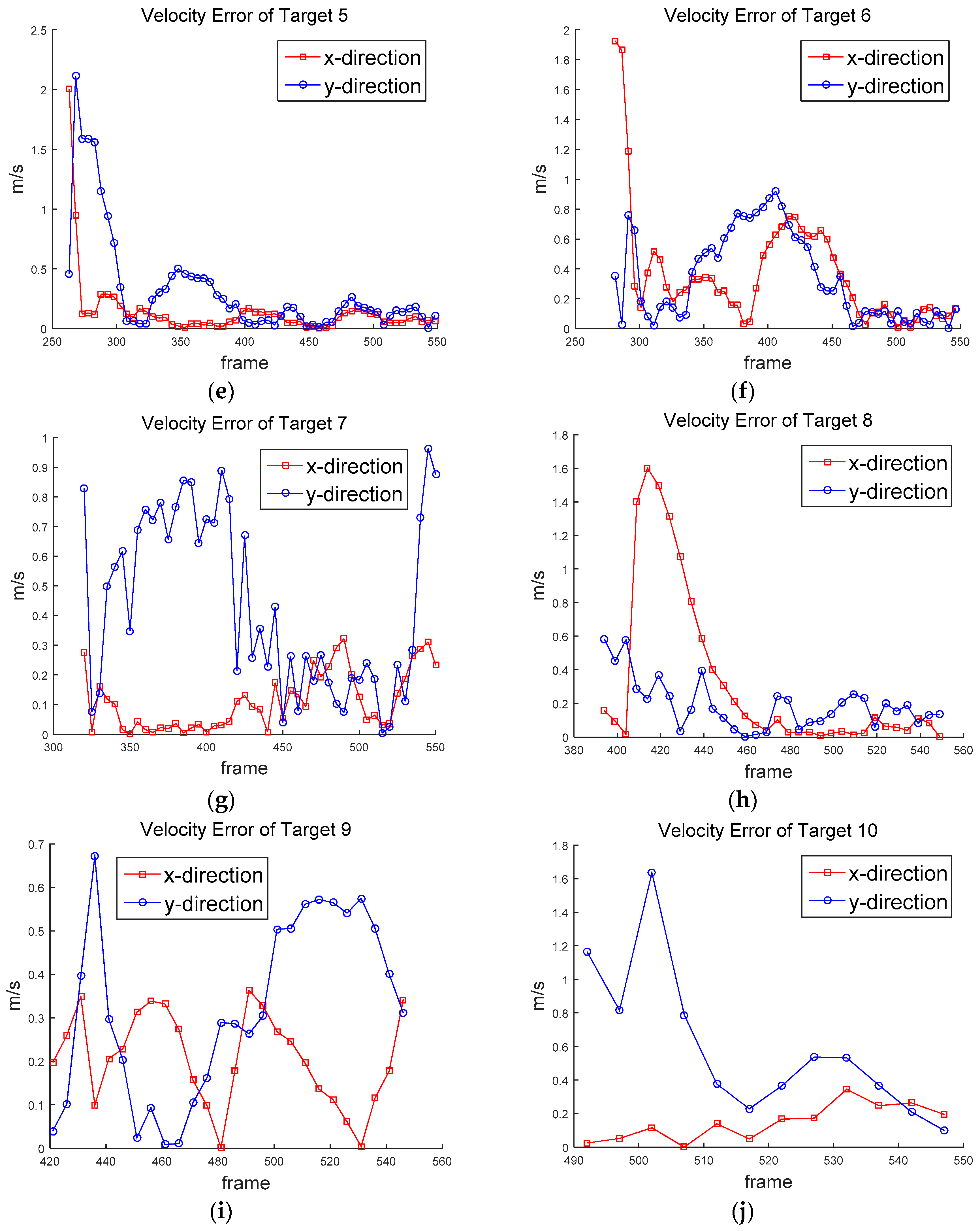
Figure 12 shows the ground truth of the position of the targets. Figure 13 shows the approximated ground truth of the velocity in x and y directions, obtained by Equation (33); was set at 65 when the least average velocity RMSE was produced. Figure 14 and Figure 15 show the position in Equation (30) and velocity errors in Equation (32), respectively.
Table 3 shows the RMSE of position and velocity obtained in Equations (31) and (34), respectively.
5. Discussion
Table 2 shows the detection rates of ten targets—the average detection rate was 96.5%. The detection rate of Target 5 was particularly low, at 74.5%. Target 5 was located far away from the drone, as shown in Figure 8b and Figure 11e. Therefore, its relative lower speed caused detection to be missed during frame subtraction. The false alarm rate was 1.17 per frame. The false alarms were mostly generated when the drone was swung by the wind or the objects passed through a complex background. Table 3 shows the RMSE of position and velocity. The average RMSE of the position was about 0.8 m, and the average RMSE of the velocity was about 0.586 m/s (≈2.1 km/h) for the two-mode IMM filter. The minimum RMSEs were obtained when the two-mode IMM filter was used. It turns out that the process noise standard deviations (0.6 and 1 m/s2) were properly chosen, because similar results were obtained from the Kalman filter with the average standard deviation (0.8 m/s2). The two-mode IMM filter provided slightly better results than the Kalman filter. It was especially good for Target 7 (car), which moved to higher maneuvers than other targets. It is noted that the IMM filter with three modes did not provide better results in this scenario.
The position RMSE varied from 0.458 m for Target 5 to 1.284 m for Target 10. The average RMSE (about 0.8 m) was close to half the human height. Except for Target 7 (car), Targets 9 and 10 generated higher position errors than other targets; there were biases between the measurements and the position estimates. The velocity RMSE varied from 0.342 m/s (1.23 km/h) for Target 1 to 0.959 m/s for Target 2 (3.45 km/h). The speed of human movement is important because we can recognize the threats from unexpected movements.
6. Conclusions
In this paper, several moving people and cars were captured by an SUAV. The objects were detected based on frame subtraction. Ten targets were tracked with the Kalman and IMM filters. Experimental results show that moving objects were well detected and tracked with good accuracy. The number of filter modes and the target dynamics of each mode, such as the process noise variance, should be determined properly to cope with the maneuvering of multiple targets.
For security and defense applications, the trajectories and the states of targets can be transferred to a control tower in real-time. Also, this system is suitable for people counting in a crowd area. Fully autonomous and stand-alone aerial video surveillance systems are very useful in commercial as well as military/government applications. In this work, the drone was fixed in the air as a stationary sensor (platform). Target tracking with a moving platform remains a subject for future study.
Supplementary Materials
The following are available online at https://0-www-mdpi-com.brum.beds.ac.uk/2076-3417/9/16/3359/s1, Video S1: Object Detection, Video S2: Human Tracking.
Author Contributions
Conceptualization, methodology, software, validation, S.Y.; and visualization and experimental assistance, I.-J.C.
Funding
This research was supported by Basic Science Research Program through the National Research Foundation of Korea (NRF) funded by the Ministry of Education (Grant Number: 2017R1D1A3B03031668).
Conflicts of Interest
The authors declare no conflict of interest.
References
- 2015 FAA Operation and Certification of Small Unmanned Aircraft Systems. Available online: https://www.faa.gov/regulations_policies/rulemaking/recently_published/media/2120-AJ60_NPRM_2-15-2015_joint_signature.pdf (accessed on 12 August 2019).
- Kumar, R.; Sawhney, H.; Samarasekera, S.; Hsu, S.; Tao, H.; Guo, Y.L.; Hanna, K.; Pope, A.; Wildes, R.; Hirvonen, D.; et al. Aerial video surveillance and exploitation. Proc. IEEE 2001, 89, 1518–1539. [Google Scholar] [CrossRef]
- Wu, Y.; He, X.; Nguyen, T.Q. Moving object detection with a freely moving camera via background motion subtraction. IEEE Trans. Circ. Syst. Video Technol. 2017, 27, 236–248. [Google Scholar] [CrossRef]
- Zhang, Y.; Huang, X.; Li, J.; Liu, X.; Zhang, H.; Xing, X. Research of moving object detection algorithm in transmission lines under complex background. In Proceedings of the International Conference on Condition Monitoring and Diagnosis, Xi’an, China, 25–28 October 2016; Volume 30, pp. 176–179. [Google Scholar]
- Olugboja, A.; Wang, Z. Detection of moving objects using foreground detector and improved morphological filter. In Proceedings of the 2016 3rd International Conference on Information Science and Control Engineering, Vienna International Hotels, Beijing, China, 8–10 July 2016. [Google Scholar]
- Yeom, S.; Lee, M.H.; Cho, I.J. Long-range moving object detection based on background subtraction. In Proceedings of the 18th International Symposium on Advanced Intelligent Systems, Daegu, South Korea, 11–14 October 2017; pp. 1082–1085. [Google Scholar]
- Smeulders, A.W.M.; Chu, D.M.; Cucchiara, R.; Calderara, S.; Dehghan, A.; Shah, M. Visual tracking: An experimental survey. IEEE Trans. Pattern Anal. Mach. Intell. 2014, 36, 1442–1468. [Google Scholar]
- Park, S.M.; Park, J.; Kim, H.B.; Sim, K.B. Specified object tracking problem in an environment of multiple moving objects. Int. J. Fuzzy Log. Intell. Syst. 2011, 11, 118–123. [Google Scholar] [CrossRef]
- Feng, X.; Mei, W.; Hu, D. A review of visual tracking with deep learning. Adv. Intell. Syst. Res. 2016, 133, 231–234. [Google Scholar]
- Yun, S.; Choi, J.; Yoo, Y.; Yun, K.; Choi, J.Y. Action-decision networks for visual tracking with deep reinforcement learning. In Proceedings of the IEEE Conference on CVPR2017, Honolulu, HI, USA, 21–26 July 2017; pp. 2711–2720. [Google Scholar]
- Li, P.; Wang, D.; Wang, L.; Lu, H. Deep visual tracking: Review and experimental comparison. Pattern Recognit. 2018, 76, 323–338. [Google Scholar] [CrossRef]
- Chen, P.; Dang, Y.; Liang, R.; Zhu, W.; He, X. Real-time object tracking on a drone with multi-inertial sensing data. IEEE Trans. Intell. Trans. Syst. 2018, 19, 131–139. [Google Scholar] [CrossRef]
- Bian, C.; Yang, Z.; Zhang, T.; Xiong, H. Pedestrian tracking from an unmanned aerial vehicle. In Proceedings of the 2016 IEEE 13th International Conference on Signal Processing (ICSP), Chengdu, China, 6–10 November 2016; pp. 1067–1071. [Google Scholar]
- Risse, B.; Mangan, M.; del Pero, L.; Webb, B. Visual tracking of small animals in cluttered natural environments using a freely moving camera. In Proceedings of the 2017 IEEE International Conference on Computer Vision Workshops, Venice, Italy, 22–29 October 2017; pp. 2840–2849. [Google Scholar]
- Kim, J.; Kim, Y. Moving ground target tracking in dense obstacle areas using UAVs. IFAC Proc. Vol. 2008, 41, 8552–8557. [Google Scholar] [CrossRef] [Green Version]
- Yeom, S.; Kirubarajan, T.; Bar-Shalom, Y. Track segment association, fine-step IMM and initialization with Doppler for improved track performance. IEEE Trans. Aerosp. Electron. Syst. 2004, 40, 293–309. [Google Scholar] [CrossRef]
- Stone, L.D.; Streit, R.L.; Corwin, T.L.; Bell, K.L. Bayesian Multiple Target Tracking, 2nd ed.; Artech House: Boston, MA, USA, 2014. [Google Scholar]
- Blom, H.A.P.; Bar-shalom, Y. The interacting multiple model algorithm for systems with Markovian switching coefficients. IEEE Trans. Autom. Control 1988, 33, 780–783. [Google Scholar] [CrossRef]
- Zhou, H.; Zhao, H.; Huang, H.; Zhao, X. A Cubature-principle-assisted IMM-adaptive UKF algorithm for maneuvering target tracking caused by sensor faults. Appl. Sci. 2017, 7, 3. [Google Scholar] [CrossRef]
- Li, T.; Su, J.; Liu, W.; Corchado, J.M. Approximate Gaussian conjugacy: Parametric recursive filtering under nonlinearity, multimodality, uncertainty, and constraint, and beyond. Front. Inform. Technol. Electron. Eng. 2017, 18, 1913–1939. [Google Scholar] [CrossRef]
- Bar-Shalom, Y.; Li, X.R. Multitarget-Multisensor Tracking: Principles and Techniques; YBS Publishing: Storrs, CT, USA, 1995. [Google Scholar]
- Reid, D.B. An algorithm for tracking multiple targets. IEEE Trans. Autom. Control 1979, 24, 843–854. [Google Scholar] [CrossRef]
- Deb, S.; Yeddanapudi, M.; Pattipati, K.R.; Bar-Shalom, Y. A generalized S-D assignment algorithm formultisensor-multitarget state estimation. IEEE Trans. Aerosp. Electron. Syst. 1997, 33, 523–538. [Google Scholar]
- Lee, M.H.; Yeom, S. Detection and tracking of multiple moving vehicles with a UAV. Int. J. Fuzzy Log. Intell. Syst. 2018, 18, 182–189. [Google Scholar] [CrossRef]
- Lee, M.H.; Yeom, S. Multiple target detection and tracking on urban roads with a drone. J. Intell. Fuzzy Syst. 2018, 35, 6071–6078. [Google Scholar] [CrossRef]
- Gonzalez, R.C.; Woods, R.E. Digital Image Processing, 4th ed.; Pearson: New York, NY, USA, 2017. [Google Scholar]
Figure 1.
Illustration of aerial surveillance with a small unmanned aerial vehicle (SUAV).

Figure 2.
Block diagram of moving object detection.

Figure 3.
Block diagram of moving object tracking.

Figure 4.
Drone with an attached camera.

Figure 5.
(a) Picture of a drone at a height of 15 m, (b) magnification of Figure 5a.
Figure 5.
(a) Picture of a drone at a height of 15 m, (b) magnification of Figure 5a.

Figure 6.
(a) Picture of a take-off/landing position, (b) magnification of Figure 6a.
Figure 6.
(a) Picture of a take-off/landing position, (b) magnification of Figure 6a.

Figure 7.
(a) Sample frame (4096 × 2160 pixels), (b) cropped region after resizing (550 × 300 pixels).
Figure 7.
(a) Sample frame (4096 × 2160 pixels), (b) cropped region after resizing (550 × 300 pixels).

Figure 8.
(a) Targets 1–3 in the sixth frame, (b) Targets 1–7 in the 350th frame, (c) Targets 3–10 in the 550th frame.
Figure 8.
(a) Targets 1–3 in the sixth frame, (b) Targets 1–7 in the 350th frame, (c) Targets 3–10 in the 550th frame.

Figure 9.
(a) Frame subtraction with thresholding, (b) morphological filtering and false region removal, (c) target region windows.
Figure 9.
(a) Frame subtraction with thresholding, (b) morphological filtering and false region removal, (c) target region windows.

Figure 10.
Measured positions, including false alarms.

Figure 11.
Tracking results, (a) Target 1, (b) Target 2, (c) Target 3, (d) Target 4, (e) Target 5, (f) Target 6, (g) Target 7, (h) Target 8, (i) Target 9, (j) Target 10, (k) All Targets.
Figure 11.
Tracking results, (a) Target 1, (b) Target 2, (c) Target 3, (d) Target 4, (e) Target 5, (f) Target 6, (g) Target 7, (h) Target 8, (i) Target 9, (j) Target 10, (k) All Targets.


Figure 12.
Ground truth of position, (a) Target 1, (b) Target 2, (c) Target 3, (d) Target 4, (e) Target 5, (f) Target 6, (g) Target 7, (h) Target 8, (i) Target 9, (j) Target 10.
Figure 12.
Ground truth of position, (a) Target 1, (b) Target 2, (c) Target 3, (d) Target 4, (e) Target 5, (f) Target 6, (g) Target 7, (h) Target 8, (i) Target 9, (j) Target 10.


Figure 13.
Ground truth of velocity in x and y directions, (a) Target 1, (b) Target 2, (c) Target 3, (d) Target 4, (e) Target 5, (f) Target 6, (g) Target 7, (h) Target 8, (i) Target 9, (j) Target 10.
Figure 13.
Ground truth of velocity in x and y directions, (a) Target 1, (b) Target 2, (c) Target 3, (d) Target 4, (e) Target 5, (f) Target 6, (g) Target 7, (h) Target 8, (i) Target 9, (j) Target 10.


Figure 14.
Position error of (a) Target 1, (b) Target 2, (c) Target 3, (d) Target 4, (e) Target 5, (f) Target 6, (g) Target 7, (h) Target 8, (i) Target 9, (j) Target 10.
Figure 14.
Position error of (a) Target 1, (b) Target 2, (c) Target 3, (d) Target 4, (e) Target 5, (f) Target 6, (g) Target 7, (h) Target 8, (i) Target 9, (j) Target 10.


Figure 15.
Velocity error of (a) Target 1, (b) Target 2, (c) Target 3, (d) Target 4, (e) Target 5, (f) Target 6, (g) Target 7, (h) Target 8, (i) Target 9, (j) Target 10.
Figure 15.
Velocity error of (a) Target 1, (b) Target 2, (c) Target 3, (d) Target 4, (e) Target 5, (f) Target 6, (g) Target 7, (h) Target 8, (i) Target 9, (j) Target 10.


Table 1.
Target characteristics.
| Target No. | First Frame | Last Frame | Direction | Component |
|---|---|---|---|---|
| Target 1 | 1 | 515 | Downward | 1–2 person(s) |
| Target 2 | 1 | 237 | Downward | 1 person |
| Target 3 | 1 | 550 | Downward | 2 people |
| Target 4 | 123 | 550 | Upward | 3 people |
| Target 5 | 218 | 550 | Downward | 1 person |
| Target 6 | 266 | 550 | Left | 1 person |
| Target 7 | 310 | 550 | Downward | 1 Car |
| Target 8 | 379 | 550 | Upwards | 1 person |
| Target 9 | 411 | 550 | Upwards | 1 person |
| Target 10 | 397 | 550 | Upwards | 1 person |
Table 2.
Detection results.
| Target No | Initial Frame | Final Frame | # of Frames | # of Detection | Detection Rate (%) |
|---|---|---|---|---|---|
| Target 1 | 6 | 515 | 510 | 510 | 100% |
| Target 2 | 6 | 237 | 232 | 230 | 99% |
| Target 3 | 6 | 550 | 545 | 545 | 100% |
| Target 4 | 128 | 550 | 423 | 423 | 100% |
| Target 5 | 223 | 550 | 328 | 242 | 74% |
| Target 6 | 271 | 550 | 280 | 280 | 100% |
| Target 7 | 315 | 550 | 236 | 236 | 100% |
| Target 8 | 384 | 550 | 167 | 167 | 100% |
| Target 9 | 416 | 550 | 135 | 130 | 96% |
| Target 10 | 402 | 550 | 149 | 143 | 96% |
| Avg. | - | - | 326 | 316 | 96.5% |
Table 3.
Root-mean squared errors (RMSE) of position and velocity.
| Target No. | Kalman Filter | Two-Mode IMM Filter | Three-Mode IMM Filter | |||
|---|---|---|---|---|---|---|
| Position (Meter) | Velocity (m/s) | Position (Meter) | Velocity (m/s) | Position (Meter) | Velocity (m/s) | |
| Target 1 | 0.8833 | 0.3412 | 0.8839 | 0.3419 | 0.8827 | 0.3419 |
| Target 2 | 0.5420 | 0.9592 | 0.5428 | 0.9589 | 0.5412 | 0.9589 |
| Target 3 | 0.7956 | 0.4418 | 0.7958 | 0.4466 | 0.8033 | 0.4466 |
| Target 4 | 0.5460 | 0.4186 | 0.5429 | 0.4162 | 0.5563 | 0.4290 |
| Target 5 | 0.4543 | 0.6297 | 0.4547 | 0.6295 | 0.4540 | 0.6299 |
| Target 6 | 0.6071 | 0.6922 | 0.6105 | 0.6941 | 0.6039 | 0.6904 |
| Target 7 | 1.2829 | 0.5496 | 1.2786 | 0.5476 | 1.2871 | 0.5493 |
| Target 8 | 0.5825 | 0.6356 | 0.5832 | 0.6358 | 0.5818 | 0.6354 |
| Target 9 | 1.0639 | 0.4462 | 1.0627 | 0.4444 | 1.065 | 0.4481 |
| Target 10 | 1.2842 | 0.7522 | 1.2842 | 0.7522 | 1.284 | 0.7522 |
| Average | 0.8042 | 0.5866 | 0.8039 | 0.5860 | 0.8060 | 0.5882 |
© 2019 by the authors. Licensee MDPI, Basel, Switzerland. This article is an open access article distributed under the terms and conditions of the Creative Commons Attribution (CC BY) license (http://creativecommons.org/licenses/by/4.0/).
Share and Cite
MDPI and ACS Style
Yeom, S.; Cho, I.-J. Detection and Tracking of Moving Pedestrians with a Small Unmanned Aerial Vehicle. Appl. Sci. 2019, 9, 3359. https://0-doi-org.brum.beds.ac.uk/10.3390/app9163359
AMA Style
Yeom S, Cho I-J. Detection and Tracking of Moving Pedestrians with a Small Unmanned Aerial Vehicle. Applied Sciences. 2019; 9(16):3359. https://0-doi-org.brum.beds.ac.uk/10.3390/app9163359
Chicago/Turabian StyleYeom, Seokwon, and In-Jun Cho. 2019. "Detection and Tracking of Moving Pedestrians with a Small Unmanned Aerial Vehicle" Applied Sciences 9, no. 16: 3359. https://0-doi-org.brum.beds.ac.uk/10.3390/app9163359
Note that from the first issue of 2016, this journal uses article numbers instead of page numbers. See further details here.