Landslide Susceptibility Prediction Using Particle-Swarm-Optimized Multilayer Perceptron: Comparisons with Multilayer-Perceptron-Only, BP Neural Network, and Information Value Models

Abstract
:1. Introduction
2. Materials and Methods
2.1. Materials
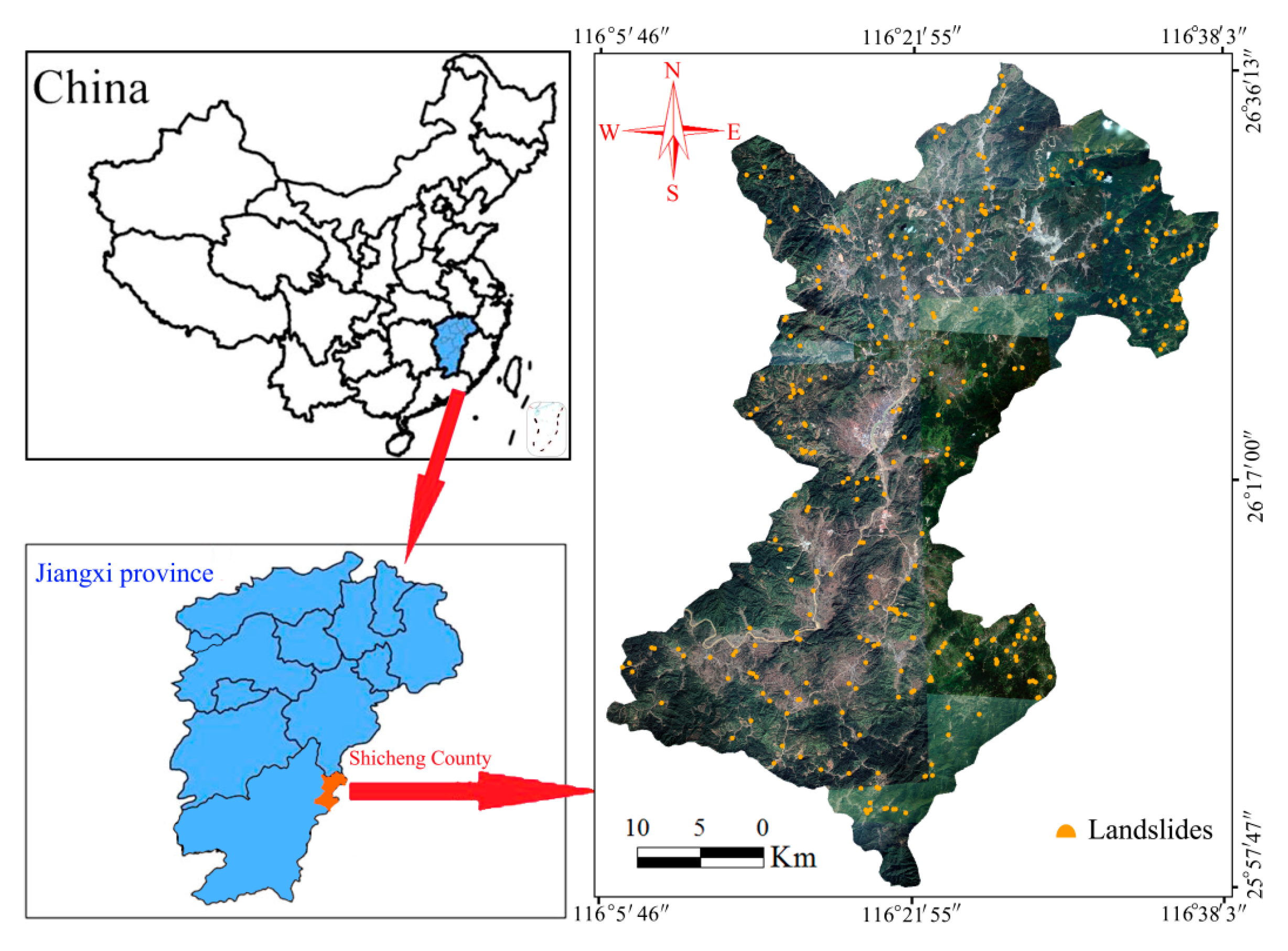
2.1.1. Study Area and Landslide Inventory Information
2.1.2. Landslide-Related Predisposing Factors
- (1)
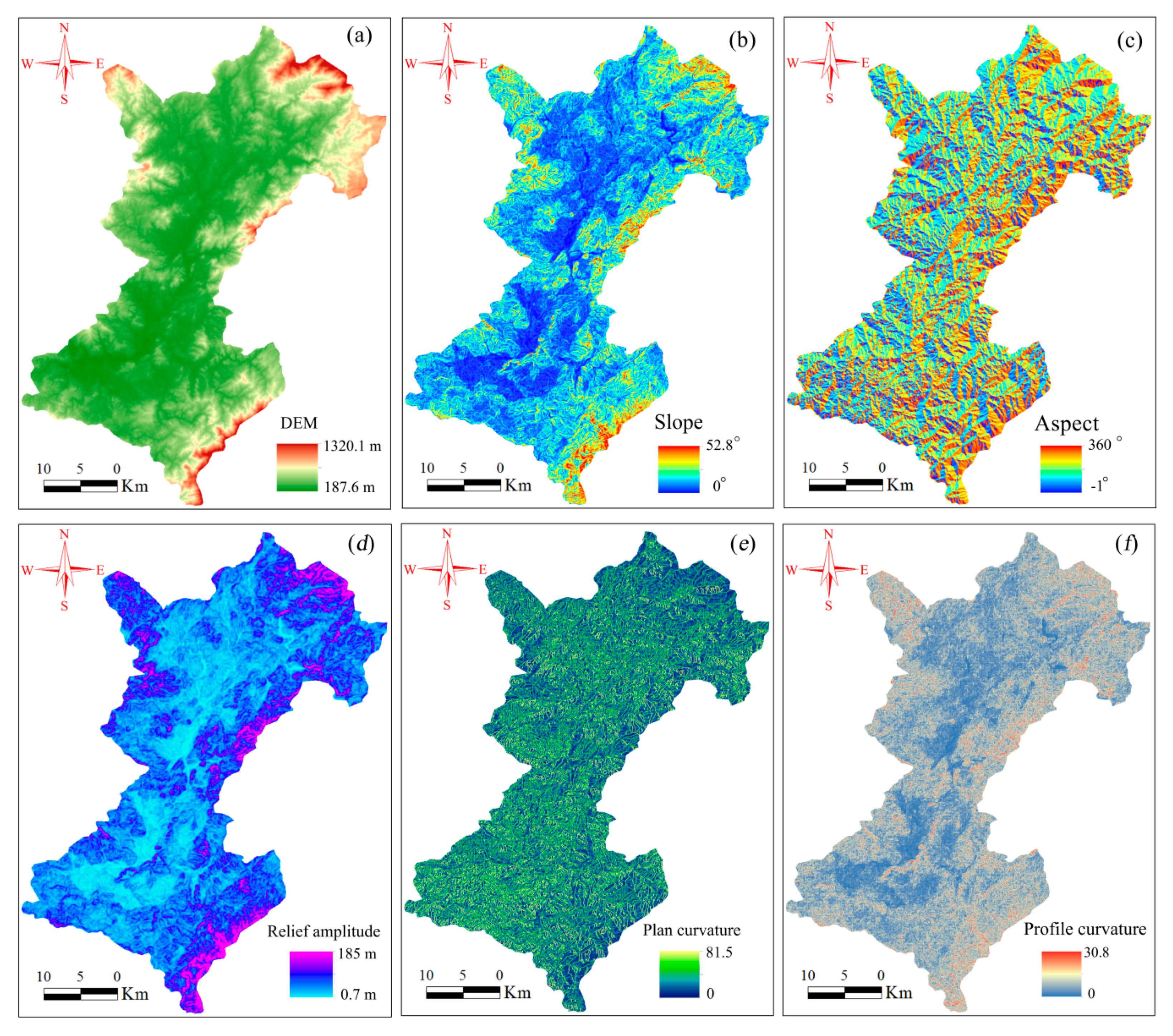
- Topography factors in Shicheng County
- (2)
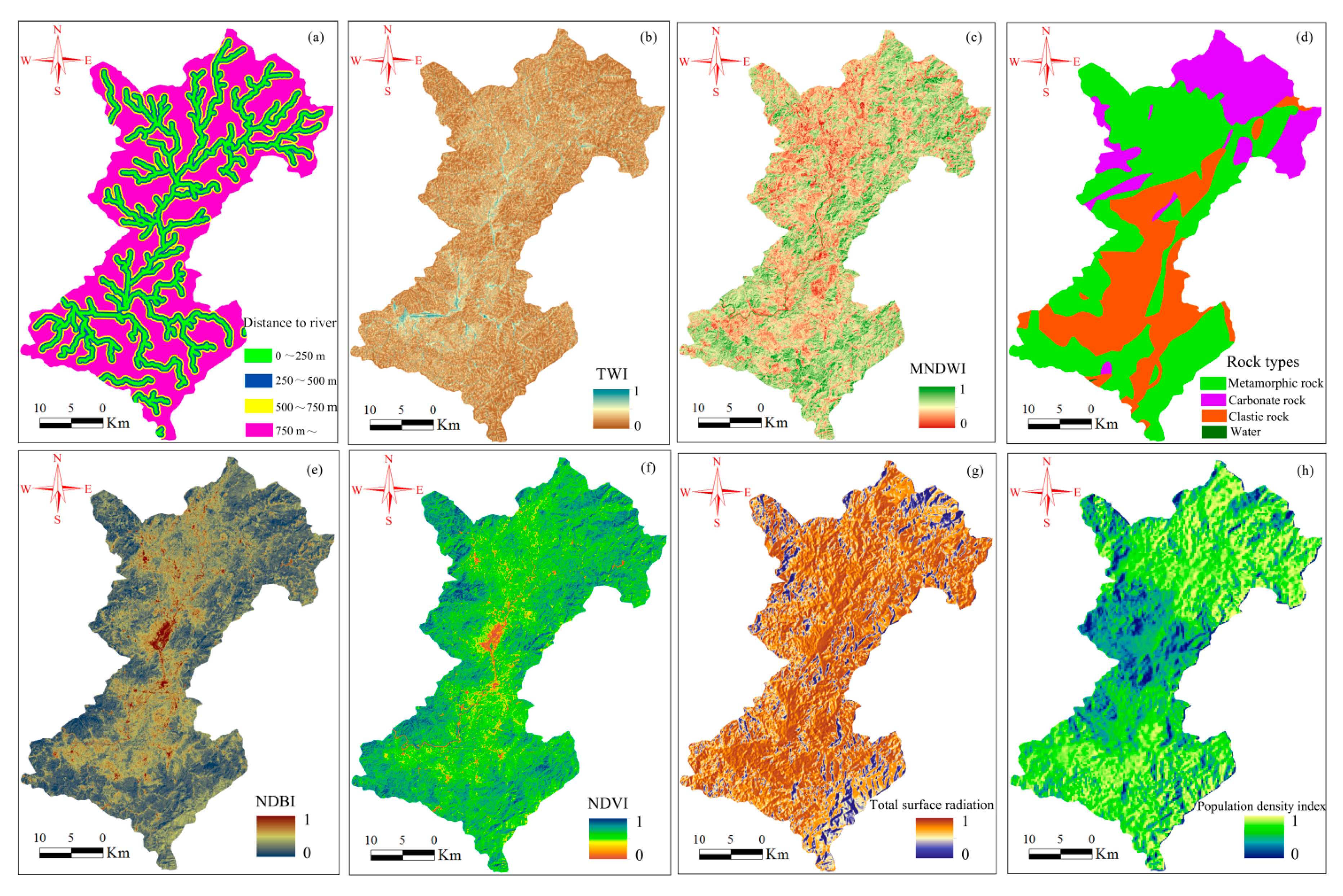
- Hydrological, lithological, and land cover factors
2.1.3. FR and Correlation Analysis of Predisposing Factors
2.2. Methods
2.2.1. Multilayer Perceptron
2.2.2. Theory of PSO-MLP Model
3. Results
3.1. Training and Testing Variables of the Four Models
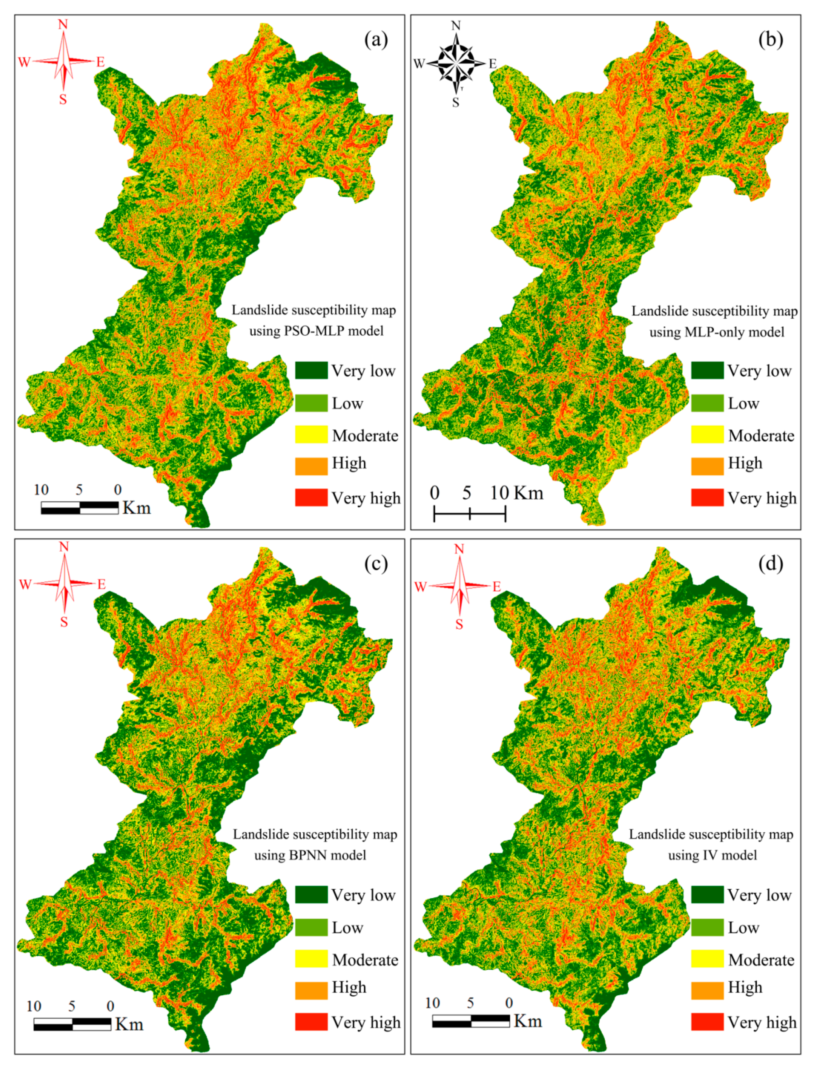
3.2. PSO-MLP Model for LSP
3.3. MLP-Only Model for LSP
3.4. BPNN Model
3.5. IV Model for LSP
4. Discussion
4.1. Frequency Ratio Accuracy Analysis
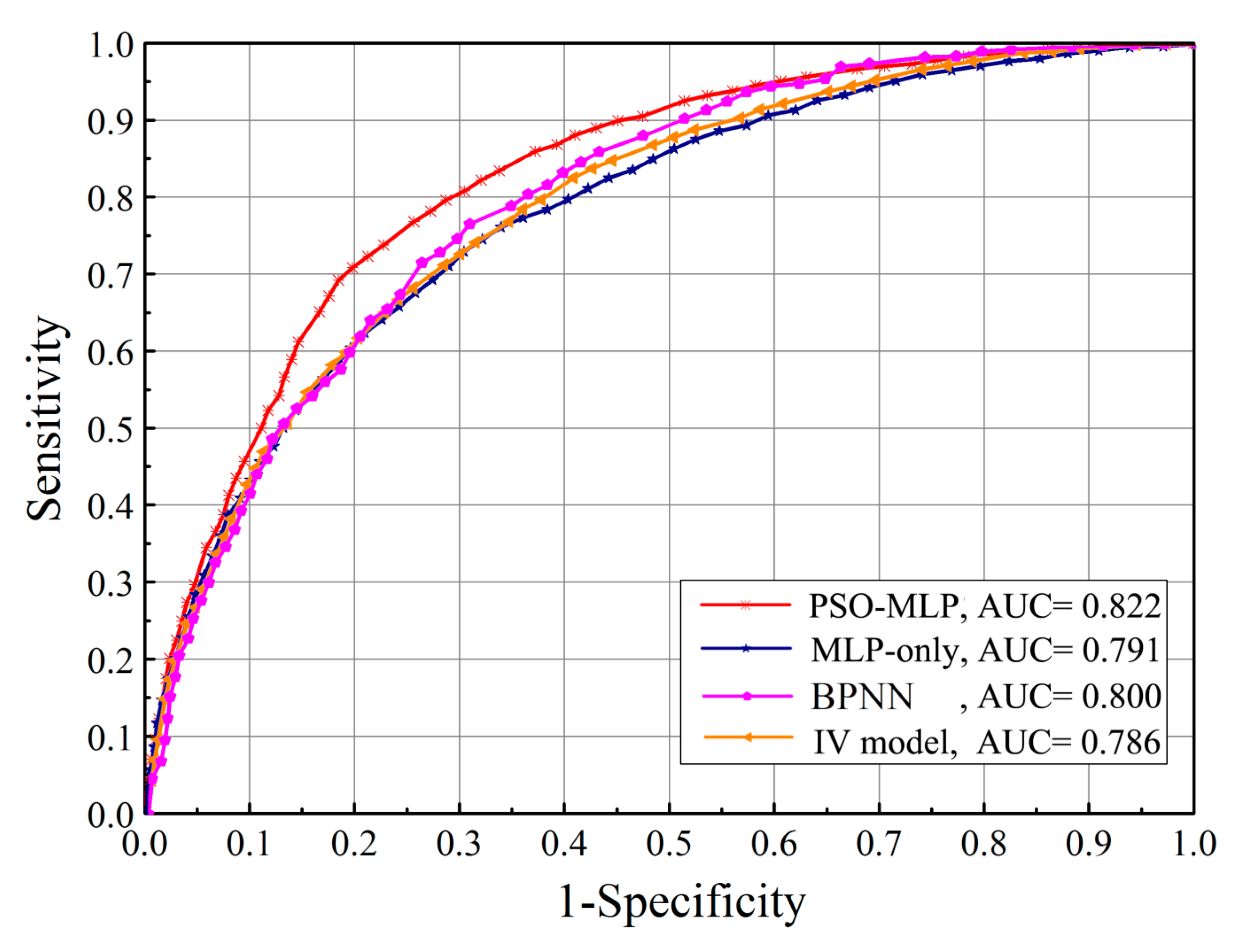
4.2. ROC Accuracies of These Models
4.3. PSO-MLP Model-Building Analysis
5. Conclusions
Author Contributions
Funding
Conflicts of Interest
References
- Assilzadeh, H.; Levy, J.K.; Wang, X. Landslide catastrophes and disaster risk reduction: A GIS framework for landslide prevention and management. Remote Sens. 2010, 2, 2259–2273. [Google Scholar] [CrossRef]
- Huang, F.; Chen, L.; Yin, K.; Huang, J.; Gui, L. Object-oriented change detection and damage assessment using high-resolution remote sensing images, Tangjiao Landslide, Three Gorges Reservoir, China. Environ. Earth Sci. 2018, 77, 183. [Google Scholar] [CrossRef]
- Guo, Z.; Yin, K.; Gui, L.; Liu, Q.; Huang, F.; Wang, T. Regional rainfall warning system for landslides with creep deformation in three gorges using a statistical black box model. Sci. Rep. 2019, 9, 8962. [Google Scholar] [CrossRef] [PubMed]
- Nguyen, P.T.; Tuyen, T.T.; Shirzadi, A.; Pham, B.T.; Shahabi, H.; Omidvar, E.; Amini, A.; Entezami, H.; Prakash, I.; Phong, T.V.; et al. Development of a novel hybrid intelligence approach for landslide spatial prediction. Appl. Sci. 2019, 9, 2824. [Google Scholar] [CrossRef]
- Chen, T.; Niu, R.; Jia, X. A comparison of information value and logistic regression models in landslide susceptibility mapping by using GIS. Environ. Earth Sci. 2016, 75, 867. [Google Scholar] [CrossRef]
- Park, N.W.; Chi, K.H. Quantitative assessment of landslide susceptibility using high-resolution remote sensing data and a generalized additive model. Int. J. Remote Sens. 2008, 29, 247–264. [Google Scholar] [CrossRef]
- Chen, W.; Shahabi, H.; Zhang, S.; Khosravi, K.; Shirzadi, A.; Chapi, K.; Pham, B.T.; Zhang, T.; Zhang, L.; Chai, H.; et al. Landslide susceptibility modeling based on GIS and novel bagging-based kernel logistic regression. Appl. Sci. 2018, 8, 2540. [Google Scholar] [CrossRef]
- Pourghasemi, H.R.; Beheshtirad, M.; Pradhan, B. A comparative assessment of prediction capabilities of modified analytical hierarchy process (M-AHP) and Mamdani fuzzy logic models using Netcad-GIS for forest fire susceptibility mapping. Geomat. Nat. Hazards Risk 2016, 7, 861–885. [Google Scholar] [CrossRef]
- Althuwaynee, O.F.; Pradhan, B.; Park, H.-J.; Lee, J.H. A novel ensemble bivariate statistical evidential belief function with knowledge-based analytical hierarchy process and multivariate statistical logistic regression for landslide susceptibility mapping. Catena 2014, 114, 21–36. [Google Scholar] [CrossRef]
- Nguyen, T.T.N.; Liu, C.-C. A new approach using ahp to generate landslide susceptibility maps in the chen-yu-lan watershed, taiwan. Sensors 2019, 19, 505. [Google Scholar] [CrossRef]
- Hong, H.; Ilia, I.; Tsangaratos, P.; Chen, W.; Xu, C. A hybrid fuzzy weight of evidence method in landslide susceptibility analysis on the Wuyuan area, China. Geomorphology 2017, 290, 1–16. [Google Scholar] [CrossRef]
- Wang, Q.; Wang, Y.; Niu, R.; Peng, L. Integration of information theory, K-means cluster analysis and the logistic regression model for landslide susceptibility mapping in the Three Gorges Area, China. Remote Sens. 2017, 9, 938. [Google Scholar] [CrossRef]
- Huang, F.; Yao, C.; Liu, W.; Li, Y.; Liu, X. Landslide susceptibility assessment in the Nantian area of china: A comparison of frequency ratio model and support vector machine. Geomat. Nat. Hazards Risk 2018, 9, 919–938. [Google Scholar] [CrossRef]
- Pradhan, B.; Lee, S. Landslide susceptibility assessment and factor effect analysis: Backpropagation artificial neural networks and their comparison with frequency ratio and bivariate logistic regression modelling. Environ. Model. Softw. 2010, 25, 747–759. [Google Scholar] [CrossRef]
- Djeddaoui, F.; Chadli, M.; Gloaguen, R. Desertification susceptibility mapping using logistic regression analysis in the Djelfa Area, Algeria. Remote Sens. 2017, 9, 1031. [Google Scholar] [CrossRef]
- Long, N.T.; De Smedt, F. Analysis and mapping of rainfall-induced landslide susceptibility in a Luoi District, Thua Thien Hue province, Vietnam. Water 2018, 11, 51. [Google Scholar] [CrossRef]
- Truong, X.L.; Mitamura, M.; Kono, Y.; Raghavan, V.; Yonezawa, G.; Truong, X.Q.; Do, T.H.; Tien Bui, D.; Lee, S. Enhancing prediction performance of landslide susceptibility model using hybrid machine learning approach of bagging ensemble and logistic model tree. Appl. Sci. 2018, 8, 1046. [Google Scholar] [CrossRef]
- Park, S.; Kim, J. Landslide susceptibility mapping based on random forest and boosted regression tree models, and a comparison of their performance. Appl. Sci. 2019, 9, 942. [Google Scholar] [CrossRef]
- Park, S.-J.; Lee, C.-W.; Lee, S.; Lee, M.-J. Landslide susceptibility mapping and comparison using decision tree models: A case study of Jumunjin Area, Korea. Remote Sens. 2018, 10, 1545. [Google Scholar] [CrossRef]
- Oh, H.-J.; Lee, S. Shallow landslide susceptibility modeling using the data mining models artificial neural network and boosted tree. Appl. Sci. 2017, 7, 1000. [Google Scholar] [CrossRef]
- Nsengiyumva, J.B.; Luo, G.; Nahayo, L.; Huang, X.; Cai, P. Landslide susceptibility assessment using spatial multi-criteria evaluation model in Rwanda. Int. J. Environ. Res. Public Health 2018, 15, 243. [Google Scholar] [CrossRef] [PubMed]
- Xiao, L.; Zhang, Y.; Peng, G. Landslide susceptibility assessment using integrated deep learning algorithm along the China-Nepal Highway. Sensors 2018, 18, 4436. [Google Scholar] [CrossRef] [PubMed]
- Huang, F.; Zhang, J.; Zhou, C.; Wang, Y.; Huang, J.; Zhu, L. A deep learning algorithm using a fully connected sparse autoencoder neural network for landslide susceptibility prediction. Landslides 2019. [Google Scholar] [CrossRef]
- Huang, F.; Yin, K.; Zhang, G.; Gui, L.; Yang, B.; Liu, L. Landslide displacement prediction using discrete wavelet transform and extreme learning machine based on chaos theory. Environ. Earth Sci. 2016, 75, 1376. [Google Scholar] [CrossRef]
- Shao, X.; Ma, S.; Xu, C.; Zhang, P.; Wen, B.; Tian, Y.; Zhou, Q.; Cui, Y. Planet image-based inventorying and machine learning-based susceptibility mapping for the landslides triggered by the 2018 Mw6.6 Tomakomai, Japan Earthquake. Remote Sens. 2019, 11, 978. [Google Scholar] [CrossRef]
- Tien Bui, D.; Shahabi, H.; Shirzadi, A.; Chapi, K.; Alizadeh, M.; Chen, W.; Mohammadi, A.; Ahmad, B.B.; Panahi, M.; Hong, H.; et al. Landslide detection and susceptibility mapping by airsar data using support vector machine and index of entropy models in Cameron Highlands, Malaysia. Remote Sens. 2018, 10, 1527. [Google Scholar] [CrossRef]
- Huang, F.; Yin, K.; He, T.; Zhou, C.; Zhang, J. Influencing factor analysis and displacement prediction in reservoir landslides—A case study of Three Gorges Reservoir (China). Teh. Vjesn. 2016, 23, 617–626. [Google Scholar]
- Bui, D.T.; Pradhan, B.; Lofman, O.; Revhaug, I.; Dick, O.B. Landslide susceptibility mapping at Hoa Binh province (Vietnam) using an adaptive neuro-fuzzy inference system and GIS. Comput. Geosci. 2012, 45, 199–211. [Google Scholar]
- Tien Bui, D.; Shahabi, H.; Shirzadi, A.; Chapi, K.; Hoang, N.-D.; Pham, B.T.; Bui, Q.-T.; Tran, C.-T.; Panahi, M.; Bin Ahmad, B.; et al. A novel integrated approach of relevance vector machine optimized by imperialist competitive algorithm for spatial modeling of shallow landslides. Remote Sens. 2018, 10, 1538. [Google Scholar] [CrossRef]
- Nourani, V.; Pradhan, B.; Ghaffari, H.; Sharifi, S.S. Landslide susceptibility mapping at zonouz plain, iran using genetic programming and comparison with frequency ratio, logistic regression, and artificial neural network models. Nat. Hazards 2014, 71, 523–547. [Google Scholar] [CrossRef]
- Wang, P.; Bai, X.; Wu, X.; Yu, H.; Hao, Y.; Hu, B.X. GIS-based random forest weight for rainfall-induced landslide susceptibility assessment at a humid region in Southern China. Water 2018, 10, 1019. [Google Scholar] [CrossRef]
- Esteves, J.T.; Rolim, G.D.S.; Ferraudo, A.S. Rainfall prediction methodology with binary multilayer perceptron neural networks. Clim. Dyn. 2019, 52, 2319–2331. [Google Scholar] [CrossRef]
- Pham, B.T.; Bui, D.T.; Prakash, I.; Dholakia, M.B. Hybrid integration of multilayer perceptron neural networks and machine learning ensembles for landslide susceptibility assessment at Himalayan Area (India) using GIS. Catena 2017, 149, 52–63. [Google Scholar] [CrossRef]
- Wang, Z.; Zhuowei, H.U.; Zhao, W.; Guo, Q.; Wan, S. Research on regional landslide susceptibility assessment based on multiple layer perceptron—Taking the hilly area in Sichuan as example. J. Disaster Prev. Mitig. Eng. 2015, 35, 691–698. (in Chinese). [Google Scholar]
- Zare, M.; Pourghasemi, H.R.; Vafakhah, M.; Pradhan, B. Landslide susceptibility mapping at VAZ Watershed (Iran) using an artificial neural network model: A comparison between multilayer perceptron (MLP) and radial basic function (RBF) algorithms. Arab. J. Geosci. 2013, 6, 2873–2888. [Google Scholar] [CrossRef]
- Wang, J.; Chang, Q.; Chang, Q.; Liu, Y.; Pal, N.R. Weight noise injection-based MLPS with group lasso penalty: Asymptotic convergence and application to node pruning. IEEE Trans. Cybern. 2018, 1–19. [Google Scholar] [CrossRef]
- Shan, S.L.; Khalil-Hani, M.; Bakhteri, R. An optimized second order stochastic learning algorithm for neural network training. Neurocomputing 2016, 186, 74–89. [Google Scholar]
- Hordri, N.F.; Yuhaniz, S.S.; Shamsuddin, S.M.; Ali, A. Hybrid biogeography based optimization—multilayer perceptron for application in intelligent medical diagnosis. J. Comput. Theor. Nanosci. 2017, 23, 5304–5308. [Google Scholar] [CrossRef]
- Rivera, E.C.; Da, C.A.; Maciel, M.R.; Maciel, F.R. Ethyl alcohol production optimization by coupling genetic algorithm and multilayer perceptron neural network. Appl. Biochem. Biotechnol. 2006, 132, 969–984. [Google Scholar] [CrossRef]
- Yang, Z.; Cheng, W.; Yu, Z.; Jonathan, L. Mini-batch algorithms with Barzilai-Borwein update step. Neurocomputing 2018, 314, 177–185. [Google Scholar] [CrossRef]
- Babanouri, N.; Nasab, S.K.; Sarafrazi, S. A hybrid particle swarm optimization and multi-layer perceptron;algorithm for bivariate fractal analysis of rock fractures roughness. Int. J. Rock Mech. Min. Sci. 2013, 60, 66–74. [Google Scholar] [CrossRef]
- Hungr, O.; Leroueil, S.; Picarelli, L. The Varnes classification of landslide types, an update. Landslides 2014, 11, 167–194. [Google Scholar] [CrossRef]
- Chen, W.; Peng, J.; Hong, H.; Shahabi, H.; Pradhan, B.; Liu, J.; Zhu, A.X.; Pei, X.; Duan, Z. Landslide susceptibility modelling using GIS-based machine learning techniques for Chongren County, Jiangxi province, China. Sci. Total Environ. 2018, 626, 230. [Google Scholar] [CrossRef] [PubMed]
- Hong, H.; Naghibi, S.A.; Pourghasemi, H.R.; Pradhan, B. GIS-based landslide spatial modeling in Ganzhou City, China. Arab. J. Geosci. 2016, 9, 112. [Google Scholar] [CrossRef]
- Marjanović, M.; Kovačević, M.; Bajat, B.; Voženílek, V. Landslide susceptibility assessment using SVM machine learning algorithm. Eng. Geol. 2011, 123, 225–234. [Google Scholar] [CrossRef]
- Nandi, A.; Shakoor, A. A GIS-based landslide susceptibility evaluation using bivariate and multivariate statistical analyses. Eng. Geol. 2010, 110, 11–20. [Google Scholar] [CrossRef]
- Tsangaratos, P.; Benardos, A. Estimating landslide susceptibility through a artificial neural network classifier. Nat. Hazards 2014, 74, 1489–1516. [Google Scholar] [CrossRef]
- Bui, D.T.; Pradhan, B.; Lofman, O.; Revhaug, I.; Dick, O.B. Spatial prediction of landslide hazards in Hoa Binh province (Vietnam): A comparative assessment of the efficacy of evidential belief functions and fuzzy logic models. Catena 2012, 96, 28–40. [Google Scholar]
- He, S.; Pan, P.; Dai, L.; Wanga, H. Application of kernel-based fisher discriminant analysis to map landslide susceptibility in the Qinggan River Delta, Three Gorges, China. Geomorphology 2012, 171, 30–41. [Google Scholar] [CrossRef]
- Chen, W.; Pourghasemi, H.R.; Panahi, M.; Kornejady, A.; Wang, J.L.; Xie, X.S.; Cao, S.B. Spatial prediction of landslide susceptibility using an adaptive neuro-fuzzy inference system combined with frequency ratio, generalized additive model, and support vector machine techniques. Geomorphology 2017, 297, 69–85. [Google Scholar] [CrossRef]
- Li, Y.; Huang, J.; Jiang, S.-H.; Huang, F.; Chang, Z. A web-based GPS system for displacement monitoring and failure mechanism analysis of reservoir landslide. Sci. Rep. 2017, 7, 17171. [Google Scholar] [CrossRef]
- Jiang, S.-H.; Huang, J.; Huang, F.; Yang, J.; Yao, C.; Zhou, C.-B. Modelling of spatial variability of soil undrained shear strength by conditional random fields for slope reliability analysis. Appl. Math. Model. 2018, 63, 374–389. [Google Scholar] [CrossRef]
- Liu, W.; Luo, X.; Huang, F.; Fu, M. Uncertainty of the soil–water characteristic curve and its effects on slope seepage and stability analysis under conditions of rainfall using the Markov Chain Monte Carlo Method. Water 2017, 9, 758. [Google Scholar] [CrossRef]
- Dixon, N.; Brook, E. Impact of predicted climate change on landslide reactivation: Case study of Mam Tor, UK. Landslides 2007, 4, 137–147. [Google Scholar] [CrossRef]
- Duc, D.M. Rainfall-triggered large landslides on 15 December 2005 in Van Canh district, Binh Dinh province, Vietnam. Landslides 2013, 10, 219–230. [Google Scholar] [CrossRef]
- Chen, W.; Xie, X.; Wang, J.; Pradhan, B.; Hong, H.; Bui, D.T.; Duan, Z.; Ma, J. A comparative study of logistic model tree, random forest, and classification and regression tree models for spatial prediction of landslide susceptibility. Catena 2017, 151, 147–160. [Google Scholar] [CrossRef] [Green Version]
- Fortin, J.G.; Anctil, F.; Parent, L.E. Comparison of multiple-layer perceptrons and least squares support vector machines for remote-sensed characterization of in-field Lai patterns—A case study with potato. Can. J. Remote Sens. 2014, 40, 75–84. [Google Scholar] [CrossRef]
- Huang, F.; Huang, J.; Jiang, S.; Zhou, C. Landslide displacement prediction based on multivariate chaotic model and extreme learning machine. Eng. Geol. 2017, 218, 173–186. [Google Scholar] [CrossRef]
- Huang, F.; Luo, X.; Liu, W. Stability analysis of hydrodynamic pressure landslides with different permeability coefficients affected by reservoir water level fluctuations and rainstorms. Water 2017, 9, 450. [Google Scholar] [CrossRef]
- Guo, W.; Wei, H.; Zhao, J.; Zhang, K. Theoretical and numerical analysis of learning dynamics near singularity in multilayer perceptrons. Neurocomputing 2015, 151, 390–400. [Google Scholar] [CrossRef]
- Eberhart, R.C.; Kennedy, J. A new optimizer using particle swarm theory. In Proceedings of the Sixth International Symposium on Micro Machine and Human Science, Nagoya, Japan, 4–6 October 1995; pp. 39–43. [Google Scholar] [CrossRef]
- Huang, F.; Huang, J.; Jiang, S.-H.; Zhou, C. Prediction of groundwater levels using evidence of chaos and support vector machine. J. Hydroinf. 2017, 19, 586–606. [Google Scholar] [CrossRef] [Green Version]
- Huang, F.; Yin, K.; Huang, J.; Lei, G.; Peng, W. Landslide susceptibility mapping based on self-organizing-map network and extreme learning machine. Eng. Geol. 2017, 223, 11–22. [Google Scholar] [CrossRef]
- Pradhan, B.; Lee, S. Regional landslide susceptibility analysis using back-propagation neural network model at Cameron Highland, Malaysia. Landslides 2010, 7, 13–30. [Google Scholar] [CrossRef]
- Sharma, L.P.; Patel, N.; Ghose, M.K.; Debnath, P. Development and application of Shannon’s entropy integrated information value model for landslide susceptibility assessment and zonation in Sikkim Himalayas in India. Nat. Hazards 2015, 75, 1555–1576. [Google Scholar] [CrossRef]


| Factors | Data Type | Value | Grids in Domain | Grid Proportion (%) | Landslide Grid Number | Grid Proportion (%) | Frequency Ratio |
|---|---|---|---|---|---|---|---|
| DEM (m) | Continuous | 0–280.9 | 450,325 | 25.6 | 833 | 30.7 | 1.200 |
| 280.9–360.9 | 544,197 | 31.0 | 943 | 34.8 | 1.124 | ||
| 360.9–454.2 | 308,108 | 17.5 | 307 | 11.3 | 0.646 | ||
| 454.2–560.9 | 181,087 | 10.3 | 341 | 12.6 | 1.222 | ||
| 560.9–676.4 | 127,080 | 7.2 | 199 | 7.3 | 1.016 | ||
| 676.4–805.3 | 86,871 | 4.9 | 82 | 3.0 | 0.612 | ||
| 805.3–969.7 | 41,033 | 2.3 | 4 | 0.1 | 0.063 | ||
| 969.7–1320.1 | 18,636 | 1.1 | 0 | 0 | 0 | ||
| Slope (°) | Continuous | 0–3.9 | 348,797 | 19.8 | 184 | 6.8 | 0.342 |
| 3.9–7.5 | 406,976 | 23.2 | 737 | 27.2 | 1.175 | ||
| 7.5–11.2 | 358,445 | 20.4 | 865 | 31.9 | 1.566 | ||
| 11.2–14.9 | 258,803 | 14.7 | 516 | 19.0 | 1.293 | ||
| 14.9–19.1 | 184,620 | 10.5 | 273 | 10.1 | 0.959 | ||
| 19.1–23.8 | 114,448 | 6.5 | 113 | 4.2 | 0.641 | ||
| 23.8–29.8 | 61,718 | 3.5 | 18 | 0.7 | 0.189 | ||
| 29.8–52.8 | 23,530 | 1.3 | 3 | 0.1 | 0.083 | ||
| Aspect | Continuous | –1 | 359 | 0.02 | 0 | 0 | 0 |
| 0–22.5, 337.5–360 | 204,837 | 11.7 | 258 | 9.5 | 0.817 | ||
| 22.5–67.5 | 176,594 | 10.0 | 233 | 8.6 | 0.856 | ||
| 67.5–112.5 | 212,635 | 12.1 | 439 | 16.2 | 1.339 | ||
| 112.5–157.5 | 230,991 | 13.1 | 379 | 14.0 | 1.064 | ||
| 157.5–202.5 | 225,837 | 12.9 | 276 | 10.2 | 0.793 | ||
| 202.5–247.5 | 211,352 | 12.0 | 263 | 9.7 | 0.807 | ||
| 247.5–292.5 | 239,169 | 13.6 | 464 | 17.1 | 1.259 | ||
| Relief amplitude | Continuous | 0–22.4 | 335,770 | 19.1 | 393 | 14.5 | 0.759 |
| 22.4–38.3 | 420,761 | 23.9 | 924 | 34.1 | 1.425 | ||
| 38. 3–54.2 | 349,311 | 19.9 | 673 | 24.8 | 1.250 | ||
| 54.2–71.5 | 270,334 | 15.4 | 457 | 16.9 | 1.097 | ||
| 71.5–91.0 | 182,134 | 10.4 | 188 | 6.9 | 0.670 | ||
| 91.0–114.9 | 111,395 | 6.3 | 73 | 2.7 | 0.425 | ||
| 114.9–146.7 | 60,885 | 3.5 | 1 | 0.04 | 0.011 | ||
| 146.7–185 | 26,747 | 1.5 | 0 | 0 | 0 | ||
| Plan curvature | Continuous | 0–9.909 | 330,252 | 18.8 | 714 | 26.4 | 1.403 |
| 9.909–18.54 | 351,942 | 20.0 | 748 | 27.6 | 1.379 | ||
| 18.54–27.49 | 269,313 | 15.3 | 468 | 17.3 | 1.127 | ||
| 27.49–37.08 | 206,319 | 11.7 | 292 | 10.8 | 0.918 | ||
| 37.08–47.628 | 167,821 | 9.5 | 198 | 7.3 | 0.765 | ||
| 47.628–58.497 | 133,993 | 7.6 | 84 | 3.1 | 0.407 | ||
| 58.497–70.324 | 126,193 | 7.2 | 74 | 2.7 | 0.380 | ||
| 70.324–81.5 | 171,504 | 9.8 | 131 | 4.8 | 0.496 | ||
| Profile curvature | Continuous | 0–1.694 | 475,975 | 27.1 | 716 | 26.4 | 0.976 |
| 1.694–3.267 | 455,721 | .25.9 | 799 | 29.5 | 1.137 | ||
| 3.267–4.961 | 349,124 | 19.9 | 508 | 18.8 | 0.944 | ||
| 4.961–6.776 | 225,132 | 12.8 | 347 | 12.8 | 0.999 | ||
| 6.776–8.832 | 135,555 | 7.7 | 185 | 6.8 | 0.885 | ||
| 8.832–11.373 | 73,762 | 4.2 | 104 | 3.8 | 0.915 | ||
| 11.373–15.003 | 33,044 | 1.9 | 45 | 1.7 | 0.883 | ||
| 15.003–30.8 | 9024 | 0.5 | 5 | 0.2 | 0.359 | ||
| Distance to river (m) | Discrete | 0–250 | 319,909 | 18.2 | 1237 | 45.7 | 2.508 |
| 250–500 | 291,189 | 16.6 | 447 | 16.5 | 0.996 | ||
| 500–750 | 262,670 | 14.9 | 234 | 8.6 | 0.578 | ||
| 750–3000 | 883,569 | 50.3 | 791 | 29.2 | 0.581 | ||
| TWI | Continuous | 0–6.165 | 327,344 | 18.6 | 430 | 15.9 | 0.852 |
| 6.165–7.256 | 488,501 | 27.8 | 800 | 29.5 | 1.062 | ||
| 7.256–8.346 | 401,144 | 22.8 | 718 | 26.5 | 1.161 | ||
| 8.346–9.601 | 259,094 | .14.7 | 476 | 17.6 | 1.192 | ||
| 9.601–11.128 | 138,598 | 7.9 | 164 | 6.1 | 0.768 | ||
| 11.128–13.037 | 78,193 | 4.4 | 60 | 2.2 | 0.498 | ||
| 13.037–15.6 | 42,782 | 2.4 | 42 | 1.6 | 0.637 | ||
| 15.6–18 | 21,681 | 1.2 | 19 | 0.7 | 0.569 | ||
| MNDWI | Continuous | 0–0.145 | 94,750 | 5.4 | 121 | 4.5 | 0.828 |
| 0.145–0.278 | 187,275 | 10.7 | 324 | 12.0 | 1.122 | ||
| 0.278–0.392 | 258,082 | 14.7 | 492 | 18.2 | 1.237 | ||
| 0.392–0.502 | 296,664 | 16.9 | 616 | 22.7 | 1.347 | ||
| 0.502–0.612 | 297,008 | 16.9 | 541 | 20.0 | 1.182 | ||
| 0.612–0.729 | 273,311 | 15.5 | 348 | 12.8 | 0.826 | ||
| 0.729–0.859 | 211,515 | 12.0 | 183 | 6.8 | 0.561 | ||
| 0.859–1 | 138,732 | 07.9 | 84 | 3.1 | 0.393 | ||
| Rock types | Discrete | Metamorphic rock | 919,176 | 52.3 | 1450 | 53.5 | 1.023 |
| Carbonate rock | 500,159 | 28.5 | 639 | 23.6 | 0.829 | ||
| Clastic rock | 337,500 | 19.2 | 620 | 22.9 | 1.192 | ||
| Water | 502 | 0.03 | 0 | 0 | 0 | ||
| NDBI | Continuous | 0–0.231 | 220,622 | 12.6 | 143 | 5.3 | 0.421 |
| 0.231–0.302 | 407,692 | 23.2 | 324 | 12.0 | 0.516 | ||
| 0.302–0.373 | 385,678 | 21.9 | 502 | 18.5 | 0.844 | ||
| 0.373–0.451 | 283,274 | 16.1 | 575 | 21.2 | 1.317 | ||
| 0.451–0.545 | 211,706 | 12.0 | 561 | 20.7 | 1.719 | ||
| 0.545–0.659 | 142,090 | 8.1 | 349 | 12.9 | 1.593 | ||
| 0.659–0.812 | 77,712 | 4.4 | 200 | 7.4 | 1.670 | ||
| 0.812–1 | 28,563 | 1.6 | 55 | 2.0 | 1.249 | ||
| NDVI | Continuous | 0–0.205 | 21,416 | 1.2 | 18 | 0.7 | 0.545 |
| 0.205–0.363 | 48,274 | 2.7 | 133 | 4.9 | 1.787 | ||
| 0.363–0.46 | 140,192 | 8.0 | 353 | 13.0 | 1.633 | ||
| 0.46–0.53 | 277,504 | 15.8 | 584 | 21.6 | 1.365 | ||
| 0.53–0.593 | 412,360 | 23.5 | 663 | 24.5 | 1.043 | ||
| 0.593–0.651 | 382,238 | 21.8 | 460 | 17.0 | 0.781 | ||
| 0.651–0.721 | 322,632 | 18.4 | 384 | 14.2 | 0.772 | ||
| 0.721–1 | 152,721 | 8.7 | 114 | 4.2 | 0.484 | ||
| Total surface radiation | Continuous | 0–0.459 | 10,052 | 0.6 | 10 | 0.4 | 0.645 |
| 0.459–0.592 | 27,582 | 1.6 | 56 | 2.1 | 1.317 | ||
| 0.592–0.678 | 61,099 | 3.5 | 80 | 3.0 | 0.849 | ||
| 0.678–0.753 | 111,044 | 6.3 | 172 | 6.3 | 1.005 | ||
| 0.753–0.816 | 170,418 | 9.7 | 297 | 11.0 | 1.131 | ||
| 0.816–0.875 | 262,906 | 15.0 | 400 | 14.8 | 0.987 | ||
| 0.875–0.929 | 409,406 | 23.3 | 550 | 20.3 | 0.872 | ||
| 0.929–1 | 704,830 | 40.1 | 1144 | 42.2 | 1.053 | ||
| Population density index | Continuous | 0–0.678 | 20,286 | 1.2 | 7 | 0.3 | 0.224 |
| 0.678–0.733 | 78,566 | 4.5 | 80 | 3.0 | 0.661 | ||
| 0.733–0.776 | 116,553 | 6.6 | 102 | 3.8 | 0.568 | ||
| 0.776–0.820 | 200,139 | 11.4 | 266 | 9.8 | 0.862 | ||
| 0.820–0.863 | 257,308 | 14.6 | 300 | 11.1 | 0.756 | ||
| 0.863–0.906 | 311,063 | 17.7 | 543 | 20.0 | 1.132 | ||
| 0.906–0.949 | 380,425 | 21.6 | 657 | 24.3 | 1.120 | ||
| 0.949–1 | 392,997 | 22.4 | 754 | 27.8 | 1.245 |
| Models | Class | Total Grid Number | Proportion (%) | Landslide Grid Number | Proportion (%) | FR Values |
|---|---|---|---|---|---|---|
| PSO-MLP | Very low | 414,852 | 23.6 | 36 | 1.3 | 0.056 |
| Low | 435,746 | 24.8 | 209 | 7.7 | 0.311 | |
| Moderate | 451,412 | 25.7 | 477 | 17.6 | 0.685 | |
| High | 275,386 | 15.7 | 726 | 26.8 | 1.710 | |
| Very high | 179,941 | 10.2 | 1261 | 46.5 | 4.546 | |
| MLP-only | Very low | 485,954 | 27.7 | 107 | 3.9 | 0.143 |
| Low | 402,491 | 22.9 | 224 | 8.3 | 0.361 | |
| Moderate | 398,323 | 22.7 | 452 | 16.7 | 0.736 | |
| High | 296,913 | 16.9 | 763 | 28.2 | 1.667 | |
| Very high | 173,656 | 9.9 | 1163 | 42.9 | 4.344 | |
| BPNN | Very low | 451,506 | 25.7 | 72 | 2.7 | 0.103 |
| Low | 393,108 | 22.4 | 198 | 7.3 | 0.327 | |
| Moderate | 437,828 | 24.9 | 467 | 17.2 | 0.692 | |
| High | 282,685 | 16.1 | 719 | 26.5 | 1.650 | |
| Very high | 192,208 | 10.9 | 1253 | 46.3 | 4.229 | |
| IV | Very low | 417,155 | 23.7 | 81 | 3.0 | 0.126 |
| Low | 400,663 | 22.8 | 222 | 8.2 | 0.359 | |
| Moderate | 468,615 | 26.7 | 549 | 20.3 | 0.760 | |
| High | 302,688 | 17.2 | 772 | 28.5 | 1.655 | |
| Very high | 168,214 | 9.6 | 1085 | 40.1 | 4.184 |
© 2019 by the authors. Licensee MDPI, Basel, Switzerland. This article is an open access article distributed under the terms and conditions of the Creative Commons Attribution (CC BY) license (http://creativecommons.org/licenses/by/4.0/).
Share and Cite
Li, D.; Huang, F.; Yan, L.; Cao, Z.; Chen, J.; Ye, Z. Landslide Susceptibility Prediction Using Particle-Swarm-Optimized Multilayer Perceptron: Comparisons with Multilayer-Perceptron-Only, BP Neural Network, and Information Value Models. Appl. Sci. 2019, 9, 3664. https://0-doi-org.brum.beds.ac.uk/10.3390/app9183664
Li D, Huang F, Yan L, Cao Z, Chen J, Ye Z. Landslide Susceptibility Prediction Using Particle-Swarm-Optimized Multilayer Perceptron: Comparisons with Multilayer-Perceptron-Only, BP Neural Network, and Information Value Models. Applied Sciences. 2019; 9(18):3664. https://0-doi-org.brum.beds.ac.uk/10.3390/app9183664
Chicago/Turabian StyleLi, Deying, Faming Huang, Liangxuan Yan, Zhongshan Cao, Jiawu Chen, and Zhou Ye. 2019. "Landslide Susceptibility Prediction Using Particle-Swarm-Optimized Multilayer Perceptron: Comparisons with Multilayer-Perceptron-Only, BP Neural Network, and Information Value Models" Applied Sciences 9, no. 18: 3664. https://0-doi-org.brum.beds.ac.uk/10.3390/app9183664