Quadcopter Adaptive Trajectory Tracking Control: A New Approach via Backstepping Technique

Abstract

Nowadays, quadcopter unmanned aerial vehicles play important roles in several real-world applications and the improvement of their control performance has become an increasingly attractive topic of a great number of studies. In this paper, we present a new approach for the design and stability analysis of a quadcopter adaptive trajectory tracking control. Based on the quadcopter nonlinear dynamics model which is obtained by using the Euler–Lagrange approach, the tracking controller is devised via the backstepping control technique. Besides, an adaptive law is proposed to deal with the system parameterized uncertainties and to guarantee that the control input is finite. In addition, the vehicle’s vertical descending acceleration is ensured to not exceed the gravitational acceleration by making use of a barrier Lyapunov function. It is shown that the suitable parameter estimator is stable and the tracking errors are guaranteed to be asymptotically stable simultaneously. By prescribing certain flight conditions, we use numerical simulations to compare the control performance of our method to that of existing approaches. The simulation results demonstrate the effectiveness of the proposed algorithm.

1. Introduction

Unmanned vehicles have currently been playing a crucial role in many aspects of our daily lives where many robots can be used to operate and assist with complex tasks. Especially, unmanned aerial vehicles (UAVs) have been widely researched to create many versatile applications for replacing human from impossible missions and dangerous tasks [1], e.g., in agriculture [2], industry [3,4], and military [5,6]. Quadcopters, which are one of the most popular class of UAVs, have only four actuators, while there are six degrees of freedom, in that it is definitely an under-actuated system. By being able to independently control the speed of each actuator, the vehicle can execute horizontal and vertical movements to carry out a range of different assignments that can range from irrigating large agricultural fields, over investigating and locating lost objects in remote or inaccessible areas (e.g., forests, oceans, deserts), to simulating geographical maps. These tasks are all, somehow, based on a reliable trajectory tracking controller. However, the quadcopter tracking control performance always suffers from several influencing sources such as the system parameterized uncertainties and external disturbances. Therefore, the design and stability analysis of a superior quadcopter trajectory controller becomes one of the most important efforts that scientists and researchers all around the world are undertaking.

1.1. Related Works

It is undeniable that the conventional proportional–integral–derivative (PID) control is still widely used in a variety of many applications all over the world because it is uncomplicated to be applied and acceptably meet given requirements in many studies [7,8,9,10,11,12,13,14,15]. The authors [16,17,18,19] presented the use of a multi-loop control scheme (i.e., inner-loop and outer-loop) to control quadcopters in specific applications. Several authors improved a modified PID approach to design control laws based on nonlinear mathematical models to achieve a position tracking [20,21]. By making use of the discrete linearisation model of tracking errors, the PID controller combined with least quadratic regulation (LQR) were presented in [22,23] to find a discrete control input. When it comes to tracking control of mechanical systems, sliding mode control (SMC) is often employed to guarantee the stability of the systems. The authors of [24,25] presented SMC laws combined with automatically tuning control coefficients to achieve the partial system stability. Typically, the cascade principle is also applied to design a full control law based on the Lyapunov’s direct method that guarantees the asymptotic stability of each loop [25,26,27,28,29,30,31,32] via the backstepping technique [33]. Model predictive control, which obtains some advantages of optimal control, was employed to carry out not only path-tracking problem, but also state constraints [34,35]. In order to tackle external disturbances, a robust nonlinear ${\mathcal{H}}_{\infty }$ controller [36] was proposed to track the reference trajectory.

One of the obstacles of control design for quadcopter is the presence of system parameterized uncertainties in the mathematical model. The system’s parameters must be updated to adjust its control gains when adding several auxiliary devices or replacing some accessories, leading to inconvenience in practice. Therefore, studies [31,37,38] used SMC in combination with an adaptive law based on certainty equivalence principle [33] or artificial neural networks (ANNs) [39,40,41] to deal with uncertainties such as inertial moments and arm length. By using Fuzzy logic, the authors [42] found a control law without any advance knowledge about mathematical model of quadcopter. When ANNs and Fuzzy logic are applied to identify the system model instead of using the explicit mathematical model, the tracking performance of the considered system has still been controversial topic.

On the other hand, the above existing works still have some negative viewpoints in trajectory tracking problem. Many kinds of PID control (i.e., conventional form, modified form, and combination with LQR) may not clearly show the asymptotic stability. The control schemes based on SMC always use a sign function to switch between two modes, i.e., controlled variables are either outside or within the sliding surface, leading to chattering phenomenon. In other studies [17,25,43], the second order SMC was applied to reduce a chattering phenomenon to enhance the tracking performance. Moreover, it is a considerable drawback that SMC state variables have to reach the sliding surface in finite time to guarantee the convergence at the origin, which was ignored in the above papers. Based on the cascade principle, only a linear system which is a result of combining all linear stable subsystems can directly achieve stability. In contrast, a nonlinear model systems may not be stable because of the appearance of a finite escape time phenomenon which may cause state variables to become infinity in finite time (Chapter 3 in [44]), leading to a highly undesirable case in automatic control systems.

1.2. Main Contributions

In this study, we design control laws and an adaptive law that guarantee both the system stability and trajectory tracking for quadcopter in the presence of unknown constant parameters such as inertial moment, arm length, and drag coefficients. Firstly, the quadcopter dynamics is parallelly separated into horizontal and vertical dynamics because any motions in three-dimensional space are their linear combination. The tracking ability of the entire horizontal subsystem is guaranteed by using the backstepping technique based on Lyapunov’s direct method [33], while most of the previous above papers [17,24,25,31] typically separated a horizontal subsystem into position and attitude parts and did not carry out a stability analysis of this subsystem as a whole. Additionally, an adaptive law is proposed to deal with system parameterized uncertainties which may be difficult to precisely measured in many practical cases. To clearly demonstrate the effectiveness of the proposed approach, the LaSalle’s theorem is applied to ensure that the parameter estimator is stable and tracking errors are asymptotically stable at the origin. Finally, the motion along the vertical axis is improved by employing the barrier Lyapunov function [45], which allows smooth altitude changes that results in a capability of descent lower than it freely fall to guarantee tracking error to be within the pre-specified bound.

1.3. Organization

The remainder of this paper consists of five parts. In Section 2, we define several symbols and notation used throughout this paper and introduce the mathematical dynamics and all model parameters. Section 3 describes state feedback controls and an adaptive law to prove the tracking asymptotic stability of the entire system. In Section 4, the validity of the proposed method is verified by the comparative performance of our approach and the other existing works. The final section concludes this paper.

2. Preliminaries and Mathematical Model

The following notations and symbols will be used throughout this paper. The notations x or X are the vector and bold letter $\mathbf{X}$ is the matrix. Next, ${\mathbb{R}}^n$ stands for set of real n-dimensional vector, ${\mathbb{R}}^{n\times m}$ denotes set of real n-row and m-column matrix, and ${\mathbf{I}}_n$ is the $n\times n$ identity matrix. $c\varphi =cos\left(\varphi \right)$, $s\varphi =sin\left(\varphi \right)$, $c\theta =cos\left(\theta \right)$, $s\theta =sin\left(\theta \right)$, $c\psi =cos\left(\psi \right)$, and $s\psi =sin\left(\psi \right)$ are denoted. $\mathrm{vec}\left(\mathbf{X}\right)$ denotes a vectorization of a matrix $\mathbf{X}$, e.g., if $\mathbf{X}=\left[X_1,X_2,X_3\right]$ then $\mathrm{vec}\left(\mathbf{X}\right)={\left[X_1^T,X_2^T,X_3^T\right]}^T$. $\mathrm{vec}(\dot{\mathbf{X}})$ represents the first time-derivative of each its elements. Lastly, $\left|•\right|$ and ⊗ are used to represent the absolute and Kronecker product operators, respectively.

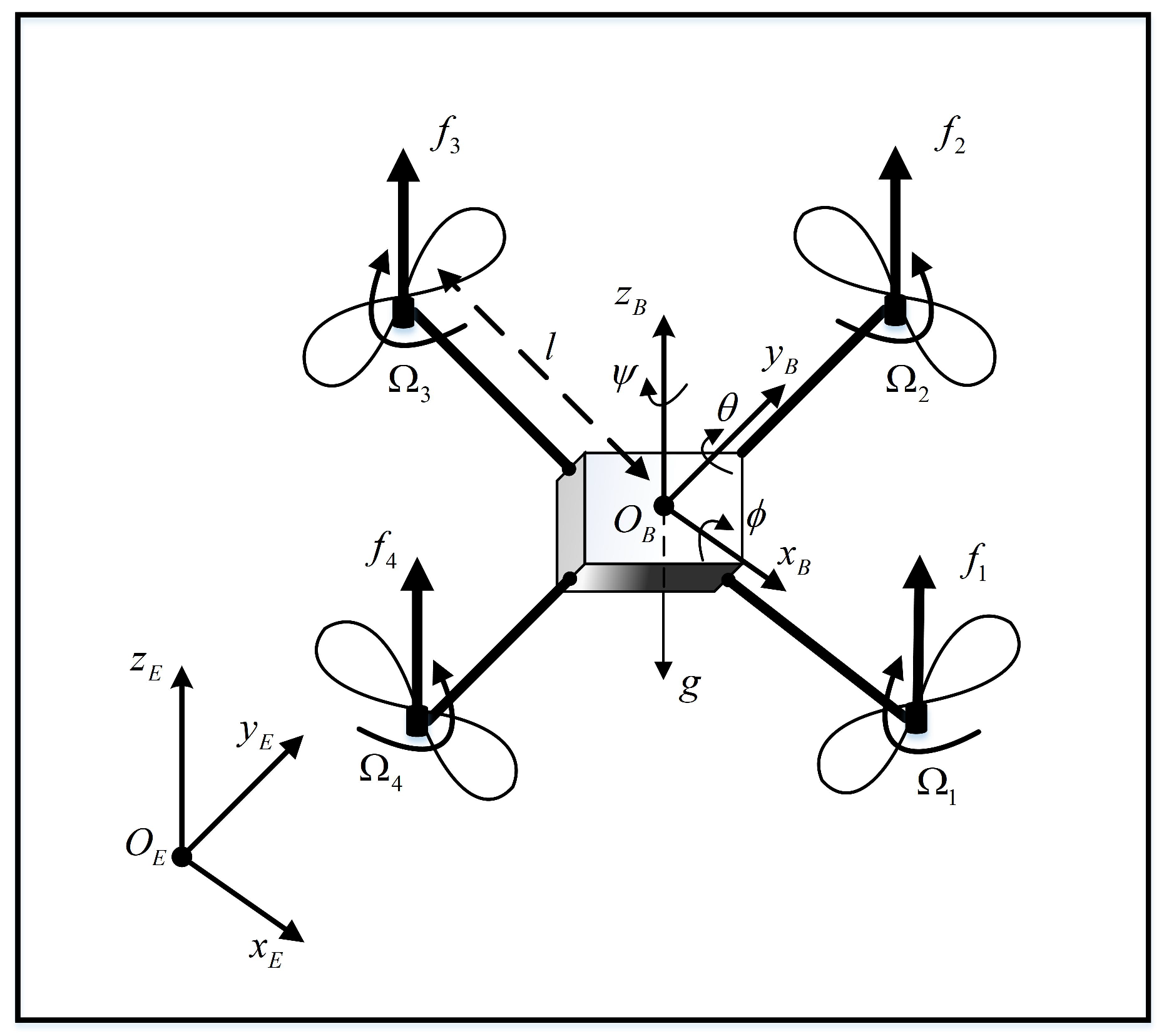
In this section, the model, the parameters, and the variables of Unmanned Arial Vehicles, specifically Plus-Configuration are introduced in Figure 1,

Table 1. The quadcopter parameters.

Definition	Symbol	Unit
Mass of whole UAV	m	kg
Gravitational acceleration	g	m/s${}^2$
Arm length	l	m
Thrust coefficient	b	N·s${}^2$/rad${}^2$
Drag coefficient	d	N·s${}^2$/rad${}^2$
Inertial moment about x-axis	$I_{xx}$	kg·m${}^2$
Inertial moment about y-axis	$I_{yy}$	kg·m${}^2$
Inertial moment about z-axis	$I_{zz}$	kg·m${}^2$
Drag moment coefficient	${\mu }_i$	s${}^{-1}$

and

Table 2. The quadcopter variables.

Definition	Symbol	Unit
Position in Earth frame	$x,y,z$	m
Position in Body frame	$x_B,y_B,z_B$	m
Roll, Pitch, Yaw angles	$\varphi ,\theta ,\psi$	rad
Rotor speed	${\mathsf{\Omega }}_1,{\mathsf{\Omega }}_2,{\mathsf{\Omega }}_3,{\mathsf{\Omega }}_4$	rad/s
Thrust force	$f_1,f_2,f_3,f_4$	N

, respectively. In order to meet the requirements based on path tracking, a control law is expectedly designed to automatically change four different rotor speeds ${\mathsf{\Omega }}_i$. The intermediate control inputs [12] will be shown as follows:

$$\begin{array}{cc}\hfill & U_1=b\left({\mathsf{\Omega }}_1^2+{\mathsf{\Omega }}_2^2+{\mathsf{\Omega }}_3^2+{\mathsf{\Omega }}_4^2\right)\hfill \\ \hfill & U_2=b\left(-{\mathsf{\Omega }}_2^2+{\mathsf{\Omega }}_4^2\right)\hfill \\ \hfill & U_3=b\left({\mathsf{\Omega }}_1^2-{\mathsf{\Omega }}_3^2\right)\hfill \\ \hfill & U_4=d\left(-{\mathsf{\Omega }}_1^2+{\mathsf{\Omega }}_2^2-{\mathsf{\Omega }}_3^2+{\mathsf{\Omega }}_4^2\right)\hfill \end{array}$$

(1)

where $U_1$ impacts on vertical movement, $U_2$ and $U_3$ are able to drive this system move forward, back, turn left and right in the horizontal plane, and $U_4$ makes this system rotate at a standing point.

First, to achieve the mathematical model of the considered quadcopter, we use the Euler–Lagrange approach to describe the system position $\zeta ={\left[x,y,z\right]}^T$ in the Earth-fixed frame. The Euler–Lagrange equations are applied into the system following a translational $E_{trans}$ and a potential energy $E_{pot}$ [12] as follows:

$$\begin{array}{cc}\hfill & \frac{d}{dt}\left[\frac{\partial }{\partial \dot{\zeta }}{L}_{trans}\left(\dot{\zeta },\zeta \right)\right]-\frac{\partial }{\partial \zeta }{L}_{trans}=\mathbf{R}{f}_B\hfill \end{array}$$

(2)

$$\begin{array}{cc}\hfill & L_{trans}\left(\dot{\zeta },\zeta \right)=E_{trans}+E_{pot}\hfill \end{array}$$

(3)

$$\begin{array}{cc}\hfill & E_{trans}=\frac{m}{2}{\dot{\zeta }}^T\dot{\zeta }\hfill \end{array}$$

(4)

$$\begin{array}{cc}\hfill & E_{pot}=-mgz\hfill \end{array}$$

(5)

$$\begin{array}{cc}\hfill & \mathbf{R}=\left[\begin{array}{ccc}c\psi c\theta & c\psi s\theta s\varphi -s\psi c\varphi & c\psi s\theta c\varphi +s\psi s\varphi \\ s\psi c\theta & s\psi s\theta s\varphi +c\psi c\varphi & s\psi s\theta c\varphi -c\psi s\varphi \\ s\theta & c\theta s\varphi & c\theta c\varphi \end{array}\right]\hfill \end{array}$$

(6)

$$\begin{array}{cc}\hfill & f_B={\left[0,0,U_1\right]}^T\hfill \end{array}$$

(7)

where matrix R in (6) is the transformation matrix from body to Earth-fixed frame and control input $f_B$ (7) contains lift force $U_1$ in $z-axis$ of body frame in (1). Substituting (3), (4), (5), (6), and (7) into (2) to obtain the second ordinary differential equations of dynamics in (8):

$$\begin{array}{c}\hfill \frac{d}{dt}\left(\dot{\zeta }\right)=\frac{U_1}{m}\left[\begin{array}{c}\left(c\psi s\theta c\varphi +s\psi s\varphi \right)\\ \left(s\psi s\theta c\varphi -c\psi s\varphi \right)\\ \left(c\theta c\varphi \right)\end{array}\right]+\left[\begin{array}{c}0\\ 0\\ -g\end{array}\right]\end{array}$$

(8)

Considering the dynamic rotation model based on the energy of rotation through Euler–Lagrange method with hovering assumption. The second ordinary differential equations of Roll, Pitch, and Yaw angles will be described with several unknown parameters in Table 1:

$$\begin{array}{cc}\hfill & \ddot{\varphi }=a_1\dot{\theta }\dot{\psi }-{\mu }_1\dot{\varphi }+b_1{U}_2\hfill \\ \hfill & \ddot{\theta }=a_2\dot{\varphi }\dot{\psi }-{\mu }_2\dot{\theta }+b_2{U}_3\hfill \\ \hfill & \ddot{\psi }=a_3\dot{\varphi }\dot{\theta }-{\mu }_3\dot{\psi }+b_3{U}_4\hfill \end{array}$$

(9)

$$\begin{array}{cc}\hfill & a_1=\frac{I_{yy}-I_{zz}}{I_{xx}}{a}_2=\frac{I_{zz}-I_{xx}}{I_{yy}}{a}_3=\frac{I_{xx}-I_{yy}}{I_{zz}}\hfill \\ \hfill & b_1=\frac{l}{I_{xx}}{b}_2=\frac{l}{I_{yy}}{b}_3=\frac{1}{I_{zz}}\hfill \end{array}$$

(10)

Assumption 1.

It is assumed that this considered system does not flip in the air and lift force $U_1$ is positive when the quadcopter is in operation.

$$\begin{array}{c}\hfill \frac{-\pi }{2}<\varphi <\frac{\pi }{2},\frac{-\pi }{2}<\theta <\frac{\pi }{2},U_1>0\end{array}$$

(11)

Assumption 2.

The considered system is required to track a reference trajectory vector ${\left[x_d\left(t\right),y_d\left(t\right),z_d\left(t\right)\right]}^T$ which is differentiable up to four times. Especially, the second derivatives of $z_d\left(t\right)$, in particular, must satisfy the following condition [32] to ensure that a quadcopter is not allowed to land faster than it freely fall under gravity with a strictly positive constant $k_0$:

$$\begin{array}{c}\hfill \inf \left(m{\ddot{z}}_d\left(t\right)+mg\right)\ge k_0\end{array}$$

(12)

Now, the control objective is to design an adaptive backstepping controller to steer the quadcopter to asymptotically track the desired trajectory reference $x_d$, $y_d$, and $z_d$, despite the presence of system model uncertainties. Moreover, the stability of the entire system is analysed and established by using Lyapunov’s direct method when combining suitable parameter estimators and control law based on certainty equivalence principle and backstepping technique [33], respectively.

3. Trajectory Tracking Control: Adaptive Backstepping Design and Stability Analysis

In order to achieve expected performance, the mathematical model (8) can be separated into two subsystems: horizontal (represented by the first two equations) and vertical motions (represented by the last equation).

3.1. Horizontal Position Controller

Considering the desired trajectory is projected in the $xy$-plane. The purpose is that horizontal position $(x,y)$ is able to track this reference asymptotically.

$$\begin{array}{c}\hfill X_d={\left[x_d,y_d\right]}^T\end{array}$$

(13)

The horizontal state variables (14), (15) and virtual control input (16) can be shown as:

$$\begin{array}{cc}\hfill X& ={\left[x,y\right]}^T\hfill \end{array}$$

(14)

$$\begin{array}{cc}\hfill V& ={\left[\dot{x},\dot{y}\right]}^T\hfill \end{array}$$

(15)

$$\begin{array}{cc}\hfill \vartheta & =\left[\begin{array}{c}cos\left(\varphi \right)sin\left(\theta \right)\\ sin\left(\varphi \right)\end{array}\right]\hfill \end{array}$$

(16)

It is easily seen that the two first equations in (8) becomes (17) and (18) by using (14), (15), and (16):

$$\begin{array}{cc}\hfill \dot{X}& =V\hfill \end{array}$$

(17)

$$\begin{array}{cc}\hfill \dot{V}& =\mathbf{A}(U_1,\psi )\vartheta \hfill \end{array}$$

(18)

$$\begin{array}{cc}\hfill \mathbf{A}(U_1,\psi )& =\frac{U_1}{m}\left[\begin{array}{cc}cos\left(\psi \right)& sin\left(\psi \right)\\ sin\left(\psi \right)& -cos\left(\psi \right)\end{array}\right]\hfill \end{array}$$

(19)

By calculating the virtual control (16), this system change its $\theta -Pitch$ or $\varphi -Roll$ angle to move along the $x-axis$ or $y-axis$, respectively. The tracking error is chosen as:

$$\begin{array}{cc}\hfill & \xi =X-X_d\hfill \\ \hfill & \dot{\xi }=V-{\dot{X}}_d\hfill \end{array}$$

(20)

The first Lyapunov candidate function (21) and its time-derivative (22) along the solution of model (20):

$$\begin{array}{cc}\hfill & V_1=\frac{1}{2}{\xi }^T\xi \hfill \end{array}$$

(21)

$$\begin{array}{cc}\hfill & {\dot{V}}_1={\xi }^T\left(V-{\dot{X}}_d\right)\hfill \end{array}$$

(22)

The virtual control input for (22) with positive definite matrix ${\mathbf{K}}_1\in {\mathbb{R}}^{2\times 2}$ can be selected as:

$$\begin{array}{c}\hfill r_1={\dot{X}}_d-{\mathbf{K}}_1\xi \end{array}$$

(23)

The second Lyapunov candidate function (24) and its time-derivative along solution of model (20) and (23):

$$\begin{array}{cc}\hfill V_2=& V_1+\frac{1}{2}{\left(V-r_1\right)}^T\left(V-r_1\right)\hfill \\ \hfill {\dot{V}}_2=& {\xi }^T\left(V-{\dot{X}}_d+r_1-r_1\right)+{\left(V-r_1\right)}^T\left(\mathbf{A}(U_1,\psi )\vartheta -{\dot{r}}_1\right)\hfill \end{array}$$

(24)

$$\begin{array}{cc}\hfill =& -{\xi }^T{\mathbf{K}}_1\xi +{\left(V-r_1\right)}^T\left(\mathbf{A}(U_1,\psi )\vartheta -{\dot{r}}_1+\xi \right)\hfill \end{array}$$

(25)

It can be seen that when the input $U_1$ satisfies Assumption 1, the matrix $\mathbf{A}(U_1,\psi )$ is definitely invertible. The virtual control input for (25) with positive definite matrix ${\mathbf{K}}_2\in {\mathbb{R}}^{2\times 2}$ can be selected as:

$$\begin{array}{c}\hfill r_2=\mathbf{A}{(U_1,\psi )}^{-1}\left[{\dot{r}}_1-\xi -{\mathbf{K}}_2\left(V-r_1\right)\right]\end{array}$$

(26)

The Roll and Pitch dynamic models in (9) are considered to find the control input:

$$\begin{array}{cc}\hfill \dot{\vartheta }& =\mathbf{B}(\varphi ,\theta )\dot{q}\hfill \\ \hfill \mathbf{B}(\varphi ,\theta )& =\left[\begin{array}{cc}-sin\left(\varphi \right)sin\left(\theta \right)& cos\left(\varphi \right)cos\left(\theta \right)\\ cos\left(\varphi \right)& 0\end{array}\right]\hfill \end{array}$$

(27)

$$\begin{array}{cc}\hfill \dot{q}& =\left[\begin{array}{c}\dot{\varphi }\\ \dot{\theta }\end{array}\right]\hfill \end{array}$$

(28)

Remark 1.

Generally, the horizontal movement is divided into position and attitude subsystems with separate control laws. Previous studies presented a stability standard for each subsystem which led to the possibility of the appearance of the finite escape time phenomenon. Equation (27) shows the relationship between the movement in the $xy$-plane and attitude angles to prove the stability of the whole system in Theorem 1, which will definitely eliminate the finite escape time phenomenon.

The third Lyapunov candidate function (29) and its time-derivative along solution of models (20), (23), and (26):

$$\begin{array}{cc}\hfill V_3=& V_2+\frac{1}{2}{\left(\vartheta -r_2\right)}^T\left(\vartheta -r_2\right)\hfill \\ \hfill {\dot{V}}_3=& -{\xi }^T{\mathbf{K}}_1\xi -{\left(V-r_1\right)}^T{\mathbf{K}}_2\left(V-r_1\right)\hfill \end{array}$$

(29)

$$\begin{array}{cc}\hfill & +{\left(\vartheta -r_2\right)}^T\left(\mathbf{B}(\varphi ,\theta )\dot{q}-{\dot{r}}_2+\mathbf{A}{(U_1,\psi )}^T\left(V-r_1\right)\right)\hfill \end{array}$$

(30)

Because the matrix $\mathbf{B}(\varphi ,\theta )$ is invertible, the virtual control input for (30) with positive definite matrix ${\mathbf{K}}_3\in {\mathbb{R}}^{2\times 2}$ can be selected as:

$$\begin{array}{c}\hfill r_3=\mathbf{B}{(\varphi ,\theta )}^{-1}\left[{\dot{r}}_2-\mathbf{A}{(U_1,\psi )}^T\left(V-r_1\right)-{\mathbf{K}}_3\left(\vartheta -r_2\right)\right]\end{array}$$

(31)

In order to obtain the horizontal tracking, two first Euler angle models in (9) are investigated to find the intermediate control input $U={\left[U_2,U_3\right]}^T$.

$$\begin{array}{cc}\hfill & \ddot{q}={\mathbf{E}}^{-1}\left[\mathbf{E}C\left(\dot{\varphi },\dot{\theta },\dot{\psi },{\mu }_4,{\mu }_5\right)+U\right]\hfill \end{array}$$

(32)

$$\begin{array}{cc}\hfill & \mathbf{E}C\left(\dot{\varphi },\dot{\theta },\dot{\psi },{\mu }_4,{\mu }_5\right)={\mathbf{C}}_1\left(\dot{\varphi },\dot{\theta },\dot{\psi }\right)\mathsf{\Gamma }\hfill \end{array}$$

(33)

where

$$\begin{array}{c}\hfill {\mathbf{E}}^{-1}=\left[\begin{array}{cc}{b}_1& 0\\ 0& b_2\end{array}\right],C\left(\dot{\varphi },\dot{\theta },\dot{\psi },{\mu }_4,{\mu }_5\right)=\left[\begin{array}{c}\dot{\theta }\dot{\psi }{a}_1-\dot{\varphi }{\mu }_4\\ \dot{\varphi }\dot{\psi }{a}_3-\dot{\theta }{\mu }_5\end{array}\right]\end{array}$$

(34)

$$\begin{array}{c}\hfill {\mathbf{C}}_1\left(\dot{\varphi },\dot{\theta },\dot{\psi }\right)=\left[\begin{array}{cccc}\dot{\theta }\dot{\psi }& -\dot{\varphi }& 0& 0\\ 0& 0& \dot{\varphi }\dot{\psi }& -\dot{\theta }\end{array}\right],\mathsf{\Gamma }=\left[\begin{array}{c}{a}_1/b_1\\ {\mu }_4/b_1\\ a_3/b_2\\ {\mu }_5/b_2\end{array}\right]\end{array}$$

(35)

Assumption 3.

It is assumed that $\mathit{E},\mathsf{\Gamma }$ are model uncertainties because they absolutely depend on the environment, material, and arrangement of devices in a real model. Additionally, $\mathit{E}$ and Γ satisfy the following boundary conditions:

$$\begin{array}{cc}\hfill & {\mathsf{\Gamma }}_{i-min}\le {\mathsf{\Gamma }}_i\le {\mathsf{\Gamma }}_{i-max}\hfill \end{array}$$

(36)

$$\begin{array}{cc}\hfill & b_{i-min}\le b_i\le b_{i-max}\hfill \end{array}$$

(37)

Remark 2.

It can be seen that the Equation (32) is transformed to separate matched uncertainty Γ and multiplied control input parameter E. This is the proposition to present an adaptive law which can address the aforementioned unknown parameter problem.

The fourth Lyapunov candidate function with positive definite matrices ${\mathbf{Q}}_1={\mathbf{Q}}_1^T$ and ${\mathbf{Q}}_2={\mathbf{Q}}_2^T\in {\mathbb{R}}^{4\times 4}$ is shown in (38), while $\widehat{\mathsf{\Gamma }}$ and $\widehat{\mathbf{E}}$ are the estimated values of $\mathsf{\Gamma }$ and $\mathbf{E}$, respectively:

$$\begin{array}{cc}\hfill V_4=& V_3+\frac{1}{2}{\left(\dot{q}-r_3\right)}^T\mathbf{E}\left(\dot{q}-r_3\right)+\frac{1}{2}{\left(\mathsf{\Gamma }-\widehat{\mathsf{\Gamma }}\right)}^T{\mathbf{Q}}_1^{-1}\left(\mathsf{\Gamma }-\widehat{\mathsf{\Gamma }}\right)+\frac{1}{2}\mathrm{vec}{\left(\mathbf{E}-\widehat{\mathbf{E}}\right)}^T{\mathbf{Q}}_2^{-1}\mathrm{vec}\left(\mathbf{E}-\widehat{\mathbf{E}}\right)\hfill \\ \hfill {\dot{V}}_4=& -{\xi }^T{\mathbf{K}}_1\xi -{\left(V-r_1\right)}^T{\mathbf{K}}_2\left(V-r_1\right)-{\left(\vartheta -r_2\right)}^T{\mathbf{K}}_3\left(\vartheta -r_2\right)\hfill \end{array}$$

(38)

$$\begin{array}{cc}\hfill & +{\left(\dot{q}-r_3\right)}^T\left(\mathbf{E}\ddot{q}-\mathbf{E}{\dot{r}}_3+\mathbf{B}{(\varphi ,\theta )}^T\left(\vartheta -r_2\right)\right)-{\left(\mathsf{\Gamma }-\widehat{\mathsf{\Gamma }}\right)}^T{\mathbf{Q}}_1^{-1}\dot{\widehat{\mathsf{\Gamma }}}-\mathrm{vec}{\left(\mathbf{E}-\widehat{\mathbf{E}}\right)}^T{\mathbf{Q}}_2^{-1}\mathrm{vec}\left(\dot{\widehat{\mathbf{E}}}\right)\hfill \end{array}$$

(39)

The proposed intermediate control law (40) with positive definite matrix ${\mathbf{K}}_4\in {\mathbb{R}}^{2\times 2}$ and the proposed adaptive laws (41) and (42) can be selected as:

$$\begin{array}{cc}\hfill U=& -\mathbf{B}{(\varphi ,\theta )}^T\left(\vartheta -r_2\right)-{\mathbf{K}}_4\left(\dot{q}-r_3\right)-{\mathbf{C}}_1\left(\dot{\varphi },\dot{\theta },\dot{\psi }\right)\widehat{\mathsf{\Gamma }}+\widehat{\mathbf{E}}{\dot{r}}_3\hfill \end{array}$$

(40)

$$\begin{array}{cc}\hfill \dot{\widehat{\mathsf{\Gamma }}}=& -{\mathbf{Q}}_1{\mathbf{C}}_1{\left(\dot{\varphi },\dot{\theta },\dot{\psi }\right)}^T\left(r_3-\dot{q}\right)\hfill \end{array}$$

(41)

$$\begin{array}{cc}\hfill \mathrm{vec}\left(\dot{\widehat{E}}\right)=& -{\mathbf{Q}}_2\left({\dot{r}}_3\otimes \left(\dot{q}-r_3\right)\right)\hfill \end{array}$$

(42)

Theorem 1.

In order to achieve horizontal asymptotic tracking stability, there exist positive control parameters ${\mathit{K}}_1$, ${\mathit{K}}_2$, ${\mathit{K}}_3$, ${\mathit{K}}_4$, ${\mathit{Q}}_1$, and ${\mathit{Q}}_2$ such that the proposed control law (40) and adaptive laws (41), (42) can be applied to the system models (8) and (9) under Assumptions 1 and 3.

Proof of Theorem 1.

By selecting appropriate positive constant matrices ${\mathbf{K}}_1$, ${\mathbf{K}}_2$, ${\mathbf{K}}_3$, ${\mathbf{K}}_4$, ${\mathbf{Q}}_1$, and ${\mathbf{Q}}_2$, the time-derivative of the fourth Lyapunov candidate function (39) becomes:

$$\begin{array}{cc}\hfill {\dot{V}}_4=& -{\xi }^T{\mathbf{K}}_1\xi -{\left(V-r_1\right)}^T{\mathbf{K}}_2\left(V-r_1\right)-{\left(\vartheta -r_2\right)}^T{\mathbf{K}}_3\left(\vartheta -r_2\right)-{\left(\dot{q}-r_3\right)}^T{\mathbf{K}}_4\left(\dot{q}-r_3\right)\hfill \\ & +{\left(\mathsf{\Gamma }-\widehat{\mathsf{\Gamma }}\right)}^T{\mathbf{Q}}^{-1}\left[{\mathbf{QC}}_1{\left(\dot{\varphi },\dot{\theta }\right)}^T\left(\dot{q}-r_3\right)-\dot{\widehat{\mathsf{\Gamma }}}\right]-\mathrm{vec}{\left(\mathbf{E}-\widehat{\mathbf{E}}\right)}^T{\mathbf{Q}}_2^{-1}\left[\mathrm{vec}\left(\dot{\widehat{\mathbf{E}}}\right)+{\mathbf{Q}}_2\left({\dot{r}}_3\otimes \left(\dot{q}-r_3\right)\right)\right]\hfill \end{array}$$

(43)

$$\begin{array}{cc}\hfill {\dot{V}}_4=& -{\xi }^T{\mathbf{K}}_1\xi -{\left(V-r_1\right)}^T{\mathbf{K}}_2\left(V-r_1\right)-{\left(\vartheta -r_2\right)}^T{\mathbf{K}}_3\left(\vartheta -r_2\right)-{\left(\dot{q}-r_3\right)}^T{\mathbf{K}}_4\left(\dot{q}-r_3\right)\hfill \end{array}$$

(44)

It is clear that the fourth Lyapunov candidate function (38) $V_4\in {\kappa }_{\infty }$ is a continuously differentiable and the time-derivative $V_4$ (44) is negative semi-definite. Let M be the largest invariant set at all points ${\dot{V}}_4=0$. Then, every solution from arbitrary initial states will approach M as $t\to \infty$ (Theorem 4.4 in [44]), which ensures that the entire system is asymptotically stable. Whereas, the errors between the estimated unknown parameters $\widehat{\mathsf{\Gamma }}$ and $\mathrm{vec}\left(\widehat{E}\right)$ and their real values, i.e., $\mathsf{\Gamma }$ and $\mathrm{vec}\left(E\right)$, are bounded and tend to constant values. □

3.2. Altitude Controller

The quadcopter’s vertical movement should be able to track the reference signal $z_d\left(t\right)$ which should satisfy Assumption 2. To ensure safe operation, the system altitude should always be smooth with a limited tracking error. This is achieved through the barrier Lyapunov function. The second quadcopter subsystem along the $z-axis$ is described in (45) with the boundary conditions of the altitude tracking shown in (46):

$$\begin{array}{cc}\hfill & \ddot{z}=\frac{1}{m}\left(cos\left(\varphi \right)cos\left(\theta \right)\right)U_1-g\hfill \end{array}$$

(45)

$$\begin{array}{cc}\hfill & \left|e_z\right|=\left|z-z_d\right|\le ϵ,ϵ\ge 0\hfill \end{array}$$

(46)

Lemma 1.

[45] For any given positive constants ϵ, let $\mathcal{Z}\triangleq \left\{e_z\in \mathbb{R}|\left|e_z\right|<ϵ\right\}\subset \mathbb{R}$ and $\mathcal{X}\triangleq {\mathbb{R}}^4\times \mathcal{Z}\subset {\mathbb{R}}^5$ be open sets.

Considering the general system

$$\begin{array}{c}\hfill \dot{\varsigma }=f\left(\varsigma ,u\right)\end{array}$$

(47)

where $\varsigma \triangleq {\left[x,y,\varphi ,\theta ,z\right]}^T\in \mathcal{X}$ and $f(\varsigma ,u):\mathcal{X}\to {\mathbb{R}}^5$. There exist functions $V_4$: ${\mathbb{R}}^4\to {\mathbb{R}}_{+}$ and $V_5$: $\mathcal{Z}\to {\mathbb{R}}_{+}$, continuously differentiable and positive definite in their respective domains, such that

$$\begin{array}{cc}\hfill & V_4\left(x,y,\varphi ,\theta \right)>0\hfill \end{array}$$

(48)

$$\begin{array}{cc}\hfill & {\dot{V}}_4<0\hfill \end{array}$$

(49)

$$\begin{array}{cc}\hfill & V_5\left(e_z\right)\to \infty as\left|e_z\right|\to ϵ\hfill \end{array}$$

(50)

Let $V\left(\varsigma \right)=V_4\left(x,y,\varphi ,\theta \right)+V_5\left(e_z\right)$, and $e_z\left(0\right)$ belongs to the set $e_z\in \left(-ϵ,ϵ\right)$. If the time-derivative along the state trajectory can be achieved as:

$$\begin{array}{c}\hfill {\mathcal{L}}_{f}V=\frac{\partial V}{\partial \varsigma }f<0\end{array}$$

(51)

then $e_z\left(t\right)$ remains in the open set $\left(-ϵ,ϵ\right)$, $\forall t\in \left[0,\infty \right)$

The fifth Lyapunov candidate function (52) and its time-derivative along the solution of model (45):

$$\begin{array}{cc}\hfill V_5& =\frac{1}{2}\ln \left|\frac{{ϵ}^2}{{ϵ}^2-e_z^2}\right|+\frac{1}{2}{\left(\dot{z}-r_4\right)}^2\hfill \end{array}$$

(52)

$$\begin{array}{cc}\hfill r_4& ={\dot{z}}_d-k_5{e}_z\left({ϵ}^2-e_z^2\right)\hfill \end{array}$$

(53)

Time-derivative of (52):

$$\begin{array}{cc}\hfill {\dot{V}}_5=& \frac{e_z\left(\dot{z}-{\dot{z}}_d+r_4-r_4\right)}{{ϵ}^2-e_z^2}+\left(\dot{z}-r_4\right)\left(\ddot{z}-{\dot{r}}_4\right)\hfill \end{array}$$

(54)

$$\begin{array}{cc}\hfill =& -k_5{e}_z^2+\left(\dot{z}-r_4\right)\left[\frac{1}{m}c\varphi c\theta U_1-g-{\dot{r}}_4+\frac{e_z}{{ϵ}^2-e_z^2}\right]\hfill \end{array}$$

(55)

Under Assumption 1, $cos\left(\varphi \right)$ and $cos\left(\theta \right)$ are always strictly positive. Therefore, the proposed vertical control law can be shown as:

$$\begin{array}{cc}\hfill U_1& =\frac{m}{c\varphi c\theta }\left[-k_6\left(\dot{z}-r_4\right)+g+{\dot{r}}_4-\frac{e_z}{{ϵ}^2-e_z^2}\right]\hfill \end{array}$$

(56)

There exist the positive scalars $k_5$ and $k_6$ appropriately such that the controller (56) forces vertical flight to achieve the bounded tracking asymptotic stability of system (45) at the origin. Therefore, the time-derivative of $V_5$ (55) is negative definite:

$$\begin{array}{cc}\hfill {\dot{V}}_5& =-k_5{e}_z^2-k_6{\left(\dot{z}-r_4\right)}^2<0\hfill \end{array}$$

(57)

According to Lemma 1, the tracking error is always bounded $\left|e_z\left(t\right)\right|<ϵ$ as long as the assumption $\left|e_z\left(0\right)\right|<ϵ$ holds. It is clear that if the desired signal $z_d$ is created to satisfy Assumption 2 and the altitude error is always bounded, the safety of the system is guaranteed. Additionally, because the error will never reach its boundary $\left|e_z\left(t\right)\right|=ϵ$, the control input (56) will also never become unbounded.

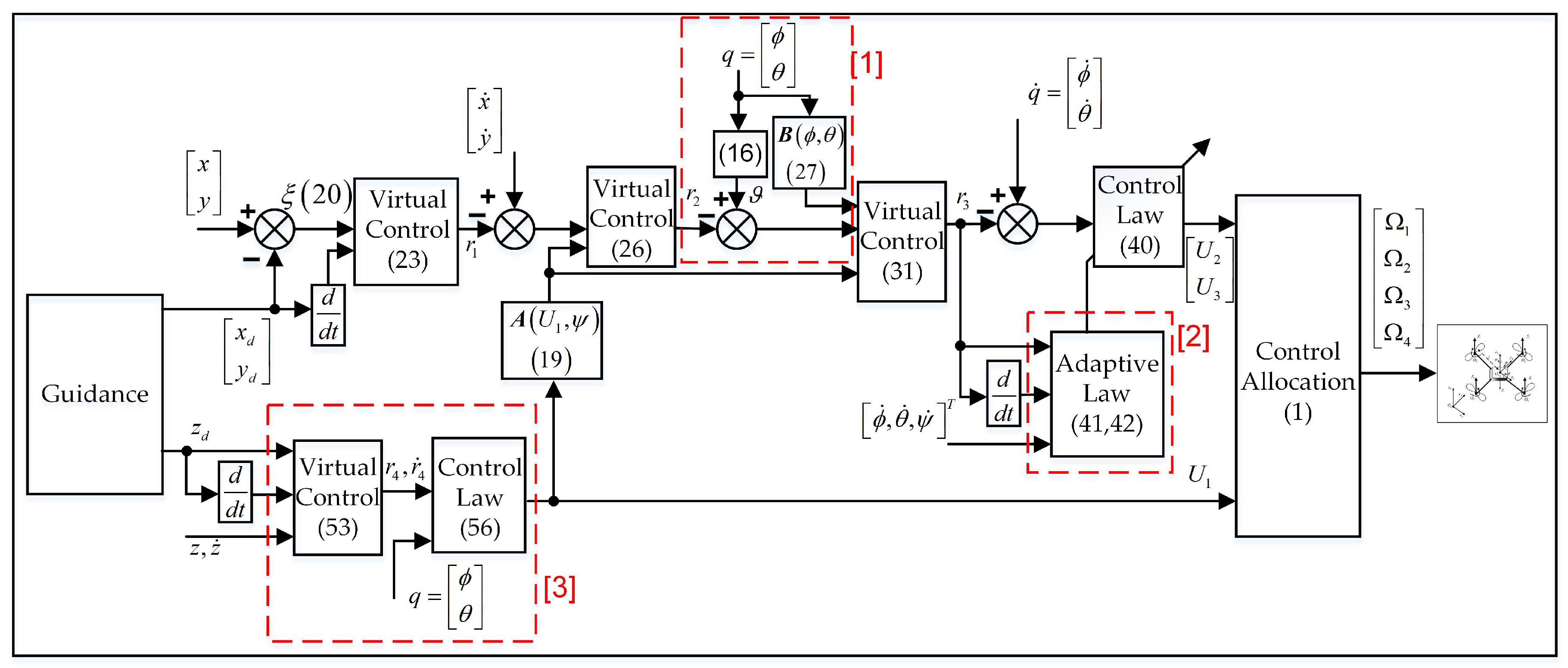
The control diagram of the proposed control and adaptive law is shown in Figure 2 to certainly show our contributions in three red boxes. In the box [1], the virtual control $r_2$ and a new variable $\vartheta$ are presented to clearly describe the relationship between two loops of the horizontal subsystem. Additionally, there is a new adaptive law to estimate several unknown parameters such as inertial moment, arm length, and drag moment coefficients in the box [2]. Finally, the box [3] shows the proposed altitude controller which forces the tracking error to lie in its boundary to ensure the safety of this system.

After determining the desired trajectory, the guidance function separates that into two movements, i.e., horizontal $\left(x_d,y_d\right)$ and vertical $z_d$ motions. The proposed horizontal and altitude controllers receive their references to provide the independent control inputs. In horizontal flow, the virtual input $r_1$ is calculated by combining tracking error $\xi$ and the time-derivative of reference in (23). At the next stage, by using the matrix $A(U_1,\psi )$ (19), $r_1$, and the horizontal velocities, virtual control $r_2$ (26) is obtained to become the input of the aforementioned box [1]. After finding virtual control $r_3$ (31), the proposed adaptive law in the mentioned box [2] (41) and (42) cooperatives with $r_3$ and angular rate $\dot{q}$ to obtain the intermediate control law (40). On the other hand, altitude controller $U_1$ (56) is calculated by combining the virtual input $r_4$ (53) and Euler angle q. The final block-control allocation (1) automatically generates four different rotors speeds ${\mathsf{\Omega }}_i$ ($i=\overline{1,4}$) to meet the requirements based on trajectory tracking.

4. Numerical Results

In order to verify the proposed method in this paper, we evaluate the simulation results of the Unmanned Aerial Vehicle–Quadcopter following several desired tracking trajectories. The parameters of the proposed system are given as: $m=1.568$ kg, $I_{xx}=I_{yy}=0.0119$ kg·m${}^2$, $I_{zz}=0.0223$ kg·m${}^2$, $g=9.8$ m/s${}^2$, $b=7.73\times {10}^{-6}$ Ns${}^2$, $d=1.28\times {10}^{-7}$ Nms${}^2$, ${\mu }_1={\mu }_2={\mu }_3=0.1$ s${}^{-1}$ and the initial states are chosen such that an initial position of the quadcopter lies outside the desired trajectory to strongly verify the proposed method: $x\left(0\right)=0.5$ m, $y\left(0\right)=0.5$ m, $z\left(0\right)=0$ m, $\varphi \left(0\right)=\theta \left(0\right)=\psi \left(0\right)=0$ rad, $x_d\left(0\right)=0$ m, $y_d\left(0\right)=0$ m, $z_d\left(0\right)=0$ m, $\widehat{\mathsf{\Gamma }}\left(0\right)={\left[1,1,1,1\right]}^T$, vec$\left(\widehat{E}\right)={\left[0.5,0.5,0.5,0.5\right]}^T$. Based on the proposed Theorem 1, the matrix and scalar coefficients are selected as follows: ${\mathbf{K}}_1={\mathbf{I}}_2$, ${\mathbf{K}}_2=2{\mathbf{I}}_2$, ${\mathbf{K}}_3=3{\mathbf{I}}_2$, ${\mathbf{K}}_4=16{\mathbf{I}}_2$, $k_5=6$, $k_6=5$, $ϵ=0.2$, ${\mathbf{Q}}_1=10{\mathbf{I}}_4$, ${\mathbf{Q}}_2=4{\mathbf{I}}_4$.

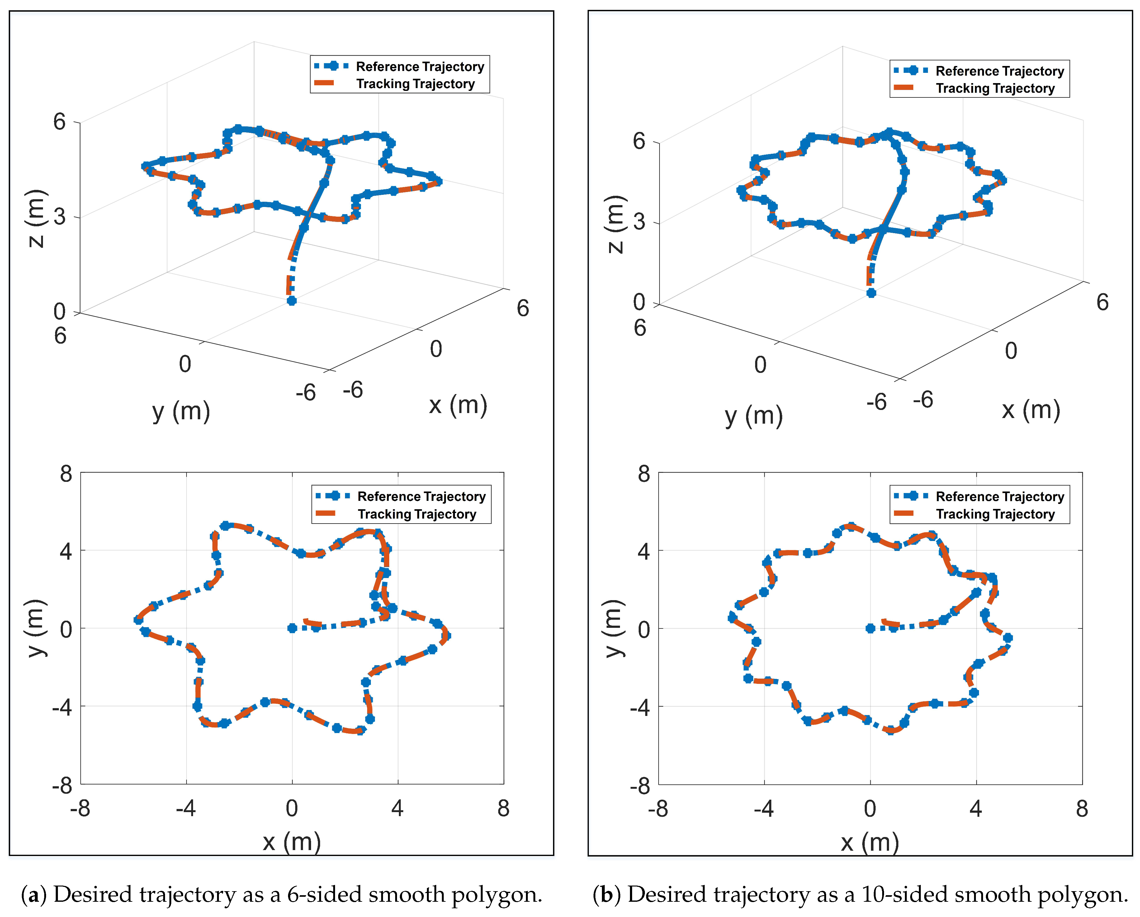
The simulation scenarios involve several flying shapes in the air from where the initial position does not belong to these desired paths. The objective is that the investigated system should be able to track given trajectories using finite time simulation and satisfying Assumption 2. To generate several complicated orbits, the desired $\eta$ polygon horizontal trajectory is created in two-dimensional space [27] as follows:

$$\begin{array}{cc}\hfill x_d& =a\left[R+cos\left(\eta \omega t\right)\right]cos\left(\omega t\right)\hfill \\ \hfill y_d& =a\left[R+cos\left(\eta \omega t\right)\right]sin\left(\omega t\right)\hfill \\ \hfill z_d& =\left[h_d-z\left(0\right)\right]\left(1-e^{-\omega t}\right)+z\left(0\right)\hfill \end{array}$$

(58)

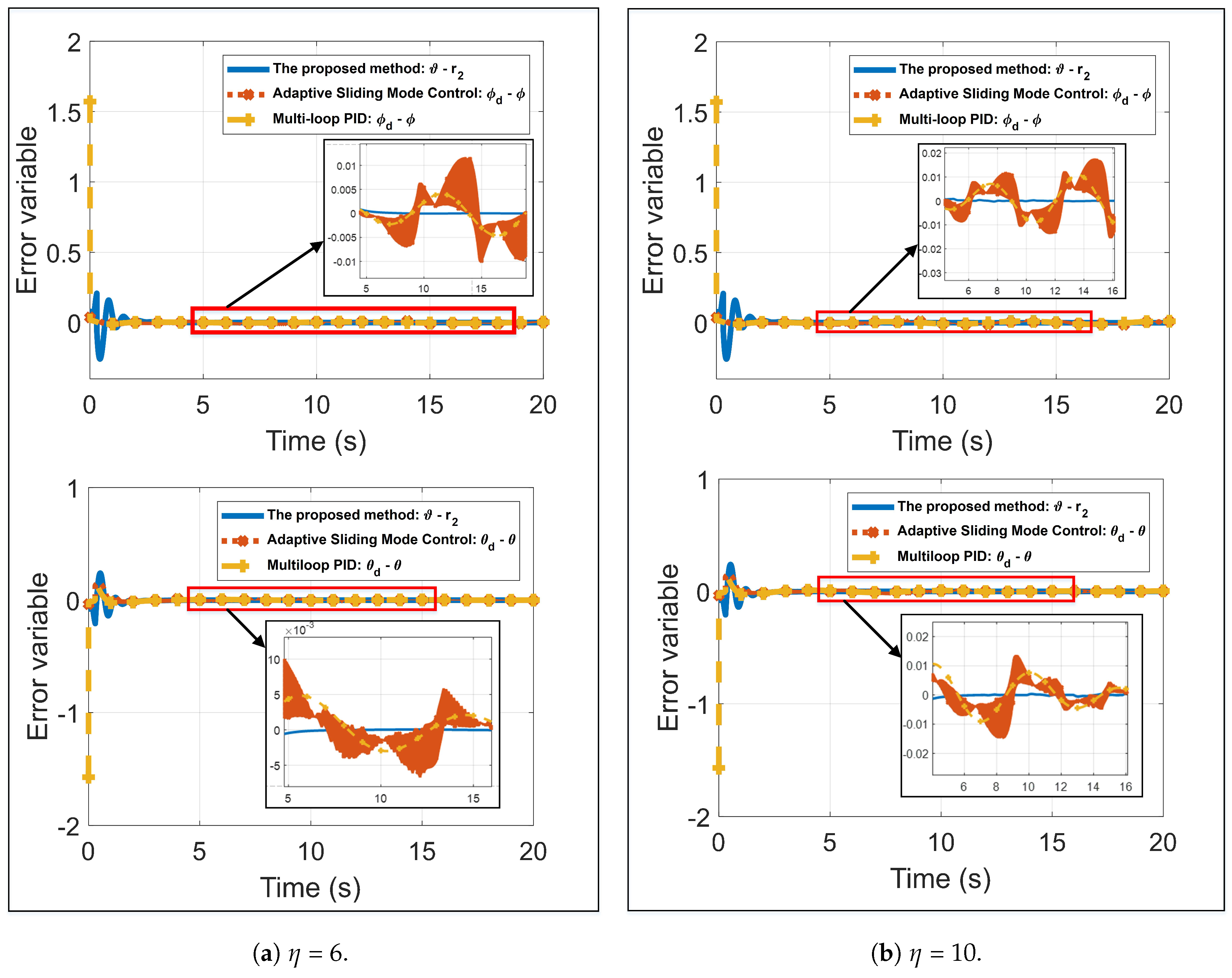
where a, $\omega$, and R are the scale, the angular velocity, and radius of the desired trajectory, respectively. They were set to $a=2.5$, $\omega =0.5$ rad/s, and $R=1$ m. It can be observed that the reference trajectories can be generated by changing $\eta$ in (58) to obtain $\eta$-sided smooth polygon. We either set $\eta =6$ (Figure 3a) or $\eta =10$ (Figure 3b) in $xyz$-space and $xy$-plane and desired altitude $h_d=4$ m to generate two reference shapes to verify the proposed approach. Additionally, to emphasize the effectiveness of the proposed scheme, the adaptive sliding mode control [25] and Multi-loop PID [46] are also applied to this tracking problem. These methods show that the position and attitude subsystems are guaranteed to be in stability by two separated controllers, but there is not any relationship between these two loops. Therefore, we expect our method presented in the red box [1] in Figure 3a to be able to cope with issue.

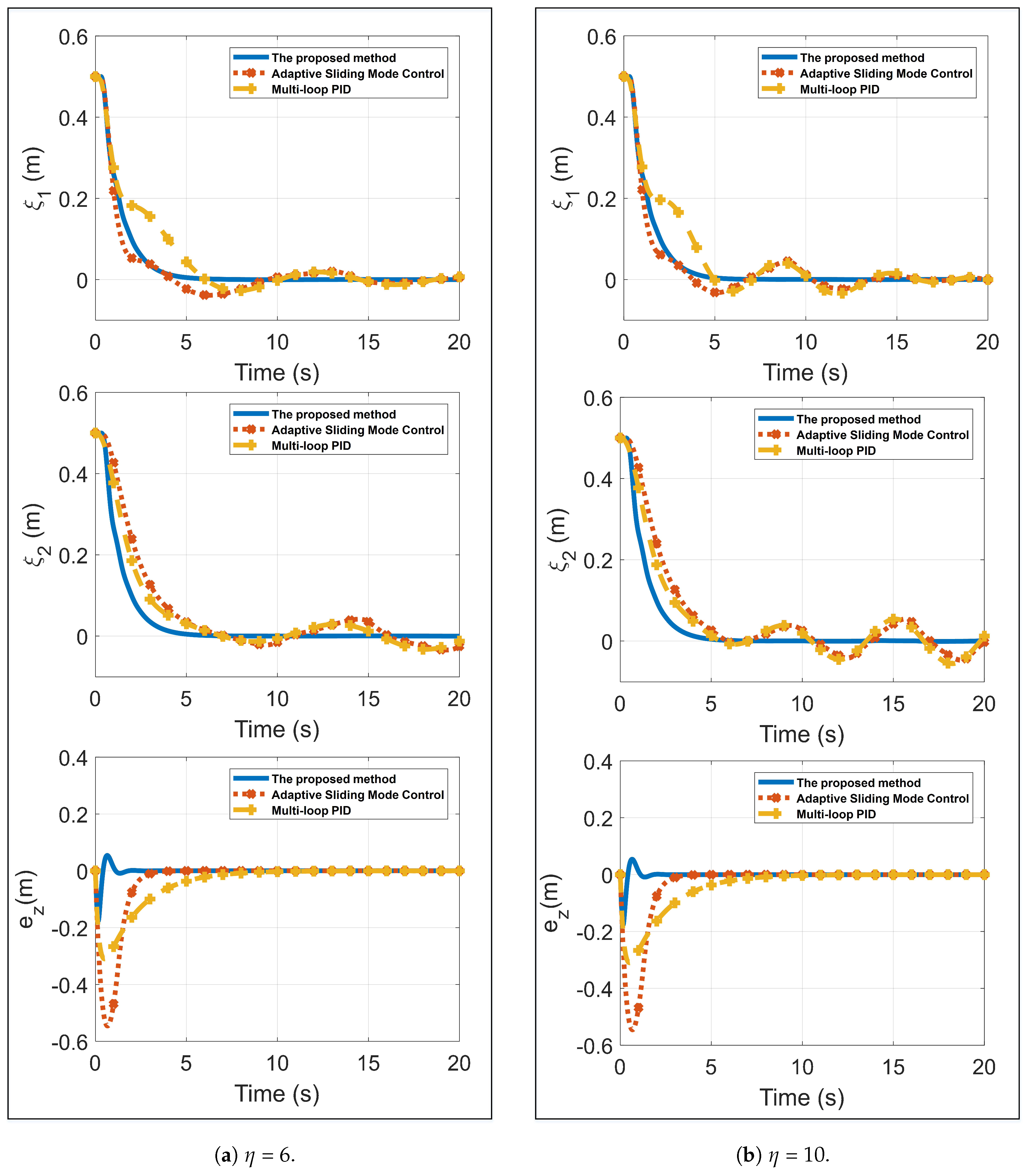
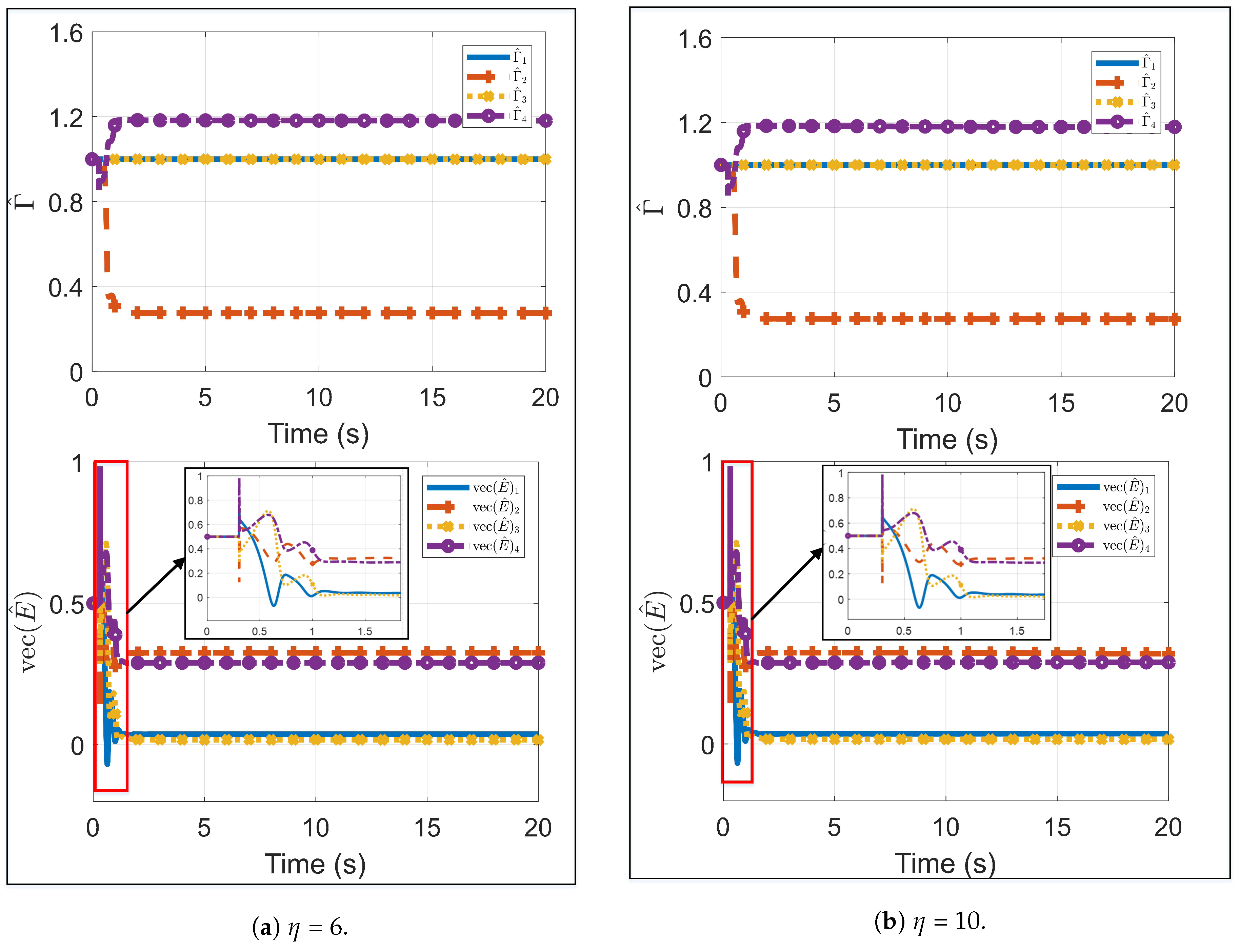
Figure 4a,b compares the performance of three different approaches which include the proposed method, adaptive sliding mode control, and Multi-loop PID. Having started from the same initial state, the 3D position tracking errors tend towards the origin. If we increase the model parameters by 30% to investigate the system robustness, only the blue solid line asymptotically converges to the origin because of the proposed adaptive law. The estimated values of $\mathsf{\Gamma },\mathbf{E}$ in Figure 5a,b become constant as time goes to infinity, which verifies our Theorem 1. The remaining curves exhibit oscillations in the tracking errors along the x and y-axes from the fifth to the twentieth second. Moreover, when it comes to considering the z-axis, the error of altitude tracking asymptotically converges to the origin and is always limited by $ϵ$ in (46) to ensure Assumption 2.

Figure 6a,b compares the errors between position and attitude subsystems in terms of three different methods. Most of the previous studies tended to divide the horizontal subsystem into position and attitude parts to separately design a control law, which may cause a finite escape time. These figures confirm that this undesirable phenomenon which is mentioned in Remark 1 does not appear to guarantee the globally asymptotic stability of the proposed scheme. The authors in [25] employed an adaptive sliding mode control to achieve fast response for the attitude subsystem in an effort to avoid the finite escape time. However, this approach definitely created a chattering phenomenon which may cause damage to the practical system. While the dotted line responds to the reference trajectory slower than the dashed line to prevent chattering to obtain better tracking performance, there is a finite escape time at initial state. It can be seen that responses of the both adaptive SMC and multi-loop PID gradually chatter and oscillate around zero, which cannot be able to achieve asymptotic stability. In contrast, the proposed method prevents either weakness from occurring in Figure 6a,b. Because the proposed adaptive law requires a small time interval depending on matrix ${\mathbf{Q}}_1$ and ${\mathbf{Q}}_2$ to estimate unknown parameters (Figure 5a,b), the errors/solid lines between a new proposed variable $\vartheta$ and a virtual control input $r_2$ rapidly fluctuating around zero before asymptotically converging to the origin during ten seconds from the fifth second. By reviewing the Figure 4a,b, Figure 5a,b, and Figure 6a,b, we can validate the effectiveness of the proposed Theorem 1.

5. Conclusions

In conclusion, a theoretical constructive scheme of the quadcopter in three-dimensional space has been proposed to carry out the trajectory tracking problem in the presence of uncertain parameters. Additionally, this method is able to eliminate the finite escape time when separating the mathematical model into several subsystems and to allow smooth altitude changes. In order to design the horizontal and altitude controllers, our approach parallelly separates the mathematical model of the investigated quadcopter into horizontal and vertical subsystems. The main successes of this paper include: (1) we have modified the use of backstepping technique to integrate position and attitude submodels for the horizontal control law, which theoretically demonstrates the asymptotic stability of the entire horizontal subsystem; (2) we have proposed an adaptive law to estimate several unknown parameters such as arm length, inertial moment, and viscous coefficients which are difficult to be accurately calculated in practice to obtain the constant values that automatically adjust the aforementioned horizontal controller. By invoking the LaSalle’s theorem, the horizontal tracking error is asymptotically stable and the suitable parameter estimator is stable; and (3) we have applied the barrier Lyapunov function to guarantee the altitude tracking error to be within the pre-specified bound, which ensures that the vehicle’s vertical descending acceleration does not exceed the gravitational acceleration. Through simulation comparison with the existing studies, we could verify the effectiveness of and superior performance of our method with regard to path tracking. In future work, we plan to combine several quadcopter models or quadcopter with other ground robots to extend this proposed approach to become a cooperative system.

References

- Mogili, U.R.; Deepak, B.B.V.L. Review on application of drone systems in precision agriculture. Procedia Comput. Sci. 2018, 133, 502–509. [Google Scholar] [CrossRef]
- Yallappa, D.; Veerangouda, M.; Maski, D.; Palled, V.; Bheemanna, M. Development and evaluation of drone mounted sprayer for pesticide applications to crops. In Proceedings of the IEEE Global Humanitarian Technology Conference, San Jose, CA, USA, 19–22 October 2017; pp. 1–7. [Google Scholar]
- Suprapto, B.Y.; Heryanto, M.A.; Suprijono, H.; Muliadi, J.; Kusumoputro, B. Design and development of heavy-lift hexacopter for heavy payload. In Proceedings of the International Seminar on Application for Technology of Information and Communication, Semarang, Indonesia, 7–8 October 2017; pp. 242–247. [Google Scholar]
- Benito, J.A.; Glez-de-Rivera, G.; Garrido, J.; Ponticelli, R. Design considerations of a small UAV platform carrying medium payloads. In Proceedings of the Design of Circuits and Integrated Systems, Madrid, Spain, 26–28 November 2014; pp. 1–6. [Google Scholar]
- Naidoo, Y.; Stopforth, R.; Bright, G. Development of an UAV for search & rescue applications. In Proceedings of the IEEE Africon’11, Livingstone, Zambia, 13–15 September 2011; pp. 1–6. [Google Scholar]
- Erdos, D.; Erdos, A.; Watkins, S.E. An experimental UAV system for search and rescue challenge. IEEE Aerosp. Electron. Syst. Mag. 2013, 28, 32–37. [Google Scholar] [CrossRef]
- Mustapa, Z.; Saat, S.; Husin, S.H.; Abas, N. Altitude controller design for multi-copter UAV. In Proceedings of the 2014 International Conference on Computer, Communications, and Control Technology (I4CT), Langkawi, Malaysia, 2–4 September 2014; pp. 382–387. [Google Scholar]
- Santos, M.F.; Pereira, V.S.; Ribeiro, A.C.; Silva, M.F.; Vidal, M.J.D.C.V.F.; Honorio, L.M.; Cerqueira, A.S.; Oliveira, E.J. Simulation and comparison between a linear and nonlinear technique applied to altitude control in quadcopters. In Proceedings of the 18th International Carpathian Control Conference (ICCC), Sinaia, Romania, 28–31 May 2017; pp. 234–239. [Google Scholar]
- Pounds, P.E.I.; Bersak, D.R.; Dollar, A.M. Stability of small-scale UAV helicopters and quadrotors with added payload mass under PID control. Autonom. Rob. 2012, 33, 129–142. [Google Scholar] [CrossRef]
- Salih, A.L.; Moghavvemi, M.; Mohamed, H.A.F.; Gaeid, K.F. Modelling and PID controller design for a quadrotor unmanned air vehicle. In Proceedings of the IEEE International Conference on Automation, Quality and Testing, Robotics (AQTR), Cluj-Napoca, Romania, 28–30 May 2010. [Google Scholar]
- Xuan-Mung, N.; Hong, S.K. Improved Altitude Control Algorithm for Quadcopter Unmanned Aerial Vehicles. Appl. Sci. 2019, 9, 2122. [Google Scholar] [CrossRef]
- Modelling and Control of Quadcopter. Available online: https://www.researchgate.net/file.PostFileLoader.html?id=576d16ed93553b24b5721a9a&assetKey=AS%3A376462596165634%401466767085787 (accessed on 12 September 2019).
- Li, J.; Li, Y. Dynamic analysis and PID control for a quadrotor. In Proceedings of the IEEE International Conference on Mechatronics and Automation, Beijing, China, 7–10 August 2011. [Google Scholar]
- Ahmed, A.H.; Ouda, A.N.; Kamel, A.M.; Elhalwagy, Y.Z. Attitude stabilization and altitude control of quadrotor. In Proceedings of the 12th International Computer Engineering Conference (ICENCO), Cairo, Egypt, 28–29 December 2016. [Google Scholar]
- Khan, H.S.; Kadri, M.B. Attitude and altitude control of quadrotor by discrete PID control and non-linear model Predictive control. In Proceedings of the International Conference on Information and Communication Technologies (ICICT), Karachi, Pakistan, 12–13 December 2015. [Google Scholar]
- Bolandi, H.; Rezaei, M.; Mohsenipour, R.; Nemati, H.; Smailzadeh, S.M. Attitude control of a quadrotor with optimized PID controller. Intell. Control Autom. 2013, 4, 335–342. [Google Scholar] [CrossRef]
- Thanh, H.L.N.N.; Hong, S.K. Quadcopter robust adaptive second order sliding mode control based on PID sliding surface. IEEE Access 2018, 6, 66850–66860. [Google Scholar] [CrossRef]
- Thanh, H.L.N.N.; Nguyen, N.P.; Hong, S.K. Simple nonlinear control of quadcopter for collision avoidance based on geometric approach in static environment. Int. J. Adv. Rob. Syst. 2018, 15. [Google Scholar] [CrossRef] [Green Version]
- Nguyen, N.P.; Hong, S.K. Fault-tolerant Control of Quadcopter UAVs Using Robust Adaptive Sliding Mode Approach. Energies 2018, 12, 95. [Google Scholar] [CrossRef]
- Mian, A.A.; Daobo, W. Modeling and backstepping-based nonlinear control strategy for a 6 DOF quadrotor helicopter. Chin. J. Aeronaut. 2008, 21, 261–268. [Google Scholar] [CrossRef]
- Paiva, E.; Soto, J.; Salinas, J.; Ipanaqué, W. Modeling, simulation and implementation of a modified PID controller for stabilizing a quadcopter. In Proceeding of the IEEE International Conference on Automatica, Curico, Chile, 19–21 October 2016; pp. 1–6. [Google Scholar]
- Bouabdallah, S.; Noth, A.; Siegwart, R. PID vs LQ control techniques applied to an indoor micro quadrotor. In Proceeding of the International Conference on Intelligent Robots and Systems, Sendai, Japan, 28 September–2 October 2004; pp. 2451–2456. [Google Scholar]
- Argentim, L.M.; Rezende, W.C.; Santos, P.E.; Aguiar, R.A. PID, LQR and LQR-PID on a quadcopter platform. In Proceedings of the International Conference on Informatics, Electronics and Vision, Dhaka, Bangladesh, 17–18 May 2013; pp. 1–6. [Google Scholar]
- Li, S.; Li, B.; Geng, Q. Adaptive sliding mode control for quadrotor helicopters. In Proceeding of the 33rd Chinese Control Conference, Nanjing, China, 28–30 July 2014; pp. 71–76. [Google Scholar]
- Nadda, S.; Swarup, A. On adaptive sliding mode control for improved quadrotor tracking. J. Vibr. Control 2018, 24, 3219–3230. [Google Scholar] [CrossRef]
- Binh, N.T.; Tung, N.A.; Nam, D.P.; Huong, N.T.V. Robust Adaptive Backstepping in Tracking Control for Wheeled Inverted Pendulum. In Information Systems Design and Intelligent Applications; Springer: Singapore, 2018; pp. 423–434. [Google Scholar]
- Binh, N.T.; Tung, N.A.; Nam, D.P.; Quang, N.H. An Adaptive Backstepping Trajectory Tracking Control of a Tractor Trailer Wheeled Mobile Robot. Int. J. Control Autom. Syst. 2019, 17, 465–473. [Google Scholar] [CrossRef]
- Madani, T.; Benallegue, A. Backstepping control for a quadrotor helicopter. In Proceeding of the IEEE/RSJ International Conference on Intelligent Robots and Systems, Beijing, China, 9–15 October 2006; pp. 3255–3260. [Google Scholar]
- Das, A.; Lewis, F.; Subbarao, K. Backstepping approach for controlling a quadrotor using lagrange form dynamics. J. Intell. Rob. Syst. 2009, 56, 127–151. [Google Scholar] [CrossRef]
- Ramirez-Rodriguez, H.; Parra-Vega, V.; Sanchez-Orta, A.; Garcia-Salazar, O. Robust backstepping control based on integral sliding modes for tracking of quadrotors. J. Intell. Rob. Syst. 2014, 73, 51–66. [Google Scholar] [CrossRef]
- Zuo, Z. Adaptive trajectory tracking control design with command filtered compensation for a quadrotor. J. Vibr. Control 2013, 19, 94–108. [Google Scholar] [CrossRef]
- Do, K.D. Path–tracking control of stochastic quadrotor aircraft in three–dimensional space. J. Dyn. Syst. Meas. Control 2015, 137, 101003. [Google Scholar] [CrossRef]
- Krstic, M.; Kanellakopoulos, I.; Kokotovic, P.V. Nonlinear and Adaptive Control Design; Wiley: New York, NY, USA, 1995. [Google Scholar]
- Alexis, K.; Nikolakopoulos, G.; Tzes, A. Model predictive quadrotor control: Attitude, altitude and position experimental studies. IET Control Theory Appl. 2012, 6, 1812–1827. [Google Scholar] [CrossRef]
- Ru, P.; Subbarao, K. Nonlinear model predictive control for unmanned aerial vehicles. Aerospace 2017, 4, 31. [Google Scholar] [CrossRef]
- Raffo, G.V.; Ortega, M.G.; Rubio, F.R. An integral predictive/nonlinear H∞ control structure for a quadrotor helicopter. Automatica 2010, 46, 29–39. [Google Scholar] [CrossRef]
- Gong, X.; Hou, Z.C.; Zhao, C.J.; Bai, Y.; Tian, Y.T. Adaptive backstepping sliding mode trajectory tracking control for a quad-rotor. Int. J. Autom. Comput. 2012, 9, 555–560. [Google Scholar] [CrossRef]
- Mofid, O.; Mobayen, S. Adaptive sliding mode control for finite-time stability of quad-rotor UAVs with parametric uncertainties. ISA Trans. 2018, 72, 1–14. [Google Scholar] [CrossRef]
- Li, S.; Wang, Y.; Tan, J.; Zheng, Y. Adaptive RBFNNs/integral sliding mode control for a quadrotor aircraft. Neurocomputing 2016, 216, 126–134. [Google Scholar] [CrossRef]
- Boudjedir, H.; Bouhali, O.; Rizoug, N. Adaptive neural network control based on neural observer for quadrotor unmanned aerial vehicle. Adv. Rob. 2014, 28, 1151–1164. [Google Scholar] [CrossRef]
- Fei, J.; Lu, C. Adaptive sliding mode control of dynamic systems using double loop recurrent neural network structure. IEEE Trans. Neural Netw. Learn. Syst. 2017, 29, 1275–1286. [Google Scholar] [CrossRef]
- Gao, H.; Liu, C.; Guo, D.; Liu, J. Fuzzy adaptive PD control for quadrotor helicopter. In Proceedings of the 2015 IEEE International Conference on Cyber Technology in Automation, Control, and Intelligent Systems (CYBER), Shenyang, China, 8–12 June 2015; pp. 281–286. [Google Scholar]
- Nadda, S.; Swarup, A. Improved quadrotor altitude control design using second–order sliding mode. J. Aerosp. Eng. 2017, 30, 04017065. [Google Scholar] [CrossRef]
- Khalil, H.K. Nonlinear Systems, 3rd ed.; Prentice Hall: New York, NY, USA, 2002. [Google Scholar]
- Tee, K.P.; Ge, S.S.; Tay, E.H. Barrier Lyapunov functions for the control of output-constrained nonlinear systems. Automatica 2009, 45, 918–927. [Google Scholar] [CrossRef]
- Copter Attitude Control. Available online: http://ardupilot.org/dev/docs/apmcopter-programming-attitude-control-2.html (accessed on 12 September 2019).
Figure 1.
Plus-Configuration of a quadcopter.
Figure 2.
Control diagram of the proposed method.
Figure 3.
Trajectory tracking performance of the proposed method in the xyz-space and xy-plane.
Figure 4.
Comparison of tracking error performance between our method and existing approaches.
Figure 5.
The estimated unknown parameters of the proposed method.
Figure 6.
Comparison of two loops’ error variables between our method and existing approaches.