Insider Threat Detection Based on User Behavior Modeling and Anomaly Detection Algorithms

Abstract

Insider threats are malicious activities by authorized users, such as theft of intellectual property or security information, fraud, and sabotage. Although the number of insider threats is much lower than external network attacks, insider threats can cause extensive damage. As insiders are very familiar with an organization’s system, it is very difficult to detect their malicious behavior. Traditional insider-threat detection methods focus on rule-based approaches built by domain experts, but they are neither flexible nor robust. In this paper, we propose insider-threat detection methods based on user behavior modeling and anomaly detection algorithms. Based on user log data, we constructed three types of datasets: user’s daily activity summary, e-mail contents topic distribution, and user’s weekly e-mail communication history. Then, we applied four anomaly detection algorithms and their combinations to detect malicious activities. Experimental results indicate that the proposed framework can work well for imbalanced datasets in which there are only a few insider threats and where no domain experts’ knowledge is provided.

1. Introduction

Insider threat is a security issue that arises from persons who have access to a corporate network, systems, and data, such as employees and trusted partners [1]. Although insider threats do not occur frequently, the magnitude of damage is greater than from external intrusions [2,3]. Because insiders are very familiar with their organization’s computer systems and operational processes, and have the authorization to use these systems, it is difficult to determine when they behave maliciously [4]. Many system protection technologies have been developed against intrusions attempted by outsiders, e.g., quantifying the pattern of connection Internet protocols (IPs) and types of attacks [5]. However, past research on the security of a company’s internal information has mainly focused on detecting and preventing intrusion from the outside, and few studies have addressed methods to detect insider threats [6].

There are three research mainstream strategies for insider threat detection. The first strategy is to develop a rule-based detection system [7,8]. In this strategy, a pool of experts generates a set of rules to identify insiders’ malicious activities. Then, each user’s behavior is recorded as a log and is tested to determine whether it meets any of the pre-designed rules. Cappelli et al. [9] discussed the types of insider threats and domain knowledge to prevent/detect insider threats. Rule-based detection methods have a critical limitation in that the rules must be constantly updated through the knowledge of domain experts, so the risk of someone circumventing the rules always exists [10]. Hence, rule-based methods based on expert knowledge are inflexible to changing insider threats methods, which results in unsatisfactory detection performance [7,10,11].

The second strategy is to build a network graph to identify suspicious users or malicious behaviors by monitoring the changes of the graph structure [12]. Graph-based insider threat identification does not only analyze the value of the data itself but also analyzes the relationships among the data. The relationships among the data are represented by edges connecting the nodes of the graph, and its properties can be analyzed to determine the relationships of specific nodes to insider threats. Eberle et al. [12] defined an abnormal activity if modifications, insertions, or deletions occur in the underlying structure of a normal data graph. To determine the structure of a normal data graph, they employed a graph-based knowledge discovery system called “SUBDUE”. Parveen et al. [13] used graph-based anomaly detection (GBAD)-MDL, GBAD-P and GBAD-MPS to determine the ideal structure of a graph, and added an ensemble-based approach to detect abnormal insider activities in the “1998 Lincoln Laboratory Intrusion Detection” dataset.

The third strategy is to build a statistical or machine learning model based on previous data to predict potential malicious behavior [14]. Machine learning is a methodology in which a computer learns an algorithm to optimize appropriate performance criteria from training data to perform given tasks [15]. Insider threat detection using machine learning aims at developing a method to automatically identify users who perform unusual activities among all users without prior knowledge or rules. Because the machine learning methodology can continuously learn and update the algorithms from the data, it can perform stable and accurate detection compared to rule-based detection. Gavai et al. [16] employed random forest [17] and isolation forest [18] to classify retirees for the ‘Vegas’ dataset, in which behavior features are extracted from e-mail transmission patterns and contents, logon and logoff records, web browsing patterns, and file access patterns. Ted et al. [4] collected user activity data for 5500 users using a tool called “SureView” (Forcepoint, Austin, TX, USA). They extracted features from the data by considering potential malicious activity scenarios by insiders, implied abnormal activities, temporal order, and high-level statistical patterns. They created variables involving insider’s various actions such as email, files, and logons, and they applied 15 statistical indices and various machine-learning algorithms to determine the most suitable combination of algorithms. Eldardiry et al. [10] detected insider threats by measuring similarity in behavior between the role group to which a user actually belongs and another role group to which he/she does not belong, assuming that users in the same role groups have similar patterns of activities.

Although the learning model-based strategy is advantageous in that it does not depend on the knowledge of domain experts to define a set of rules or to construct a relational graph, it has two practical obstacles: (1) the way of quantifying a user’s behavioral data and (2) the lack of abnormal cases available for model building. As most statistical/machine learning models take a continuous value as an input to the detection model, each user’s behavior during a certain period (e.g., day) should be transformed into a numerical vector in which each element represents a specific behavioral characteristic. Because a user’s behavior can be extracted from different data sources, such as systems usage logs, e-mail sending and receiving networks, and e-mail contents, one of the key points of building successful insider threat detection models is to define useful features for different types of data and to transform the unstructured raw data into a structured dataset. From a modeling perspective, it is virtually impossible to train a binary classification algorithm when only a few abnormal examples exist [19]. Under this class imbalance circumstance, most statistical/machine learning algorithms tend to classify all activities as normal, which results in a useless insider-threat detection model. To resolve these shortcomings, we propose an insider-threat detection framework based on user activity modeling and one-class classification. During the user activity modeling stage, we consider three types of data. First, all activity logs of individual users recorded in the corporate system are collected. Then, candidate features are extracted by summarizing specific activities. For example, if the system logs contain information on when a user connects his/her personal Universal serial bus (USB) drive to the system, the total number of USB connections per day can be extracted as a candidate variable. Second, we consider user-generated contents, such as the body of an e-mail, to create candidate features. Specifically, we used topic modeling to convert unstructured text data to a structured vector while preserving the meaning of text as much as possible. Lastly, we construct a communication network of users based on e-mail exchange records. Then, summary statistics for a node including centrality indices are computed and used as candidate features. During the insider-threat detection model-building stage, we employ one-class classification algorithms to learn the characteristics of normal activities based on three categories of candidate feature sets. We then employ four individual one-class classification algorithms and exploit the possible advantages of their combinations. By considering heterogeneous feature sets, we expect an improved detection performance compared to detection models based on a single dataset. In addition, by employing one-class classification algorithms, it becomes practically possible to build an insider-threat detection model without the need for past abnormal records.

The rest of this paper is organized as follows. In Section 2, we introduce the dataset used in this study and demonstrate user activity modeling, i.e., how to transform unstructured logs or contents to a structured dataset. In Section 3, we introduce the one-class classification algorithms employed to build the insider-threat detection model. In Section 4, experimental results are demonstrated with some interesting observations. Finally, in Section 5, we conclude our study with some future research directions.

2. Dataset and User Activity Modeling

In this section, we briefly introduce the dataset used in our study. Then, we demonstrate how we define candidate features for the insider-threat detection model and how we transform three different types of user activity data into numeric vectors.

2.1. CERT Dataset

Because it is very difficult to obtain actual corporate system logs, we used the “CERT Insider Threat Tools” dataset (Carnegie Mellon’s Software Engineering Institute, Pittsburgh, PA, USA) [20]. The CERT dataset is not real-world enterprise data, but it is an artificially generated dataset created for the purpose of validating insider-threat detection frameworks [1].

The CERT dataset includes employee computer usage logs (logon, device, http, file, and email) with some organizational information such as employee departments and roles. Each table consists of columns related to a user’s ID, timestamps, and activities. The CERT dataset has six major versions (R1 to R6) and the latest version has two variations: R6.1 and R6.2. The types of usage information, number of variables, number of employees, and number of malicious insider activities are different depending on the dataset version. We conducted this study using R6.2, which is the latest and largest dataset. In this version, the dataset includes 4000 users, among whom only five users behaved maliciously. The description of the logon activity table is provided in

Table 1. Log records of logon activities.

Recorded Item	Description
ID	Primary key of an observation
Date	Day/Month/Year
User	User ID
Personal computer (PC)	Key number of a PC logged on
Activity	Log on or log off (Binary type)

and the other activities are provided in the Appendix A,

Table A1. User behavior log records of computer activities in the CERT dataset.

	Recorded Item	Description
File	ID	Primary key
	Date	Day/Month/Year Hour:Min:Sec
	User	Primary key of a user
	PC	Primary key of a PC
	Filename	File directory
	Activity	File Open/Write/Copy/Delete
	To_removable_media	Data PC to Removable media (TRUE, FALSE)
	From_removable_media	Data Removable media to PC (TRUE, FALSE)
	Content	Hexadecimal encoded file header and contents text
Device	ID	Primary key of an observation
	Date	Day/Month/Year Hour:Min:Sec
	User	User ID
	PC	Key number of a PC logged on
	File tree	File directory
	Activity	Log on or log off (Binary type)
HTTP	ID	Primary key
	Date	Day/Month/Year Hour:Min:Sec
	User	Primary key of a user
	PC	Primary key of a PC
	URL	URL address
	Activity	Activity (Visit/Upload/Download)
	Content	Content of a URL
Email	ID	Primary key of an observation
	Date	Day/Month/Year Hour:Min:Sec
	User	Primary key of a user
	PC	Primary key of a PC
	To	Receiver
	Cc	Carbon copy
	Bcc	Blind carbon copy
	From	Sender
	Activity	Activity (Send/Receive)
	Size	Size of an email
	Attachments	Attachment file name
	Content	Content of an email
Psychometric	Employee name	Employee name
	User ID	ID of an employee
	O	Openness to experience
	C	Conscientiousness
	E	Extraversion
	A	Agreeableness
	N	Neuroticism
LDAP	Employee name	Employee name
	User ID	ID of a user
	Email	Email address
	Role	Role of a user
	Project	Project participation
	Business unit	Business unit
	Functional unit	Functional unit
	Department	Department
	Team	Team
	Supervisor	Supervisor
Decoy file	Decoy filename	Decoy file directory
		Name and extension
	PC	PC name

.

2.2. User Activity Modeling Based on Daily Activity Summaries

In the CERT dataset, user behaviors are stored in five data tables: logon, USB, http, file, and email. To comprehensively utilize heterogeneous user behavior data, it is necessary to integrate the behavioral information into one standardized data table in chronological order. Because the proposed user-level insider-threat detection models developed in this study work on a daily or weekly basis, we first integrated a user’s fragmented activity records for each day and summarized them to quantify the intensity of activity, which becomes an input variable in the detection model. For example, based on the information stored in the logon table, it is possible to extract the number of times a user has logged on to the computer during a specific day.

To determine candidate input variables for insider-threat detection, we examined the input variables used in past studies, as shown in

Table 2. Referred articles for variable selection.

Research Papers	Authors	Year
Supervised and unsupervised methods to detect insider threat from enterprise and online activity data	Gavai et al. [16]	2015
Detecting insider threats using ben-ware: beneficial intelligent software for identifying anomalous human behavior	McGough et al. [21]	2015
Multi-source fusion for anomaly detection: using across-domain and across-time peer-group consistency checks	Eldardiry et al. [10]	2014
Use of domain knowledge to detect insider threats in computer activities	Young et al. [22]	2013
Insider threat simulation and performance analysis of insider detection algorithms with role-based models	Nellikar [23]	2010

. From these references, we created all possible input variables that can be extracted from the CERT dataset. The total number of candidate input variables is 60 and the description of each variable is provided in the Appendix A,

Table A2. List of variables extracted from integrated daily activities.

	Variable Name	Description
Base	user	User ID
	date	Date
	workingday	Working day or not (Binary type)
Logon	numlogonDay	Number of logons on working hours
	numlogonNight	Number of logons on off-hours
	numlogoffDay	Number of logoffs on working hours
	numlogoffNight	Number of logoffs on off-hours
	numPClogonDay	Number of s PC logons on working hour
	numPClogonNight	Number of PC logons on off-hours
	numPClogoffDay	Number of PC logoffs on working hour
	numPClogoffNight	Number of PC logoffs on off-hours
	onoffNotsameDay	Counts of the number of logons and logoffs are not the same on working hours
	onoffNotsameNight	Counts of the number of logons and logoffs are not the same on off-hours
Device	numPCwithUSBDay	Number of PC that uses USB device on working hours
	numPCwithUSBNight	Number of PC that uses USB device on off-hours
	numConnectionDay	Number of connections with devices on working hours
	numConnectionNight	Number of connections with devices on off-hours
	numCopy2DeviceDay	Number of copied files from PC to devices on working hours
	numCopy2DeviceNight	Number of copied files from PC to devices on off-hours
	numWrite2DeviceDay	Number of written files from PC to devices on working hours
	numWrite2DeviceNight	Number of written files from PC to devices on off-hours
	numCopyFromDeviceDay	Number of copied files from devices to PC on working hours
	numCopyFromDeviceNight	Number of copied files from devices to PC on off-hours
	numWriteFromDeviceDay	Number of files written from devices to PC on working hours
	numWriteFromDeviceNight	Number of files written from devices to PC on off-hours
	numDelFromDeviceDay	Number of deleted files from devices on working hours
	numDelFromDeviceNight	Number of deleted files from devices on off-hours
	numOpenOnPCDay	Number of opened files on working hours
	numOpenOnPCNight	Number of opened files on off-hours
Web access	numWebAccDay	Number of web accesses on working hours
	numWebAccNight	Number of web accesses on off-hours
	numURLAccessedDay	Number of accessed URLs on working hours
	numURLAccessedNight	Number of accessed URLs on off-hours
	numUploadDay	Number of uploads on working hours
	numUploadNight	Number of uploads on off-hours
	numDownloadDay	Number of downloads on working hours
	numDownloadNight	Number of downloads on off-hours
Email	numAttachmentDay	Number of attachments on working hours
	numAttachmentNight	Number of attachments on off-hours
	numSendDay	Number of sent emails on working hours
	numSendNight	Number of sent emails on off-hours
	numRecievedDay	Number of received emails on working hours
	numRecievedNight	Number of received emails on off-hours
	numEmailSentwithAttachDay	Number of sent emails containing attachments on working hours
	numEmailSentwithAttachNight	Number of sent emails containing attachments on off-hours
	numEmailRecievedwithAttachDay	Number of received email containing attachments on working hour
	numEmailRecievedwithAttachNight	Number of received emails containing attachments on off-hours
	numdistinctRecipientsDay	Number of recipients on working hours
	numdistinctRecipientsNight	Number of recipients on off-hours
	numinternalRecipientsDay	Number of internal recipients on working hours
	numinternalRecipientsNight	Number of internal recipients on off-hours
Role	role	Role
	functional_unit	Functional unit
	department	Department
	team	Team
Psychometric	O	Openness to experience
	C	Conscientiousness
	E	Extraversion
	A	Agreeableness
	N	Neuroticism
	Target	Anomaly or not (Binary type)

. Once this daily summarization process was completed, a total of 1,394,010 instances were obtained. Each instance represents a behavior summary of a specific day for a specific user.

Among more than 1 million instances, only 73 instances are potentially actual insider threats. To identify the characteristics of malicious insiders, we investigated the roles of the 73 abnormal instances, as shown in

Table 3. The number of anomalous records according to role.

Role	Number of Anomalous Records
Salesman	32
IT Admin	23
Electrical Engineer	10
Computer Programmer	3
Manager	2
Director	1
Production line worker	1
Software developer	1
Total	73

. We found that most abnormal activities (nearly 90%) are committed by three roles: “Salesman”, “Information Technology (IT) Admin”, and “Electrical Engineer”. If a role has no abnormal instances, or in the case of roles with less than three abnormal instances, it is not only impossible to build a good detection model, it is also impossible to verify the performance of the developed model. For this reason, we constructed role-dependent insider-threat detection models and evaluated the performance of the developed model for the above three roles. The frequency of normal instances and abnormal instances in the three roles are shown in

Table 4. Frequency of records of three roles.

Electrical Engineer		IT Admin		Salesman
Normal	Abnormal	Normal	Abnormal	Normal	Abnormal
141,199	10	34,244	23	125,524	32

.

The performance of machine learning models, including anomaly detection, is strongly affected by the input variables used to train the model [24]. Theoretically, the performance of machine learning models improves as the number of variables increases when independence between input variables is ensured. However, when applied to a real-world dataset, a large number of input variables sometimes degenerate the model performance because of the high dependency between input variables (multi-collinearity) and the existence of noise. Hence, it is necessary to select a set of effective variables rather than using all variables to secure better performance. In this study, we used the univariate Gaussian distribution to select possible beneficial variables to detect malicious instances. For each variable, we first estimated the parameter of Gaussian distribution (mean and standard variation). Then, if at least one of the abnormal activities was located in the rejection region with the significance level α = 0.1 for a certain variable, we included the variable as an input variable for further anomaly detection modeling.

Table 5. Selected variables for each role.

Number	Electrical Engineer	IT Admin	Salesman
1	numlogoffNight	numlogoffNight	numlogonDay
2	numPClogoffNight	onoffNotsameDay	numPClogonDay
3	numOpenOnPCNight	numConnectionDay	onoffNotsameNight
4	numAttachmentNight	numCopyFromDeviceNight	numConnectionNight
5	numSendNight	numWriteFromDeviceNight	numWriteFromDeviceNight
6	numEmailSentwithAttachNight	numWebAccNight	numUploadNight
7	numPClogonDay	numDownloadNight	numSendDay
8	numOpenOnPCDay	numPClogoffNight	numlogonNight
9	numAttachmentDay	numPCwithUSBDay	onoffNotsameDay
10	numSendDay	numCopy2DeviceNight	numPCwithUSBNight
11	numEmailSentwithAttachDay	numCopyFromDeviceNight	numWrite2DeviceDay
12	Electrical engineer	numWebAccDay	numOpenOnPCDay
13	numlogoffNight	numURLAccessedNight	numAttachmentDay
14	numPClogoffNight		numRecievedDay

shows the selected variables obtained by the univariate Gaussian distribution test.

2.3. User Activity Modeling Based on E-mail Contents

A user’s daily e-mail usage logs (number of sent and received e-mails) are stored as shown in

Table 6. Log records of email activities.

Email	Description
ID	Primary key of an observation
Date	Day/Month/Year Hour:Min:Sec
User	Primary key of a user
PC	Primary key of a PC
To	Receiver
Cc	Carbon Copy
Bcc	Blind carbon copy
From	Sender
Activity	Activity (Send/Receive)
Size	Size of an email
Attachments	Attachment file name
Content	Content of an email

. Although some summary statistics are included in the input variables in Table 5, it is sometimes more important to analyze the content of each e-mail than to rely on simple statistics. Because the e-mail data table in the CERT dataset also contains content information as well as log records as shown in Table 6, we can conduct an individual e-mail-level content analysis. To do so, we employed topic modeling to transform a sequence of words (e-mail body) to a fixed size of numerical vectors to be used for training the insider-threat detection models.

Topic modeling is a method of text analysis that uncovers main topics that permeate in a large collection of documents [25,26]. Topic models assume that each document is a mixture of topics (Figure 1(c-1)) and each topic has its own word selection probability distribution (Figure 1(c-2)). Hence, the purpose of topic modeling is to estimate the parameters of the probabilistic document generation process such as topic distribution per document and word distribution per topic. Latent Dirichlet allocation (LDA) is the most widely used topic modeling algorithm [25]. The document generation process and two outputs of the LDA are shown in Figure 1. By observing actual words $w_{d,i}$ in each document, LDA estimates the topic distribution per document ${\theta }_d$ and the word distribution per topic ${\phi }_k$ given the hyper-parameter α. In this study, we set the number of topics to 50 and the value of α to 1.

Table 7. Quantified e-mail content examples with actual label (normal = 0 and abnormal = 1).

ID	Topic1	Topic2	…	Topic50	Target
(I1O2-B4EB49RW-7379WSQW)	0.008	0.012	…	0.154	1
(L7E7-V4UX89RR-3036ZDHU)	0.021	0.008	…	0.125	1
(S8C2-Q8YX87DJ-0516SIWZ)	0.014	0.006	…	0.145	0
(A1V9-O5BL46SW-1708NAEC)	0.352	0.014	…	0.086	0
(N6R0-M2EI82DM-5583LSUM)	0.412	0.058	…	0.285	0
(O2N1-C4ZZ85NQ-8332GEGR)	0.085	0.421	…	0.001	0

shows the data format for insider-threat detection based on e-mail content analysis using LDA. The “ID” is a unique string that distinguishes a specific e-mail from other observations. The columns “Topic 1” through “Topic 50” indicate the probabilities assigned to the 50 topics per individual e-mail and are used as an input variable of the anomaly detection model. Note that the sum of the probabilities of the 50 topics is always 1. The “Target” is a variable that indicates whether the e-mail is normal (0) or abnormal (1).

Table 8. Normal (0) and abnormal (1) e-mail count for the three roles.

Salesman		IT Admin		Electrical Engineer
Normal	Abnormal	Normal	Abnormal	Normal	Abnormal
644,252	40	170,765	15	694,050	13

shows the number of normal and abnormal e-mails for each of the three roles. We assumed that the e-mail topic distributions in each role are similar. Thus, if a topic distribution of a certain e-mail is significantly different from that of the other e-mails, it should be suspected as abnormal/malicious behavior.

2.4. User Activity Modeling Based on E-mail Network

Because the sender/receiver information is also available from the e-mail log records, as shown in Table 6, we constructed the e-mail communication network on a weekly basis and extracted quantified features as the third source of user activity analysis for insider-threat detection. Based on the information available from Table 6, a directed e-mail communication network can be constructed, as shown in Figure 2. The imaginary company name for CERT data is “dtaa” and uses the email domain @dtaa.com. There are also 21 other domain names. In the CERT dataset, users used either the company account email domain “@dtaa.com” or another domain such as “@gmail.com”. Users sent and received e-mails to/from users in the same department or different departments in the same company. They also sent and received emails to/from entities outside of the company. In this study, a user’s email account is set as a node, and the edges between two e-mail accounts are weighted based on the number of incoming and outgoing e-mails.

Once the weekly e-mail communication network was constructed, we computed a total of 28 network-specific quantified features for each user, as shown in the Appendix A,

Table A3. List of email networks variables.

User_ID	User ID
Start_Data	Start date
End_Data	End date
Target	Anomaly or not (Binary type)
Jaccard_Out_Degree_Zero	Personal email based on previous time Out degree of Jaccard Similarity
Jaccard_In_Degree_Zero	Personal email based on previous time In degree of Jaccard Similarity
Jaccard_Out_Degree_One	Company email based on previous time Out degree of Jaccard Similarity
Jaccard_In_Degree_One	Compony email based on previous time In degree of Jaccard Similarity
Not_Company_Out_Other_Role	Personal email based on current time Out degree sent to other company’s Role
Not_Company_Out_FROM_To_Me_Role	Personal email based on current time Out degree sent to me
Not_Company_Out_Other_Company	Personal email based on current time Out degree sent to not company domain
Not_Company_Out_Same_Role	Personal email based on current time Out degree sent to same company’s Role
Not_Company_In_Other_Role	Personal email based on current time In degree sent to other company’s Role
Not_Company_In_FROM_To_Me_Role	Personal email based on current time In degree sent to me
Not_Company_In_Other_Company	Personal email based on current time In degree sent to not company domain
Not_Company_In_Same_Role	Personal email based on current time In degree sent to same company’s Role
Company_Out_Other_Role	Company email based on current time Out degree sent to other company’s Role
Company_Out_FROM_To_Me_Role	Company email based on current time Out degree sent to me
Company_Out_Other_Company	Company email based on current time Out degree sent to not company domain
Company_Out_Same_Role	Company email based on current time Out degree sent to same company’s Role
Company_In_Other_Role	Company email based on current time In degree sent to other company’s Role
Company_In_FROM_To_Me_Role	Company email based on current time In degree sent to me
Company_In_Other_Company	Company email based on current time In degree sent to not company domain
Company_In_Same_Role	Company email based on current time In degree sent to same company’s Role
Company_Account_Bet	Company email based on current time Betweenness centrality
NotCompany_Account_Bet	Personal email based on current time Betweenness centrality
Same_Role_View	The number of on current time viewing company email from the same role except notification email in the same role
Same_Role_Send	The number of on current time sending company email from the same role except notification email in the same role
Other_Company_View	The number of on current time viewing not company email from the same role except notification email in the same role
Other_Company_Send	The number of on current time sending not company email from the same role except notification email in the same role
Diff_Role_View	The number of on current time viewing email from the same role except notification email in the different role
Diff_Role_Send	The number of on current time sending email from the same role except notification email in the different role

. These variables include the in- and out-degrees for personal or business e-mail account, the in- and out-degree similarity between two consecutive time-stamps for the same account in terms of the Jaccard similarity [27], as computed by Equation (1), and the centrality measure in terms of the betweenness, as computed by Equation (2).

$$Jaccard\left(Nod{e}_{t-1}, Nod{e}_t\right)=\frac{\left|Degree\left(Nod{e}_{t-1}\right)\cap Degree\left(Nod{e}_t\right)\right|}{\left|Degree\left(Nod{e}_{t-1}\right)\cup Degree\left(Nod{e}_t\right)\right|},$$

(1)

$$Betweenness\left(i\right)={\displaystyle \sum }_{j<k}\frac{g_{jk}\left(N_i\right)}{g_{jk}},$$

(2)

where, $g_{jk}$ is the number of the shortest paths between two nodes j and k, and $g_{jk}\left(N_i\right)$ is the number of paths containing node $i$ among the shortest paths between the two nodes $j$ and $k$. Betweenness centrality tends to be higher when one node in a network plays a bridging role for other nodes. Among the four well-known centrality measures, i.e., degree centrality, closeness centrality, betweenness centrality, and eigenvector centrality [28], we used the betweenness centrality to determine whether a specific e-mail account behaves as an information gateway in the overall e-mail communication network.

Among the 4000 users in the CERT dataset, only four users, i.e., CDE1846, CMP2946, DNS1758, and HIS1706, sent or received unusual emails. The numbers of normal and abnormal e-mails for these users are shown in

Table 9. Normal (0) and abnormal (1) e-mails for each user.

CDE1846		CMP2946		DNS1758		HIS1706
Normal	Abnormal	Normal	Abnormal	Normal	Abnormal	Normal	Abnormal
456	9	474	7	498	3	493	3

.

3. Insider-Threat Detection

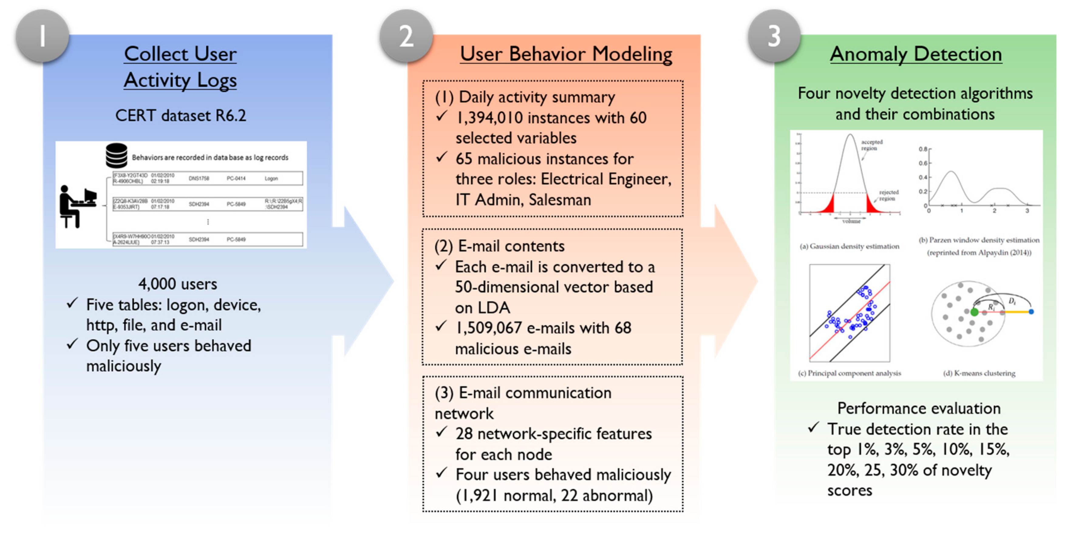
Figure 3 shows the overall framework of the insider-threat detection method developed in this study. In the user behavior-modeling phase, each user’s behaviors stored in the log system are converted to three types of datasets: daily activity summary, e-mail contents, and e-mail communication network. In the anomaly detection phase, one-class classification algorithms are trained based on the three datasets. Once a new record is available, it is input to one of these three models to predict potential malicious scores.

For the insider-threat detection domain, it is very common that a very large number of normal user activity cases is available, whereas there are only a handful or no abnormal cases available. In this case, conventional binary classification algorithms cannot be trained due to the lack of abnormal classes [19]. Alternatively, in practice, one-class classification algorithms can be used in such unbalanced data environments [29]. Unlike binary classification, one-class classification algorithms only use the normal class data to learn their common characteristics without relying on abnormal class data. Once the one-class classification model is trained, it predicts the likelihood of a newly given instance being a normal class instance. In this paper, we employed Gaussian density estimation (Gauss), Parzen window density estimation (Parzen), principal component analysis (PCA) and K-means clustering (KMC) as one-class classification algorithms for insider-threat detection, as shown in Figure 4.

Gauss [30] assumes that the entire normal user behavior cases are drawn from a single multivariate Gaussian distribution (Figure 4a), as defined in Equation (3):

$$\mathrm{p}\left(\mathrm{x}\right)=\frac{1}{{\left(2\pi \right)}^{d/2}\left|\mathsf{\Sigma }\right|}\exp \left[-\frac{1}{2}{\left(\mathrm{x}-\mathsf{\mu }\right)}^T{\mathsf{\Sigma }}^{-1}\left(\mathrm{x}-\mathsf{\mu }\right)\right]$$

(3)

Hence, training Gauss is equivalent to estimating the mean vector and covariance matrix that are most likely to generate the given dataset, as in Equations (4) and (5):

$$\mathsf{\mu }=\frac{1}{n}{\displaystyle \sum }_{{\mathrm{x}}_i\in {\mathrm{X}}_{normal}}{\mathrm{x}}_i$$

(4)

$$\mathsf{\Sigma }=\frac{1}{n-1}{\displaystyle \sum }_{{\mathrm{x}}_i\in {\mathrm{X}}_{normal}}{\left({\mathrm{x}}_i-\mathsf{\mu }\right)}^T{\mathsf{\Sigma }}^{-1}\left({\mathrm{x}}_i-\mathsf{\mu }\right)$$

(5)

where, $x_i$ is an object of a normal training instance and $X_{normal}$ is the entire learning dataset consisting of only normal instances. The anomaly score of a test observation can be determined by estimating the generation probability of the given observation with the estimated distribution parameters [31].

Parzen is one of the well-known, kernel-based, non-parametric density function estimation methods [32]. Parzen does not assume any type of prior distribution and estimates the probability density function based solely on the given observations using a kernel function K, as in Equation (6):

$$\widehat{f_h\left(x\right)}=\frac{1}{n}{\displaystyle \sum }_{i=1}^{n}K\left(\frac{x-x_i}{h}\right)$$

(6)

where, h is the bandwidth parameter of the kernel function that controls the smoothness of the estimated distribution. The kernel function (Uniform, Triangular, Gaussian, and Epanechnikov) is a non-negative function that is symmetric about the origin and has an integral value of 1 [33]. In this paper, we used the Gaussian kernel function. It is possible to estimate the density of the given dataset by adding all kernel function values for a certain location and dividing the sum by the total number of observations. If the density of a new observation is low, it is highly likely that it is abnormal.

PCA is a statistical method that finds a new set of axes that preserves the variance of the original dataset as much as possible [34]. Once these axes are determined, the high-dimensional original dataset can be mapped to a lower dimensional space without significant loss of information [15]. Solving PCA for the dataset $X\in R^{n\times p}$ is equivalent to finding the eigenvector matrix $V\in R^{n\times p}$ and the corresponding eigenvalues ${\lambda }_1,{\lambda }_2,\cdots ,{\lambda }_p$ (${\lambda }_1>{\lambda }_2>\cdots >{\lambda }_p$). Applying PCA, an instance $x\in R^p$ is mapped into a k -dimensional space (k < p) using the first k eigenvectors:

$${\mathrm{x}}^{\prime }={{\mathrm{V}}^{\prime }}^{\mathrm{T}}\mathrm{x}$$

(7)

where, $V^{\prime }\in R^{n\times k}$ consists of the first k eigenvectors. In PCA, the reconstruction error e(x), which is the difference between the original vector and its image reconstructed from the lower dimensional space to the original space, can be used as an anomaly score:

$$\mathrm{e}\left(\mathrm{x}\right)={\Vert \mathrm{x}-{{\mathrm{V}}^{\prime }{\mathrm{V}}^{\prime }}^{\mathrm{T}}\mathrm{x}\Vert }^2={\Vert \mathrm{x}\Vert }^2-{\Vert {{\mathrm{V}}^{\prime }{\mathrm{V}}^{\prime }}^{\mathrm{T}}\mathrm{x}\Vert }^2$$

(8)

KMC is a clustering method that assigns each observation ($x_j$) to the closest centroid ($c_i$) so that observations assigned to the same centroid form a cluster [15]:

$${\mathrm{argmax}}_{\mathrm{c}}{\displaystyle \sum }_{i=1}^K{\displaystyle \sum }_{x_j\in C_i}{\Vert {\mathrm{x}}_j-{\mathrm{c}}_i\Vert }^2$$

(9)

where, K is the number of clusters and is an algorithm-specific hyper-parameter that must be determined prior to executing the algorithm. We examined three K values (3, 5, and 10) in this study. Once KMC is completed based only on normal instances, the distance information between a new instance and its closest centroid is used to compute the anomaly score, as shown in Figure 4d [35]. $D_i$ is the distance between the test instance and its closest centroid while R is the radius of the cluster (the distance between the centroid and the farthest instance from the centroid in the cluster). The relative distance $D_i/R$ is the commonly used anomaly score in KMC-based anomaly detection.

In addition to the individual anomaly detection algorithms, we also consider a combination of these algorithms. Even when learning the same data, the methodology for building the optimal model for each algorithm is different, so there is no single algorithm that is superior in all situations in the machine learning field [36]. In this situation, combining different techniques can be advantageous as they generally improve the prediction performance compared to a single algorithm [36,37,38,39]. Hence, we examined all possible combinations of four individual anomaly detectors to determine the best combination for the given task and dataset. Since each algorithm has a different range of anomaly scores, we used the rank instead of score to produce the ensemble output. More specifically, for each test instance, its anomaly score ranking for each model in the ensemble is computed and the inverse of the averaged ranks was used as the anomaly score of the ensemble.

4. Results

Generally, an anomaly detection algorithm is trained based only on normal data in a situation where most instances belong to the normal class and only a few instances are from the abnormal class. Under this condition, it is impossible to set a cut-off value for detection as generally used by classification models. Hence, for daily activity-based model and e-mail contents-based model, the performances of anomaly detectors are evaluated as follows. First, the dataset is split to the training dataset, which contains 90% of randomly selected normal instances, and the test dataset, which contains the remaining 10% of normal instances and all abnormal instances. Second, an anomaly detection algorithm is trained based on the training dataset only. Third, the anomaly scores for the instances in the test dataset are computed and sorted in descending order. Finally, we compute the true detection rate using seven different cut-off values (1%, 5%, 10%, 15%, 20%, 25%, and 30%) based on Equation (10):

$$\begin{gathered} True detection rate \left(in top X\%\right) \\ = \frac{The number of malicious activities included in the top X\% anomaly scores }{Total number of malicious activities} \end{gathered}$$

(10)

In order to achieve statistically reasonable performances, we repeated the above process 30 times for each anomaly detection algorithm and used the average true detection rate in the top X% as the performance measure for insider-threat detection. Since the number of samples for e-mail network data is not as sufficient as those of daily activity data and e-main contents data, we used all normal instances for training, and anomaly scores are computed for all normal instances and abnormal instances for the e-mail network-based anomaly detection model.

4.1. Insider-Threat Detection with Daily Activity Summaries

Table 10. True detection rate of each anomaly detection algorithm based on the daily activity summary dataset (Electrical Engineer). Best performance is shown in bold and underlined (number of normal behaviors in the test set: 14,120, number of malicious behaviors in the test set: 10).

Anomaly Rank	Gauss	Parzen	PCA	KMC (K = 3)	KMC (K = 5)	KMC (K = 10)	Parzen + PCA
1%	0.5000	0.4000	0.4933	0.5233	0.5333	0.5367	0.4833
5%	0.6000	0.5000	0.6667	0.6400	0.6300	0.6333	0.7633
10%	0.6167	0.7933	0.7467	0.7033	0.6467	0.6933	0.7933
15%	0.7000	0.9000	0.7800	0.7167	0.6767	0.7333	0.8000
20%	0.7000	0.9000	0.7900	0.7500	0.6967	0.7600	0.8167
25%	0.7000	0.9000	0.8000	0.7767	0.7433	0.7767	0.8233
30%	0.7000	0.9000	0.8033	0.7767	0.7700	0.7933	0.8500

,

Table 11. True detection rate of each anomaly detection algorithm based on the daily activity summary dataset (IT Admin). Best performance is shown in bold and underlined (number of normal behaviors in the test set: 3424, number of malicious behaviors in the test set: 23).

Anomaly Rank	Gauss	Parzen	PCA	KMC (K = 3)	KMC (K = 5)	KMC (K = 10)	Parzen + PCA
1%	0.0435	0.0478	0.0739	0.0580	0.0521	0.0522	0.0971
5%	0.0435	0.1739	0.2130	0.0841	0.0739	0.0768	0.2174
10%	0.0435	0.3015	0.2304	0.1246	0.1087	0.1174	0.2580
15%	0.0971	0.3043	0.2884	0.1391	0.1275	0.1362	0.2913
20%	0.1594	0.3043	0.3348	0.2333	0.2000	0.2043	0.3246
25%	0.1739	0.3043	0.3681	0.3029	0.2681	0.2797	0.3551
30%	0.2609	0.3043	0.4087	0.3493	0.3304	0.3406	0.3928

and

Table 12. True detection rate of each anomaly detection algorithm based on the daily activity summary dataset (Salesman). Best performance is shown in bold and underlined (number of normal behaviors in the test set: 14,120, number of malicious behaviors in the test set: 32).

Anomaly Rank	Gauss	Parzen	PCA	KMC (K = 3)	KMC (K = 5)	KMC (K = 10)	Parzen + PCA
1%	0.0093	0.1177	0.0781	0.0375	0.0396	0.0281	0.1021
5%	0.0313	0.3271	0.3375	0.1083	0.0843	0.0802	0.3406
10%	0.0313	0.5677	0.5458	0.1396	0.1125	0.1135	0.6156
15%	0.6563	0.5844	0.6625	0.2604	0.1969	0.2115	0.7958
20%	0.6563	0.7781	0.7177	0.2938	0.2427	0.2416	0.8646
25%	0.6563	0.8396	0.7677	0.3240	0.2854	0.2802	0.9041
30%	0.6563	0.8719	0.8042	0.3927	0.3260	0.3219	0.9479

show the insider-threat detection performance of six individual anomaly detectors with the best combination we determined (i.e., Parzen + PCA), based on the daily activity summary dataset for the three roles: "Electrical Engineer", "IT Admin", and "Salesman". As explained in the previous section, we tested all combinations of individual models and the "Parzen + PCA” combination resulted in the best performance for 10 out of 21 cases (three roles with seven cut-off rankings) followed by "Gauss + Parzen + PCA” (5 cases). The anomaly detection performances of all possible ensemble models are provided in

Table A4. True detection rate of each anomaly detection algorithm based on the daily activity summary dataset (Electrical Engineer). Best performance is shown in bold and underlined.

Algorithm	0.10%	0.50%	1.00%	3.00%	5.00%	7.00%	10.00%
Parzen + PCA	0.3367	0.4300	0.4833	0.6833	0.7633	0.7800	0.7933
Gauss + Parzen	0.0300	0.3000	0.5767	0.7000	0.7000	0.7000	0.7000
Gauss + kMeans	0.4933	0.5000	0.5133	0.6033	0.6100	0.6300	0.6900
Gauss + PCA	0.3200	0.4667	0.5300	0.6400	0.6767	0.6867	0.6933
Parzen + kMeans	0.3133	0.3633	0.6167	0.7533	0.7633	0.7867	0.8000
kMeans + PCA	0.3400	0.5033	0.5600	0.6800	0.7267	0.7400	0.7567
Gauss + Parzen + kMeans	0.2733	0.5033	0.6033	0.7167	0.7367	0.7467	0.7900
Gauss + Parzen + PCA	0.2900	0.5133	0.6433	0.6900	0.7500	0.8000	0.8000
Gauss + kMeans + PCA	0.3267	0.5167	0.5600	0.6233	0.6867	0.7167	0.7400
Parzen + kMeans + PCA	0.3200	0.5667	0.6933	0.7533	0.7633	0.7700	0.7767
Gauss + Parzen + kMeans + PCA	0.3067	0.5567	0.6400	0.7333	0.7767	0.7967	0.8000

,

Table A5. True detection rate of each anomaly detection algorithm based on the daily activity summary dataset (IT Admin). Best performance is shown in bold and underlined.

Algorithm	0.10%	0.50%	1.00%	3.00%	5.00%	7.00%	10.00%
Parzen + PCA	0.0029	0.0710	0.0971	0.1812	0.2174	0.2232	0.2580
Gauss + Parzen	0.0130	0.0435	0.0435	0.0870	0.1275	0.1304	0.1333
Gauss + kMeans	0.0000	0.0377	0.0449	0.0710	0.0739	0.0870	0.0899
Gauss + PCA	0.0014	0.0420	0.0435	0.0478	0.1014	0.1261	0.1536
Parzen + kMeans	0.0217	0.0638	0.0797	0.1101	0.1420	0.1739	0.2043
kMeans + PCA	0.0014	0.0333	0.0739	0.1014	0.1116	0.1406	0.1971
Gauss + Parzen + kMeans	0.0275	0.0464	0.0551	0.0783	0.0971	0.1130	0.1536
Gauss + Parzen + PCA	0.0217	0.0435	0.0522	0.1101	0.1348	0.1696	0.1797
Gauss + kMeans + PCA	0.0014	0.0420	0.0565	0.0768	0.0942	0.1116	0.1565
Parzen + kMeans + PCA	0.0246	0.0246	0.0246	0.0246	0.0246	0.0246	0.0246
Gauss + Parzen + kMeans + PCA	0.0275	0.0478	0.0652	0.0928	0.1232	0.1522	0.1957

and

Table A6. True detection rate of each anomaly detection algorithm based on the daily activity summary dataset (Salesman). Best performance is shown in bold and underlined.

Algorithm	0.10%	0.50%	1.00%	3.00%	5.00%	7.00%	10.00%
Parzen + PCA	0.0344	0.0667	0.1021	0.1938	0.3406	0.4771	0.6156
Gauss + Parzen	0.0000	0.0625	0.0625	0.2188	0.3302	0.3313	0.5302
Gauss + kMeans	0.0000	0.0229	0.0510	0.0896	0.1104	0.1271	0.1583
Gauss + PCA	0.0000	0.0146	0.0635	0.2344	0.3292	0.3625	0.4125
Parzen + kMeans	0.0010	0.0167	0.0333	0.1615	0.1927	0.2615	0.3063
kMeans + PCA	0.0135	0.0354	0.0542	0.1313	0.1979	0.2323	0.2771
Gauss + Parzen + kMeans	0.0042	0.0417	0.0677	0.1854	0.2646	0.3406	0.4052
Gauss + Parzen + PCA	0.0000	0.0438	0.0688	0.2500	0.3813	0.4792	0.5750
Gauss + kMeans + PCA	0.0167	0.0438	0.0635	0.1417	0.2156	0.2677	0.3292
Parzen + kMeans + PCA	0.0000	0.0323	0.0927	0.1938	0.2646	0.3313	0.4302
Gauss + Parzen + kMeans + PCA	0.0042	0.0542	0.1010	0.2344	0.3052	0.3740	0.4813

in the Appendix A.

Table A7. The number of selected best model for each ensemble algorithm.

Number	Algorithm	The Number of Selected Best Model
1	Parzen + PCA	10
2	Gauss + Parzen	0
3	Gauss + kMeans	1
4	Gauss + PCA	0
5	Parzen + kMeans	2
6	kMeans + PCA	0
7	Gauss + Parzen + kMeans	0
8	Gauss + Parzen + PCA	5
9	Gauss + kMeans + PCA	0
10	Parzen + kMeans + PCA	3
11	Gauss + Parzen + kMeans + PCA	3

summarizes the number of best cases for each ensemble model. The proposed method exhibits effective detection performance. For example, among the top 1% of the anomaly scores predicted by Gauss for “Electrical Engineer”, half of the actual abnormal behaviors are successfully detected, which is more than 50 times higher than a random model that randomly determines 1% of test instances as anomalous behaviors.

For the “Electrical Engineer” role, when the top 1% of suspicious daily behaviors are monitored, the system can detect at most 53.66% of the actual insider threats (KMC with K = 10). It means that among the 141 test instances belonging to the 1% of highest anomaly score ranking, 5.367 out of 10 actual malicious behaviors are correctly detected, which can improve the monitoring efficiency of insider surveillance systems by prioritizing suspicious behaviors with high accuracy. This detection rate increases up to 76.33%, 79.33%, and 90% when the coverage of monitoring activities increases to the top 5%, 10%, and 15% anomaly scores, respectively. For the “IT Admin” role, detection performance is not as apparent as for “Electrical Engineer”, but it is still much better than the random guess model. The lift of the true detection rate against the random guess is 9.71 with 1% cut-off and 4.35 with 5% cut-off. For the “Salesman” role, although the detection performance is not as good as for “Electrical Engineer” with the higher cut-off values (1–15%), actual malicious activities are gradually detected when the cut-off values are lowered (15–30%). Hence, when the cut-off value is set to the top 30% of anomaly scores, 94.79% of the actual malicious behaviors are identified by the Parzen + PCA combination, which is the highest detection rate among the three roles (90% for “Electrical Engineer” and 40.87% for “IT Admin”).

Among the single algorithms, Parzen yielded the best detection rate for eight cases out of 21 cases (seven cut-off values and three roles). Although both Gauss and Parzen are based on density estimation, the assumption of Gauss, i.e., single multivariate Gaussian distribution for the entire dataset, is too strict to be applied to real datasets, which results in the worst performances in many cases. On the other hand, Parzen estimates the probability distribution in a more flexible manner, so it can be well fitted to non-Gaussian shape distributions. Note also that the Parzen + PCA combination yields the best detection performance in most cases. Compared to the detection performance of single algorithms, Parzen + PCA outperformed the single best algorithms for 10 cases. The effect of model combination is especially noticeable for the “Salesman” role.

4.2. Insider-Threat Detection with E-mail Contents

Table 13. True detection rate of each anomaly detection algorithm based on the e-mail contents dataset (Electrical Engineer). Best performance is shown in bold and underlined (number of normal behaviors in the test set: 69,405, number of malicious behaviors in the test set: 13).

Anomaly Rank	Gauss	Parzen	PCA	KMC (K = 3)	KMC (K = 5)	KMC (K = 10)	Parzen + PCA
1%	0.0000	0.0000	0.0000	0.0416	0.0458	0.0442	0.0000
5%	0.0000	0.0500	0.0016	0.1383	0.1358	0.1433	0.0008
10%	0.0750	0.0717	0.0392	0.3200	0.2717	0.2783	0.0200
15%	0.0750	0.0742	0.0417	0.4575	0.4242	0.4025	0.0500
20%	0.1016	0.0791	0.0792	0.5317	0.5133	0.4692	0.0608
25%	0.1725	0.0800	0.1592	0.6008	0.5792	0.5525	0.0808
30%	0.5608	0.0800	0.2908	0.6675	0.6542	0.6242	0.1050

,

Table 14. True detection rate of each anomaly detection algorithm based on the e-mail contents dataset (IT Admin). Best performance is shown in bold and underlined (number of normal behaviors in the test set: 17,077, number of malicious behaviors in the test set: 15).

Anomaly Rank	Gauss	Parzen	PCA	KMC (K = 3)	KMC (K = 5)	KMC (K = 10)	Parzen + PCA
1%	0.0666	0.0000	0.0600	0.0000	0.0000	0.0000	0.3756
5%	0.2022	0.3178	0.2867	0.0000	0.0000	0.0000	0.6867
10%	0.3333	0.7533	0.4178	0.0000	0.0000	0.0000	0.8333
15%	0.5156	0.8622	0.5867	0.0000	0.0000	0.0000	0.8667
20%	0.6667	0.9333	0.6867	0.0000	0.0000	0.0000	0.9044
25%	0.7378	0.9356	0.8222	0.0000	0.0000	0.0000	0.9600
30%	0.8667	0.9356	0.9067	0.0000	0.0000	0.0000	0.9867

and

Table 15. True detection rate of each anomaly detection algorithm based on the e-mail contents dataset (Salesman). Best performance is shown in bold and underlined (number of normal behaviors in the test set: 64,425, number of malicious behaviors in the test set: 40).

Anomaly Rank	Gauss	Parzen	PCA	KMC (K = 3)	KMC (K = 5)	KMC (K = 10)	Parzen + PCA
1%	0.0000	0.0000	0.0000	0.0376	0.0436	0.0487	0.0000
5%	0.0000	0.1949	0.0000	0.1154	0.1128	0.1359	0.0359
10%	0.0000	0.2359	0.0000	0.1692	0.1487	0.1385	0.1436
15%	0.0000	0.2769	0.0000	0.2154	0.2282	0.1974	0.2410
20%	0.0000	0.3026	0.0359	0.3205	0.3205	0.3128	0.2846
25%	0.0000	0.3051	0.1692	0.5180	0.5410	0.5333	0.3103
30%	0.2872	0.3103	0.4077	0.6128	0.6487	0.6564	0.3282

show the insider threat detection performance of six individual anomaly detectors with the best combination of them, i.e., Parzen + PCA, based on the e-mail contents dataset for the three roles. In contrast to the daily activity datasets, anomaly detection is more successful for “IT Admin” than the other two roles. Parzen + PCA yields a 37.56% detection rate with the top 1% of cut-off values, and it steadily increases to 98.67% for the top 30% of cut-off values. Anomaly detection performance for “Electrical Engineer” and “Salesman” are similar, the lift of the true detection rate against the random guess is above 4.5 with 1% of the cut-off value and approximately two-thirds of abnormal activities are detected with the 30% cut-off values.

Among the anomaly detection algorithms, KMC is the most effective algorithm for “Electrical Engineer” but no single algorithm yielded the best performance for “Salesman”. Another observation that is worth noting is that the performance of single anomaly detection algorithms is highly dependent on the characteristics of the dataset. Parzen + PCA yielded the highest detection rate for “IT Admin” but did not work well for “Electrical Engineers” and “Salesman”. On the other hand, KMC produced the highest detection rate for “Electrical Engineer” but it failed to detect any of the actual malicious e-mails for “IT Admin”.

4.3. Detection with E-mail Network

For the email communication history dataset among the 4000 users, four users (CDE1846, CMP2946, DNS1758, and HIS1706) sent or received numerous unusual e-mails.

Table 16. True detection rate of each anomaly detection algorithm based on the e-mail communication network dataset (CDE1846). Best performance is shown in bold and underlined (number of normal behaviors in the test set: 456, number of malicious behaviors in the test set: 9).

Anomaly Rank	Gauss	Parzen	PCA	KMC (K = 3)	KMC (K = 5)	KMC (K = 10)	Parzen + PCA
1%	0.4444	0.1111	0.1111	0.3333	0.0000	0.0000	0.1111
5%	1.0000	0.1111	0.4444	0.4444	0.0000	0.0000	0.1111
10%	1.0000	0.1111	0.5556	0.5556	0.0000	0.0000	0.4444
15%	1.0000	0.1111	0.7778	0.5556	0.0000	0.0000	0.4444
20%	1.0000	0.2222	0.7778	0.5556	0.1111	0.1111	0.5556
25%	1.0000	0.2222	0.7778	0.5556	0.1111	0.1111	0.5556
30%	1.0000	0.2222	0.7778	0.5556	0.2222	0.1111	0.6667

,

Table 17. True detection rate of each anomaly detection algorithm based on the e-mail communication network dataset (CMP2946). Best performance is shown in bold and underlined (number of normal behaviors in the test set: 474, number of malicious behaviors in the test set: 7).

Anomaly Rank	Gauss	Parzen	PCA	KMC (K = 3)	KMC (K = 5)	KMC (K = 10)	Parzen + PCA
1%	0.0000	0.0000	0.0000	0.0000	0.0000	0.0000	0.0000
5%	0.0000	0.0000	0.0000	0.0000	0.0000	0.0000	0.0000
10%	0.0000	0.0000	0.0000	0.0000	0.0000	0.0000	0.0000
15%	0.0000	0.0000	0.0000	0.0000	0.0000	0.0000	0.0000
20%	0.3333	0.0000	0.3333	0.0000	0.0000	0.0000	0.0000
25%	0.6667	0.0000	1.0000	0.0000	0.0000	0.0000	0.3333
30%	0.6667	0.0000	1.0000	0.0000	0.0000	0.0000	0.3333

,

Table 18. True detection rate of each anomaly detection algorithm based on the e-mail communication network dataset (DNS1758). Best performance is shown in bold and underlined (number of normal behaviors in the test set: 498, number of malicious behaviors in the test set: 3).

Anomaly Rank	Gauss	Parzen	PCA	KMC (K = 3)	KMC (K = 5)	KMC (K = 10)	Parzen + PCA
1%	0.0000	0.0000	0.0000	0.3333	0.3333	0.3333	0.0000
5%	0.3333	0.0000	0.0000	0.6667	0.6667	0.3333	0.0000
10%	0.3333	0.0000	0.3333	1.0000	1.0000	0.3333	0.0000
15%	0.6667	0.3333	0.6667	1.0000	1.0000	0.3333	0.0000
20%	0.6667	0.3333	0.6667	1.0000	1.0000	0.3333	0.3333
25%	0.6667	0.3333	0.6667	1.0000	1.0000	0.3333	0.3333
30%	0.6667	0.3333	0.6667	1.0000	1.0000	0.6667	0.3333

and

Table 19. True detection rate of each anomaly detection algorithm based on the e-mail communication network dataset (HIS1706). Best performance is shown in bold and underlined (number of normal behaviors in the test set: 493, number of malicious behaviors in the test set: 3).

Anomaly Rank	Gauss	Parzen	PCA	KMC (K = 3)	KMC (K = 5)	KMC (K = 10)	Parzen + PCA
1%	0.0000	0.0000	0.0000	0.3333	0.3333	0.3333	0.0000
5%	0.3333	0.0000	0.0000	0.6667	0.6667	0.3333	0.0000
10%	0.3333	0.0000	0.3333	1.0000	1.0000	0.3333	0.0000
15%	0.6667	0.3333	0.6667	1.0000	1.0000	0.3333	0.0000
20%	0.6667	0.3333	0.6667	1.0000	1.0000	0.3333	0.3333
25%	0.6667	0.3333	0.6667	1.0000	1.0000	0.3333	0.3333
30%	0.6667	0.3333	0.6667	1.0000	1.0000	0.6667	0.3333

show the user-level insider-threat detection performance of the anomaly detection models based on the e-mail communication network dataset.

It is worth noting that all the malicious e-mail communication of three users (CDE1846, DNS1758, and HIS1706) were successfully detected by the anomaly detection algorithms using at most 25% of the cut-off value. Surprisingly, Gauss yielded a 100% detection rate by monitoring only the top 5% of suspicious instances for user CDE1846, whereas KMC succeeded in detecting all the malicious instances of user HIS1706 by monitoring the top 10% of suspicious instances. The only exceptional user is CMP2946, for whom the anomaly detection model failed to detect more than 30% of actual malicious e-mail communications although the cut-off value was lowered to the top 30% of anomaly scores. Another interesting observation is that unlike the other two datasets, model combinations did not achieve a better detection performance than individual models. The best algorithms for each user are Gauss for CDE1846 and KMC for HIS1706. For the other two users, none of the single algorithms yielded the highest detection rate for all cut-off values.

5. Conclusions

In this paper, we proposed an insider-threat detection framework based on user behavior modeling and anomaly detection algorithms. During the user behavior modeling, individual users’ heterogeneous behaviors are transformed into a structured dataset where each row is associated with an instance (user-day, e-mail content, user-week) and each column is associated with input variables for anomaly detection models. Based on the CERT dataset, we constructed three datasets, i.e., daily activity summary dataset based on user activity logs, an e-mail content dataset based on topic modeling, and an e-mail communication network dataset based on the user’s account and sending/receiving information. Based on these three datasets, we constructed insider-threat detection models by employing machine learning-based anomaly detection algorithms to simulate real-word organizations in which only a few insiders’ behaviors are actually potentially malicious.

Experimental results show that the proposed framework can work reasonably well to detect insiders’ malicious behaviors. Based on the daily activity summary dataset, the anomaly detection model yielded at most 53.67% of the detection rate by only monitoring the top 1% of suspicious instances. When the monitoring coverage was extended to the top 30% of anomaly scores, more than 90% of actual abnormal behaviors were detected for two roles among the three evaluated. Based on the e-mail content datasets, at most 37.56% of malicious e-mails were detected with the 1% cut-off value while the detection rate increased to 65.64% (98.67% at most) when the top 30% of suspicious e-mails were monitored. Based on the e-mail communication network dataset, all the malicious instances were correctly identified for three out of four tested users.

Although the proposed framework was empirically verified, there are some limitations in the current research, which led us to future research directions. First, we constructed three structured datasets to train the anomaly detection algorithms. Because the instances of these three datasets are different from each other (a user’s daily activity, an e-mail’s topic distribution, a user’s weekly e-mail communication), anomaly detection models are independently trained based on each dataset. If these different anomaly detection results are properly integrated, it may be possible to achieve a better insider-threat detection performance. Second, we built the insider-threat detection model based on specific time unit, e.g., a day. In order words, this approach can detect malicious behaviors based on the batch process, but cannot detect them in a real-time. Hence, it could be worth developing a sequence-based insider-threat detection model that can process online stream data. Third, the proposed model is purely data-driven. However, in the security domain, combining the knowledge of experts and a pure data-driven machine learning model can enhance the insider-threat detection performance. Lastly, although the CERT dataset was carefully constructed containing various threat scenarios designed by domain experts, it is still a simulated and artificially generated dataset. If the proposed framework can be verified through a real-world dataset, its practical applicability could be more validated.

References

- Lindauer, B.; Glasser, J.; Rosen, M.; Wallnau, K. Generating Test Data for Insider Threat Detectors. JoWUA 2014, 5, 80–94. [Google Scholar]
- Schultz, E.E. A framework for understanding and predicting insider attacks. Comput. Secur. 2012, 21, 526–531. [Google Scholar] [CrossRef]
- Legg, P.A. Visualizing the insider threat: Challenges and tools for identifying malicious user activity. In Proceedings of the 2015 IEEE Symposium on Visualization for Cyber Security (VizSec), Chicago, IL, USA, 25 October 2015; pp. 1–7. [Google Scholar]
- Ted, E.; Goldberg, H.G.; Memory, A.; Young, W.T.; Rees, B.; Pierce, R.; Huang, D.; Reardon, M.; Bader, D.A.; Chow, E. Detecting insider threats in a real corporate database of computer usage activity. In Proceedings of the 19th ACM SIGKDD International Conference on Knowledge Discovery and Data Mining, Chicago, IL, USA, 11–14 August 2013; pp. 1393–1401. [Google Scholar]
- Mather, T.; Kumaraswamy, S.; Latif, S. Cloud Security and Privacy: An Enterprise Perspective on Risks and Compliance; O’Reilly Media, Inc.: Newton, MA, USA, 2009. [Google Scholar]
- Salem, M.B.; Hershkop, S.; Stolfo, S.J. A survey of insider attack detection research. Insid. Attack Cyber Secur. 2008, 39, 69–90. [Google Scholar]
- Theoharidou, M.; Kokolakis, S.; Karyda, M.; Kiountouzis, E. The insider threat to information systems and the effectiveness of ISO17799. Comput. Secur. 2005, 24, 472–484. [Google Scholar] [CrossRef]
- Wong, W.-K.; Moore, A.; Cooper, G.; Wagner, M. Rule-based anomaly pattern detection for detecting disease. In Proceedings of the Eighteenth National Conference on Artificial Intelligence (AAAI-02), Edmonton, AB, Canada, 28 July–1 August 2002; pp. 217–223. [Google Scholar]
- Cappelli, D.M.; Moore, A.P.; Trzeciak, R.F. The CERT Guide to Insider Threats: How to Prevent, Detect, and Respond to Information Technology Crimes (Theft, Sabotage, Fraud); Addison-Wesley: Boston, MA, USA, 2012. [Google Scholar]
- Eldardiry, H.; Sricharan, K.; Liu, J.; Hanley, J.; Price, B.; Brdiczka, O.; Bart, E. Multi-source fusion for anomaly detection: Using across-domain and across-time peer-group consistency checks. JoWUA 2014, 5, 39–58. [Google Scholar]
- Lunt, T.F.; Jagannathan, R.; Lee, R.; Whitehurst, A.; Listgarten, S. Knowledge-based intrusion detection. In Proceedings of the Annual AI Systems in Government Conference, Washington, DC, USA, 27–31 March 1989; pp. 102–107. [Google Scholar]
- Eberle, W.; Graves, J.; Holder, L. Insider threat detection using a graph-based approach. J. Appl. Secur. Res. 2010, 6, 32–81. [Google Scholar] [CrossRef]
- Parveen, P.; Evans, J.; Thuraisingham, B.; Hamlen, K.W.; Khan, L. Insider threat detection using stream mining and graph mining. In Proceedings of the Privacy, Security, Risk and Trust (PASSAT) and 2011 IEEE Third Inernational Conference on Social Computing (SocialCom), Boston, MA, USA, 9–11 October 2011; pp. 1102–1110. [Google Scholar]
- Mayhew, M.; Atighetchi, M.; Adler, A.; Greenstadt, R. Use of machine learning in big data analytics for insider threat detection. In Proceedings of the MILCOM 2015—2015 IEEE Military Communications Conference, Tampa, FL, USA, 26–28 October 2015; pp. 915–922. [Google Scholar]
- Alpaydin, E. Introduction to Machine Learning; MIT Press: Cambridge, MA, USA, 2014. [Google Scholar]
- Gavai, G.; Sricharan, K.; Gunning, D.; Hanley, J.; Singhal, M.; Rolleston, R. Supervised and Unsupervised methods to detect Insider Threat from Enterprise Social and Online Activity Data. JoWUA 2015, 6, 47–63. [Google Scholar]
- Ho, T.K. Random decision forests. In Proceedings of the 3rd International Conference on Document Analysis and Recognition, Montreal, QC, Canada, 14–16 August 1995; pp. 278–282. [Google Scholar]
- Liu, F.T.; Ting, K.M.; Zhou, Z.-H. Isolation forest. In Proceedings of the 2008 Eighth IEEE International Conference on Data Mining, Pisa, Italy, 15–19 December 2008; pp. 413–422. [Google Scholar]
- Sun, Y.; Wong, A.K.; Kamel, M.S. Classification of imbalanced data: A review. Int. J. Pattern Recognit. Artif. Intell. 2009, 23, 687–719. [Google Scholar] [CrossRef]
- Glasser, J.; Lindauer, B. Bridging the gap: A pragmatic approach to generating insider threat data. In Proceedings of the 2013 IEEE Security and Privacy Workshops, San Francisco, CA, USA, 23–24 May 2013; pp. 98–104. [Google Scholar]
- McGough, A.S.; Arief, B.; Gamble, C.; Wall, D.; Brennan, J.; Fitzgerald, J.; van Moorsel, A.; Alwis, S.; Theodoropoulos, G.; Ruck-Keene, E. Detecting insider threats using Ben-ware: Beneficial intelligent software for identifying anomalous human behavior. J. Wirel. Mob. Netw. Ubiquitous Comput. Dependable Appl. 2015, 6, 1–44. [Google Scholar]
- Young, W.T.; Goldberg, H.G.; Memory, A.; Sartain, J.F.; Senator, T.E. Use of domain knowledge to detect insider threats in computer activities. In Proceedings of the 2013 IEEE Security and Privacy Workshops, San Francisco, CA, USA, 23–24 May 2013; pp. 60–67. [Google Scholar]
- Nellikar, S. Insider Threat Simulation and Performance Analysis of Insider Detection Algorithms with Role Based Models. Master’s Thesis, University of Illinois at Urbana-Champaign, Champaign County, IL, USA, 19 May 2010. [Google Scholar]
- Guyon, I.; Elisseeff, A. An introduction to variable and feature selection. J. Mach. Learn. Res. 2003, 3, 1157–1182. [Google Scholar]
- Blei, D.M.; Ng, A.Y.; Jordan, M.I. Latent dirichlet allocation. J. Mach. Learn. Res. 2003, 3, 993–1022. [Google Scholar]
- Wallach, H.M. Topic modeling: Beyond bag-of-words. In Proceedings of the 23rd International Conference on Machine Learning, Pittsburgh, PA, USA, 25–29 June 2006; ACM: New York, NY, USA; pp. 977–984. [Google Scholar]
- Levandowsky, M.; Winter, D. Distance between sets. Nature 1971, 234, 34–35. [Google Scholar] [CrossRef]
- Wasserman, S.; Faust, K. Social Network Analysis: Methods and Analysis; Cambridge University Press: Cambridge, UK, 1994. [Google Scholar]
- Ali, A.; Shamsuddin, S.M.; Ralescu, A.L. Classification with class imbalance problem. Int. J. Adv. Soft Comput. Appl. 2013, 5, 1–38. [Google Scholar]
- Chandola, V.; Banerjee, A.; Kumar, V. Anomaly detection: A survey. ACM Comput. Surv. 2009, 41, 1–58. [Google Scholar] [CrossRef]
- Barnett, V.; Lewis, T. Outliers in Statistical Data; Wiley: New York, NY, USA, 1994. [Google Scholar]
- Duda, R.O.; Hart, P.E.; Stork, D.G. Pattern Classification; John Wiley & Sons: Hoboken, NJ, USA, 2012. [Google Scholar]
- Muller, K.-R.; Mika, S.; Ratsch, G.; Tsuda, K.; Scholkopf, B. An introduction to kernel-based learning algorithms. IEEE Trans. Neural Netw. 2001, 12, 181–201. [Google Scholar] [CrossRef] [PubMed]
- Wold, S.; Esbensen, K.; Geladi, P. Principal component analysis. Chemom. Intell. Lab. Syst. 1987, 2, 37–52. [Google Scholar] [CrossRef]
- Markou, M.; Singh, S. Novelty detection: A review—Part 1: Statistical approaches. Signal Process. 2003, 83, 2481–2497. [Google Scholar] [CrossRef]
- Fernández-Delgado, M.; Cernadas, E.; Barro, S.; Amorim, D. Do we need hundreds of classifiers to solve real world classification problems. J. Mach. Learn. Res. 2014, 15, 3133–3181. [Google Scholar]
- Woźniak, M.; Graña, M.; Corchado, E. A survey of multiple classifier systems as hybrid systems. Inf. Fusion 2014, 16, 3–17. [Google Scholar] [CrossRef]
- Britto, A.S.; Sabourin, R.; Oliveira, L.E. Dynamic selection of classifiers—A comprehensive review. Pattern Recognit. 2014, 47, 3665–3680. [Google Scholar] [CrossRef]
- Tang, E.K.; Suganthan, P.N.; Yao, X. An analysis of diversity measures. Mach. Learn. 2006, 65, 247–271. [Google Scholar] [CrossRef] [Green Version]
Figure 1.
Latent Dirichlet allocation (LDA) process and its two outputs. (a) LDA document generation process, (b)An illustrative example of the LDA document generation process, (c) Two outputs of LDA ((c-1) Per-document topic proportions (), (c-2) Per-topic word distributions ()).
Figure 2.
Example of email communication network.
Figure 3.
Insider-threat detection framework.
Figure 4.
Four anomaly detection algorithms used in this paper. (a) Gaussian density estimation, (b) Parzen window density estimation (reprinted from Alpaydin (2014)), (c) Principal component analysis (PCA), and (d) K-means clustering (KMC).